Article

Super-Resolution Range and Velocity Estimations for SFA-OFDM Radar

1
Department of Remote Sensing Science and Technology, Xidian University, Xi’an 710071, China
2
National Laboratory of Radar Signal Processing, Xidian University, Xi’an 710071, China
3
Academy of Advanced Interdisciplinary Research, Xidian University, Xi’an 710071, China
*
Author to whom correspondence should be addressed.
Remote Sens. 2022, 14(2), 278; https://doi.org/10.3390/rs14020278
Submission received: 14 December 2021 / Revised: 3 January 2022 / Accepted: 6 January 2022 / Published: 7 January 2022

Abstract

:
Sparse frequency agile orthogonal frequency division multiplexing (SFA-OFDM) signal brings excellent performance to electronic counter-countermeasures (ECCM) and reduces the complexity of the radar system. However, frequency agility makes coherent processing a much more challenging task for the radar, which leads to the discontinuity of the echo phase in a coherent processing interval (CPI), so the fast Fourier transform (FFT)-based method is no longer a valid way to complete the coherent integration. To overcome this problem, we proposed a novel scheme to estimate both super-resolution range and velocity. The subcarriers of each pulse are firstly synthesized in time domain. Then, the range and velocity estimations for the SFA-OFDM radar are regarded as the parameter estimations of a linear array. Finally, both the super-resolution range and velocity are obtained by exploiting the multiple signal classification (MUSIC) algorithm. Simulation results are provided to demonstrate the effectiveness of the proposed method.

1. Introduction

With the rapid development of electronic technology, orthogonal frequency division multiplexing (OFDM) technology has already been widely applied in communication systems [1,2,3]. Its advantages include robustness against Inter Symbol Interference (ISI) and Inter Carrier Interference (ICI), high spectral efficiency and ease of implementation [4,5], etc.
In recent years, OFDM has also attracted more and more attention in radar applications, such as radar imaging [6,7], radar detection [8,9] and integration radar and communication [10,11,12]. As a multi-carrier wide-band radar, the OFDM radar has the major drawback of a large baseband bandwidth. Meanwhile, to improve the range resolution, a larger bandwidth is also necessary. This requires that OFDM radar hardware has sufficient high sampling and data processing rates. To reduce the hardware requirements, many researchers are studying the stepped-OFDM radar, the core idea of which is to reduce the instantaneous bandwidth of the OFDM radar. In [13], an OFDM phase-coded stepped-frequency (OFDM-PCSF) waveform is presented, whereby a high range resolution (HRR) is achieved by synthesizing multiple narrowband signals. However, this only applies to low velocity targets. A similar stepped-carrier OFDM-radar waveform is investigated in [14], which can simultaneously achieve the high-resolution range and velocity but with a much lower baseband bandwidth. Nuss et al. [15,16] propose a frequency comb OFDM radar signal to overcome the hardware limitations. It also can obtain HRR profiles, but its unambiguous velocity is sustained at the cost of a decreased unambiguous range.
Furthermore, frequency agility [17,18,19] is introduced into the OFDM radar by Lellouch et al. [20,21]. Each pulse transmits a narrowband signal, while the carrier frequencies are randomly varied from pulse to pulse, bringing not only excellent performance in electronic counter-countermeasures (ECCM), but also significantly reducing the instantaneous bandwidth of the OFDM radar system [22]. However, frequency agility leads to the discontinuity of echo phase in a coherent processing interval (CPI), so the fast Fourier transform (FFT)-based method cannot complete coherent integration. In [20], different patterns for frequency agility based on OFDM waveform are investigated. It shows that the spread subcarriers hopping presents a very sharp peak in both delay and scale domains. Meanwhile, the Doppler processing concept is proposed. Subcarriers with the same frequencies are utilized to process Doppler, and the rest contribute to agility. Nevertheless, this method requires a longer coherent processing time, and range cell migration (RCM) may be needed. It cannot obtain super-resolution range and velocity simultaneously. A similar frequency agile stepped waveform is proposed [21]. The multiple narrowband signals are synthesized to obtain the HRR profile, which is only suitable for a single stationary or low-speed point target. In [23], a frequency-agile sparse OFDM radar with short sequences of narrowband pulses of different bandwidths is proposed, and the compressed sensing (CS) theory is applied to obtain a high-resolution range-velocity profile. In [24], the influence of a state-of-the-art frequency-modulated continuous wave (FMCW) on stepped and sparse OFDM is examined, and zeroing of interfered samples in the frequency domain is used to suppress FMCW-interference. An interference-robust processing for OFDM radar signals using CS is presented in [25]. This method is not only suitable for random OFDM, but also applied for stepped or standard OFDM.
Based on the previous work, the super-resolution range and velocity estimations for the sparse frequency agile OFDM (SFA-OFDM) radar is studied in this paper. Similarly to the frequency agile stepped OFDM waveform proposed in [20,23], the SFA-OFDM radar signal’s agile pattern is grouped subcarrier frequency random hopping, and the bandwidth of each pulse is equal. However, the difference is that each SFA-OFDM radar subcarrier is a narrow-band linear frequency modulation (LFM) signal, and some frequencies are unused during a CPI, i.e., the number of pulses in a CPI is less than the total number of available frequencies. The SFA-OFDM radar signal is sparse [26] in the time–frequency domain. Therefore, it is difficult to track and predict by jamming.
The main works in our paper are as follows. Firstly, for a moving target, the SFA-OFDM radar’s mathematical model is derived. A merit of the SFA-OFDM radar is that the ECCM performance is more robust and the limitations of system hardware are overcome. Secondly, to obtain the super-resolution range–velocity of the SFA-OFDM radar simultaneously, we introduce a signal processing method, in which the parameter estimations of the SFA-OFDM radar is equivalent to that of a linear array, and the MUSIC algorithm [27] is applied to achieve the super-resolution range and velocity estimations. Thirdly, the performance of the proposed parameter estimations algorithm for the SFA-OFDM radar is analyzed. The Cramér-Rao lower bounds (CRLBs) on parameter estimations using the SFA-OFDM radar signal are derived. Finally, the effectiveness of the proposed method is proved by several simulation experiments. Compared with the Doppler processing method proposed in [20], the proposed method solves the conflict between the frequency agility and coherent processing. It can obtain the super-resolution range and velocity in a CPI. Its range–velocity resolution is only related to the size of the grid, and the smaller the grid size, the higher the resolution will be.
The remainder of this paper is organized as follows. In Section 2, the mathematical model of the SFA-OFDM radar signal is established. Section 3 describes the proposed range–velocity estimation scheme. The performance of the proposed method is discussed in Section 4. Several numerical simulation experiments are presented to validate the proposed method in Section 5. Finally, Section 6 concludes the paper.

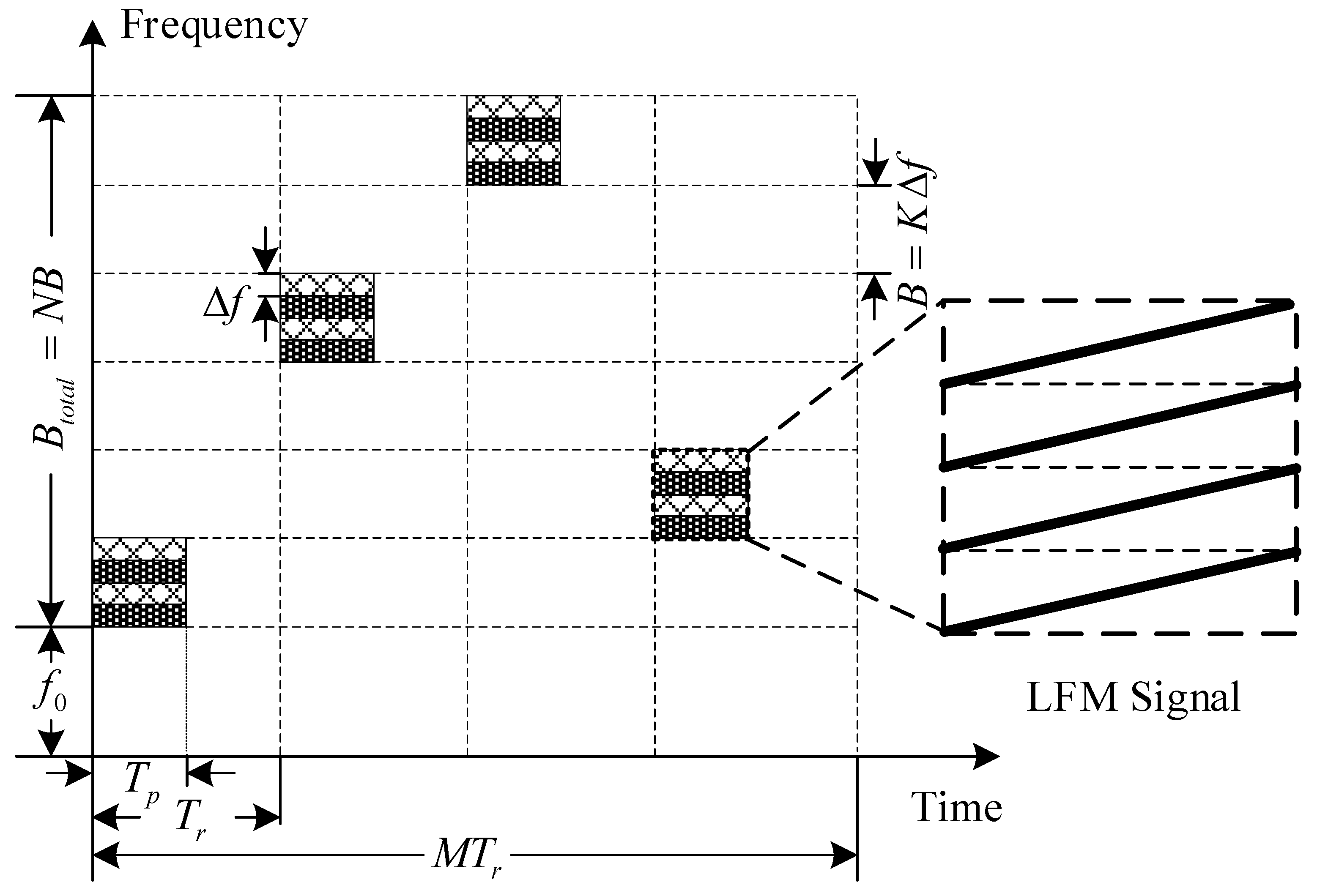
2. SFA-OFDM Radar Signal Model

In this section, first, the SFA-OFDM radar signal is introduced. Then, the received signal model for the moving target is established.
An illustration of the SFA-OFDM radar signal model [20,28] is given in Figure 1. We assume that the SFA-OFDM radar transmits M pulses in a CPI. Each pulse consists of K orthogonal subcarriers with bandwidth Δ f , and all the subcarriers are the narrow-band LFM signal. The initial carrier frequency of m th pulse is f m = f 0 + a m B , m { 0 , 1 , , M 1 } , where f 0 denotes the lowest carrier frequency, a m is the m th frequency modulation code which is randomly selected from N, a m { 0 , 1 , , N 1 } , N is the total number of available frequencies, and N > M . B is the frequency step. The radio frequency (RF) signal of the SFA-OFDM radar can be modeled as
s t ( t ) = m = 0 M 1 s b ( t ) · exp ( j 2 π f m t ) = m = 0 M 1 k = 0 K 1 ω k rect ( t m T r T p ) · exp [ j π γ ( t m T r ) 2 ] · exp [ j 2 π ( f m + k Δ f ) t ] ,
where ω k represents the frequency weighting coefficient of the k th subcarrier. T r and γ are, respectively, the pulse repetition interval and the chirp rate. T p denotes the pulse duration and rect ( · ) is the standard rectangle function.
rect ( x ) = { 1 , 0 x 1 , 0 , o t h e r w i s e .
Assume that there is a target which is an isotropic point scatterer model in a scenario, and it is moving along the line of sight of the radar with a uniform speed. The radial range and velocity are, respectively, r 0 and v. Received radar echo is a delay of the transmitted signal. At time t m , the range between the radar and target is r ( t m ) = r 0 + v t m . Then, the delay of the m th pulse can be written as
τ ( t m ) = 2 r ( t m ) c = 2 ( r 0 + v t m ) c ,
where t m = m T r stands for the slow time and c is the speed of light. The radar echo can be described as
s r ( t ) = m = 0 M 1 k = 0 K 1 ξ ω k rect [ t m T r τ ( t m ) T p ] · exp { j π γ [ t m T r τ ( t m ) ] 2 } · exp { j 2 π ( f m + k Δ f ) [ t τ ( t m ) ] } + η ( t ) ,
where ξ denotes the back scattering coefficient of the target and η ( t ) is additive white Gaussian noise with zero mean. The SFA-OFDM radar carrier frequencies are randomly varied from pulse to pulse. Hence, the received echo from the m th pulse needs to multiply by the expression exp [ j 2 π ( f m + k Δ f ) t ] . After down-conversion, the received signal can be formulated as
s r ( t ) = m = 0 M 1 k = 0 K 1 σ ω k rect [ t m T r τ ( t m ) T p ] · exp { j π γ [ t m T r τ ( t m ) ] 2 } · exp [ j 2 π f m τ ( t m ) ] · exp [ j 2 π k Δ f τ ( t m ) ] + η ( t ) · exp [ j 2 π ( f m + k Δ f ) t ] .

3. Signal Processing

In this section, we propose a new scheme to estimate the range and velocity for the SFA-OFDM radar. First, the subcarriers of each pulse are synthesized to obtain an LFM signal with a larger bandwidth. Then, the pulse compression is performed in each pulse. Finally, the MUSIC algorithm is applied to estimate the super-resolution range and velocity.

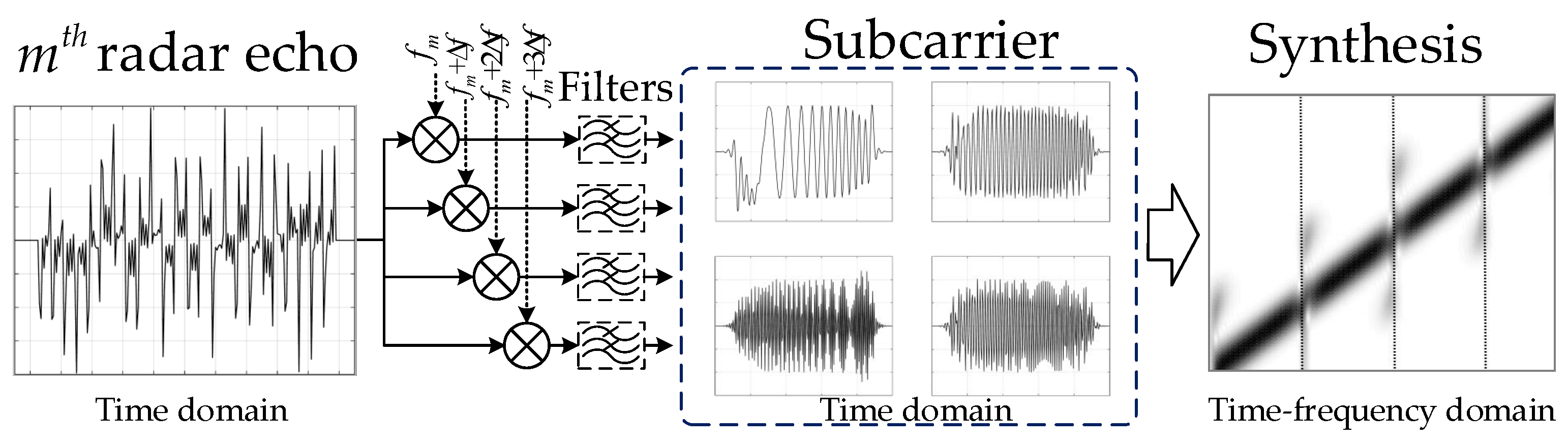
3.1. Subcarrier Synthesis Processing

As shown in Figure 2, after down-conversion, the low-pass filter banks are utilized to separate the subcarriers. The pass band of each filter is equivalent to the bandwidth of the subcarrier, i.e., the pass band of each filter is [ 0 , Δ f ] . Let η ( t ) = η ( t ) · exp [ j 2 π ( f m + k Δ f ) t ] . After filtering, the k th subcarrier of the m th pulse can be represented as
s m , k ( t ) = ξ ω k rect [ t m T r τ ( t m ) T p ] · exp { j π γ [ t m T r τ ( t m ) ] 2 } · exp [ j 2 π f m τ ( t m ) ] · exp [ j 2 π k Δ f τ ( t m ) ] + η m , k ( t ) ,
substituting (3) into (6), we can further obtain
s m , k ( t ) = ξ ω k rect [ t m T r τ ( t m ) T p ] · exp { j π γ [ t m T r τ ( t m ) ] 2 } · exp [ j 4 π ( f m + k Δ f ) r 0 c ] · exp [ j 4 π ( f m + k Δ f ) v t m c ] + η m , k ( t ) .
Next, we synthesize the K subcarrier in time domain. First, the time shift is performed on the subcarrier. Because the time shift interval is usually a non-integer multiple of the sampling interval, we transform the signal from the time domain to the frequency domain to realize the time shift. The k th time-shift phase factor is [29]
ϕ k t i m e = exp [ j 2 π T p f r ( k + 1 K 2 ) ]
where f r { f s 2 , f s 2 } , f s is the sampling rate. After the time shift, the k th subcarrier of the m th pulse is as follows
s m , k ( t ^ ) = IFFT { ϕ k t i m e FFT [ s m , k ( t ) ] } = ξ ω k rect [ t ^ τ ( t m ) T p ( k + 1 / 2 K / 2 ) T p ] · exp { j π γ [ t ^ τ ( t m ) T p ( k + 1 / 2 K / 2 ) ] 2 } · exp [ j 4 π ( f m + k Δ f ) r 0 c ] · exp [ j 4 π ( f m + k Δ f ) v t m c ] + η m , k ( t ) ,
where t ^ = t m T r is the fast time. Then, the frequency shift is needed to reconstruct the signal spectrum. Like the time shift, the frequency shift is realized by multiplying the frequency-shift phase factor in time domain, and the k th frequency-shift phase factor can be described as [29]
ϕ k f r e = exp [ j 2 π Δ f t ^ ( k + 1 K 2 ) ] ,
after the frequency shift, the k th subcarrier of the m th pulse can be represented as
s m , k ( t ^ ) = s m , k ( t ) · ϕ k f r e = ξ ω k rect [ t ^ τ ( t m ) T p ( k + 1 / 2 K / 2 ) T p ] · exp { j π γ [ t ^ τ ( t m ) ] 2 } · exp [ j 4 π f m ( r 0 c ) ] · exp [ j 4 π f m ( v t m c ) ] · exp { j π γ [ T p ( k + 1 K 2 ) ] 2 } + η m , k ( t ) ,
where f m = f m ( 1 K 2 ) Δ f . In (11), there is a phase factor exp { j π γ [ T p ( k + 1 K 2 ) ] 2 } that may result in the signal phase discontinuity after subcarrier synthesis processing. Hence, the subcarrier phase should be corrected. The k th phase correction factor is [29]
ϕ k c o r r = exp { j π γ [ T p ( k + 1 K 2 ) ] 2 } ,
then, the k th subcarrier can be expressed as
s m , k ( t ^ ) = ξ ω k rect [ t ^ τ ( t m ) T p ( k + 1 / 2 K / 2 ) T p ] · exp { j π γ [ t ^ τ ( t m ) ] 2 } · exp [ j 4 π f m ( r 0 c ) ] · exp [ j 4 π f m ( v t m c ) ] + η m , k ( t ) ,
to simplify the analysis, let ω k = 1 . To acquire a wideband LFM signal, the K subcarriers should be superimposed in time domain, and the m th wideband LFM signal can be written as
S m ( t ^ ) = k = 0 K s m , k ( t ^ ) = k = 0 K ξ rect [ t ^ τ ( t m ) T p ( k + 1 / 2 K / 2 ) T p ] · exp { j π γ [ t ^ τ ( t m ) ] 2 } · exp [ j 4 π f m ( r 0 c ) ] · exp [ j 4 π f m ( v t m c ) ] + η m ( t ) .
From (14), we can see that the subcarriers of m th pulse are synthesized to produce an LFM signal with bandwidth K Δ f . The carrier frequency of each pulse is f m that is randomly hopping from pulse to pulse. Thus, the SFA-OFDM radar can be equivalent to the traditional frequency agile radar, i.e., each pulse is an LFM signal and the carrier frequencies are varied in a random manner [30].
After the pulse compression, the m th pulse can be expressed as
S m ( t ^ ) = S m ( t ^ ) S ˜ ( t ^ ) = ξ sinc { π B [ t ^ τ ( t m ) ] } · exp { j π γ [ t ^ τ ( t m ) ] 2 } · exp { j 4 π [ f 0 ( 1 K ) 2 Δ f ] ( r 0 c ) } · exp [ j 4 π a m B ( r 0 c ) ] · exp [ j 4 π f m ( v t m c ) ] + η m ( t ^ ) ,
where S ˜ ( t ^ ) = rect ( t ^ K T p ) · exp [ j π γ ( t ^ ) 2 ] , ⊗ denotes convolution operation, ξ = ξ · δ , and δ is the range compression gain.

3.2. Super-Resolution Range and Velocity Estimations

In order to facilitate the analysis, Formulae (15) can be rewritten as
S m ( t ^ ) = A ( t ^ ) · φ r ( m ) · φ v ( m ) + η m ( t ) ,
where A ( t ^ ) = ξ sinc { π B [ t ^ τ ( t m ) ] } · exp { j π γ [ t ^ τ ( t m ) ] 2 } · exp { j 4 π [ f 0 ( 1 K ) 2 Δ f ] ( r 0 c ) } is the constant terms. φ r ( m ) = exp [ j 4 π a m B ( r 0 c ) ] and φ v ( m ) = exp [ j 4 π f m ( v t m c ) ] denote the range phase term and the velocity term, respectively. Formulae (16) is the single pulse echo signal. In radar system, we need to deal with echo data in a CPI. Therefore, we rearrange the M pulses into a data matrix along the slow time. The data matrix can be represented as
S = a ( r ) a ( v ) · A + η ,
where ⊙ stands for Hadamard product. S = [ S 0 ( t ^ ) , S 1 ( t ^ ) , , S M 1 ( t ^ ) ] T , a ( r ) = [ φ r ( 0 ) , φ r ( 1 ) , , φ r ( M 1 ) ] T , a ( v ) = [ φ v ( 0 ) , φ v ( 1 ) , , φ v ( M 1 ) ] T and η = [ η 0 ( t ^ ) , η 1 ( t ^ ) , η M 1 ( t ^ ) ] T . [ · ] T represents the transpose operator. Furthermore, let a ( r , v ) = a ( r ) a ( v ) that contains the range and velocity information of the target, and all the received signals can be rewritten as
S = a ( r , v ) A + η .
From (18), we can see that the received signal model of the SFA-OFDM radar is similar to that of the linear array. The data matrix S can be equivalent to the multiple synchronous sampling of the linear array [31] with M array elements. The number of sampling points of the SFA-OFDM radar along the fast time is similar to the number of snapshots of the linear array. The vector a ( r , v ) is equivalent to the array steering vector. Consequently, the range and velocity estimations for the SFA-OFDM radar can be regarded as the two-dimensional parameter estimations of the array signal.
In array signal processing, the MUSIC algorithm can be applied to obtain the super-resolution parameter estimation. Similarly, in this paper, we use the MUSIC algorithm to estimate the range and velocity for the SFA-OFDM radar. The steps are as follows, the covariance matrix of the echo data is used to acquire the signal and noise subspace based on eigenvalue decomposition at first. Then, the spectral function is constructed using the orthogonality between signal and noise subspace. Finally, the range and velocity of the target are estimated by spectral peak search.
From (18), we can obtain the covariance matrix of the echo data. The covariance matrix of the echo data is
R S = E { S ( S ) H } = a ( r , v ) E { A A H } a ( r , v ) H + σ 2 I ,
where E { · } denotes the expectation operator and ( · ) H represents the complex conjugate transpose operator. The eigenvalue decomposition of the covariance matrix R S can be described as
R S = U S Λ S U S H ,
where U S = [ u 0 , u 1 , , u M 1 ] is an eigenvector matrix. Λ S is a diagonal matrix that consists of the eigenvalues of R S . For the MUSIC algorithm, the number of targets should be estimated in advance when we acquire signal and noise subspace. In this paper, we assume that the number of targets is known. Equation (20) can be rewritten as
R S = U s Λ s U s H + U n Λ n U n H ,
where U s denotes the signal subspace. Λ s is a diagonal matrix with elements being the eigenvalue of signal subspace. U n represents the noise subspace. Λ n is a diagonal matrix with elements being the eigenvalue of noise subspace.
To obtain the range and velocity, we need to search over all the possible range and velocity of the target. Hence, we usually divide the range–velocity space uniformly into multiple grids. The size of the grid is related to the range and velocity resolution, i.e., the smaller the grid is, the higher the range and velocity resolution will be. In this paper, we divide the unambiguous range and velocity into X × Y grids uniformly. The search matrix can be written as
A ˜ = [ a ( r 0 , v 0 ) , a ( r 0 , v 2 ) , , a ( r 0 , v Y 1 ) , , a ( r X 1 , v 0 ) , a ( r X 1 , v 2 ) , , a ( r X 1 , v Y 1 ) ] ,
a ( r x , v y ) = a ( r x ) a ( v y ) = [ φ r x ( 0 ) φ v y ( 0 ) , φ r x ( 1 ) φ v y ( 1 ) , , φ r x ( M 1 ) φ v y ( M 1 ) ] T ,
φ r x ( m ) = exp [ j 4 π a m B ( x Δ r c ) ] ,
φ v y ( m ) = exp [ j 4 π f m ( y Δ v t m c ) ] ,
where Δ r is the resolution range. Δ v is the velocity resolution. Then, the spectral function is constructed as follow [32]
P ( r , v ) = 1 a H ( r , v ) U n U n H a ( r , v ) ,
where a ( r , v ) A ˜ . According to the orthogonality of signal and noise subspace, the spectral function will form the spectral peaks. The range and velocity of the target can be obtained by searching the spectral peaks.

3.3. Resolving Range Ambiguity

As demonstrated in Section 3.2, the range of the target is estimated by the range steering vector, and its maximum unambiguity range is
R max = c 2 B = c 2 K Δ f .
However, the target range is usually much larger than the maximum unambiguity range in practice. Therefore, we need to resolve range ambiguity. After pulse compression, the coarse range of the target can be obtained, and in this time the maximum unambiguity range of the SFA-OFDM radar is R max = c T r 2 . Usually, it can satisfy target detection demand. Hence, the range ambiguity number can be calculated by the coarse range. The target range can be expressed as
R r e a l = ε R max + R m u s i c ,
where ε = R c R max denotes the range ambiguity number. · is the round-down. R c stands for the coarse range. R m u s i c is the estimated value by the MUSIC algorithm.

4. Performance Evaluation

In this section, the range and velocity resolution of the SFA-OFDM radar are analyzed. Moreover, the performance of the proposed range and velocity estimate algorithm is discussed.

4.1. Range and Velocity Resolution

As described in Section 3, the range–velocity space is divided into multiple grids uniformly. Thus, the range and velocity resolution are related to the size of the grid. In this paper, assume that the maximum unambiguity range is discretized into X grids, and the range resolution can be represented as
Δ r = R max X = c 2 K X Δ f ,
the maximum unambiguity velocity can be written as
V max = λ 2 T r ,
where λ = c f 0 is the wavelength. Similarly, the velocity resolution is also related to the size of the grid, i.e., the smaller the grid size is, the higher the velocity resolution will be. The velocity resolution is defined by
Δ v = V max Y = λ 2 Y T r .
Judging from (29) and (31), for the SFA-OFDM radar, range–velocity super-resolution can be achieved simultaneously. However, with the improvement of resoultion, the computational complexity will increase sharply. Thus, we should strike a balance between the range–velocity resolution and the computational complexity in practice.

4.2. CRLBs on Range and Velocity Estimations

CRLB, a lower bound for the variance of an unbiased estimator, is usually used to evaluate the performance of different estimators [33]. In this subsection, to evaluate the range and velocity estimation performance of the proposed scheme, the CRLBs on range and velocity estimates for the SFA-OFDM radar are derived.
After down-conversion, the baseband echo signal can be written as
s r ( t ) = ξ m = 0 M 1 s b ( t τ 0 ) exp ( j 2 π f m τ 0 ) · exp ( j 2 π f d t ) + η ( t ) = ξ s ( t , τ 0 ) exp ( j 2 π f d t ) + η ( t )
where s ( t , τ 0 ) = m = 0 M 1 s b ( t τ 0 ) exp ( j 2 π f m τ 0 ) . τ 0 = 2 r 0 c is the time delay. f d = 2 v λ is the Doppler shift. Assume that the signal is sampled G times with time interval Δ t , and the g th sample can be described as
s r ( g ) = ξ s ( g Δ t , τ 0 ) exp ( j 2 π f d g Δ t ) + η ( g Δ t ) .
Suppose that the noise η ( g Δ t ) is white Gaussian noise with zero mean and variance σ 2 . Thus, the conditional probability density function (PDF) [33] of s r can be formulated as
p ( s r | τ 0 , v ) = 1 ( 2 π σ 2 ) G 2 exp [ g = 0 G 1 1 2 σ 2 | s r ( g ) ξ s ( g Δ t , τ 0 ) exp ( j 2 π f d g Δ t ) | 2 ] ,
where s r = [ s r ( 0 ) , s r ( 1 ) , , s r ( G 1 ) ] T . According to the PDF, the log-likelihood function [33] is
ln p ( s r | τ 0 , v ) = ln ( 2 π σ 2 ) G 2 1 2 σ 2 [ g = 0 G 1 | s r ( g ) ξ s ( g Δ t , τ 0 ) exp ( j 2 π f d g Δ t ) | 2 ] .
Next, we need to calculate the Fisher information matrix I . The Fisher information matrix [33] is defined as
I = [ E [ 2 ln p ( s r | τ 0 , v ) τ 0 2 ] E [ 2 ln p ( s r | τ 0 , v ) τ 0 v ] E [ 2 ln p ( s r | τ 0 , v ) v τ 0 ] E [ 2 ln p ( s r | τ 0 , v ) v 2 ] ] ,
let the time interval Δ t tend to zero. Substituting (35) into (36), we can obtain
I 11 = E [ 2 ln p ( s r | τ 0 , v ) τ 0 2 ] = 2 | ξ | 2 N 0 + | s ( t , τ 0 ) τ 0 | 2 d t ,
I 12 = E [ 2 ln p ( s r | τ 0 , v ) τ 0 v ] = 2 | ξ | 2 N 0 Re { + j 4 π λ t s * ( t , τ 0 ) s ( t , τ 0 ) τ 0 d t } ,
I 21 = E [ 2 ln p ( s r | τ 0 , v ) v τ 0 ] = I 12 ,
I 22 = E [ 2 ln p ( s r | τ 0 , v ) v 2 ] = 2 | ξ | 2 N 0 16 π 2 λ 2 + t 2 | s ( t , τ 0 ) | 2 d t .
Hence, the CRLBs on time delay and velocity estimations can be expressed as
CRLB ( τ 0 ) = I 22 I 11 I 22 I 12 I 21 ,
CRLB ( v ) = I 11 I 11 I 22 I 12 I 21 .
From (41), the CRLB on range estimation is
CRLB ( r 0 ) = c 2 CRLB ( τ 0 ) 4 .

5. Simulations

In this section, several numerical simulations are performed to verify the effectiveness of the proposed processing scheme. The range–velocity estimation performance is also analyzed.
Assume that there is only one moving target in the radar scenario and the target is at a range of 1040.54 m with velocity 85.2 m/s. The noise is the additive white Gaussian noise with zero mean, and the SNR after pulse compression is 25 dB. The SFA-OFDM Radar operates in the K band. Some related SFA-OFDM radar parameters are summarized in Table 1.
As shown in Figure 3a, the carrier frequency of the SFA-OFDM radar is randomly selected from 24 GHz to 24.96 GHz. The total synthetic bandwidth is 960 MHz. Figure 3b shows the baseband signal of the SFA-OFDM radar in the time–frequency domain. Each pulse consists of four LFM signals whose bandwidth is equal to the frequency hopping interval. In this paper, let X = 10 N and Y = 10 N , respectively. The corresponding range and velocity resolution are Δ r 0.0156 m and Δ v 0.3906 m/s. Compared to the standard OFDM radar, we find that the bandwidth of each SFA-OFDM radar pulse is only a fraction of the total signal bandwidth, which can significantly reduce the hardware system cost.

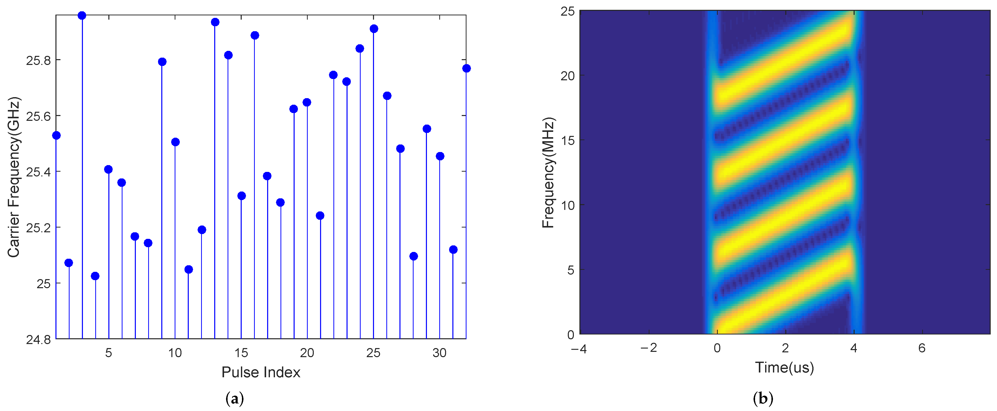
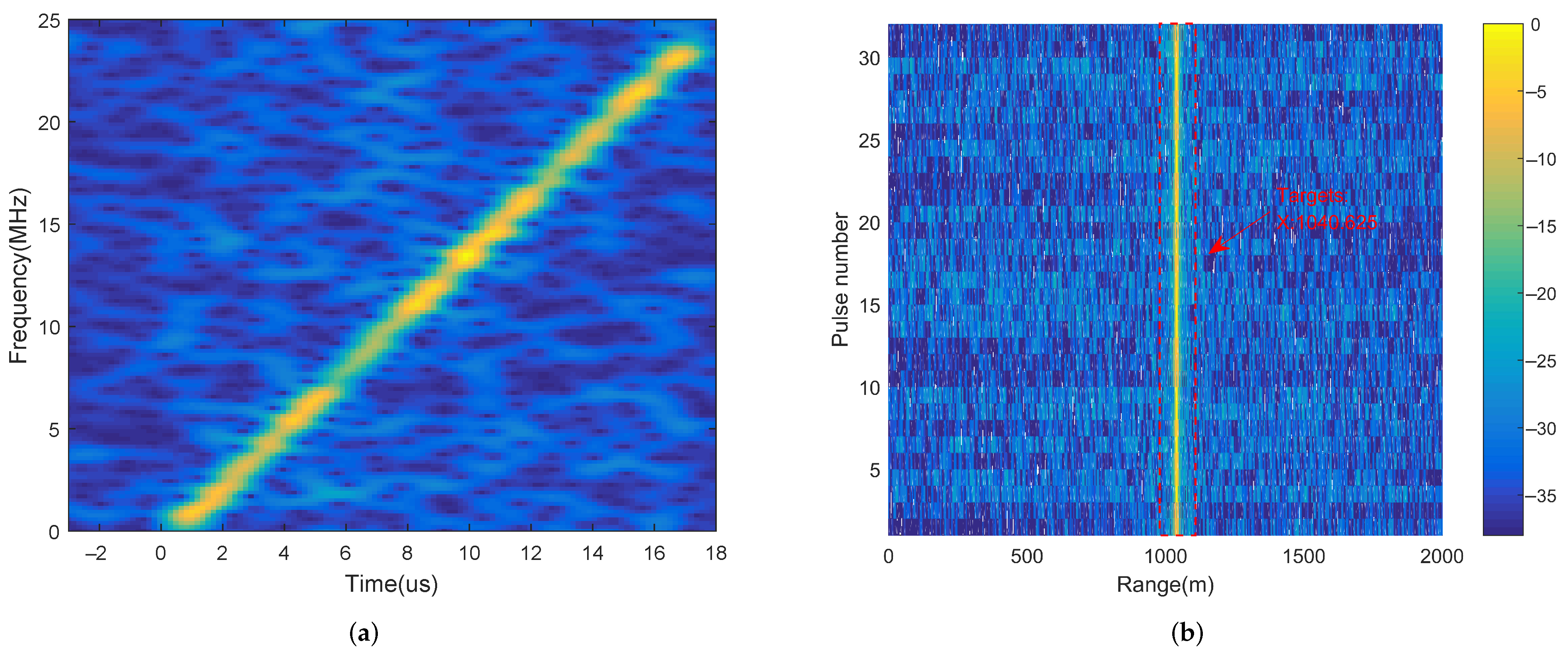
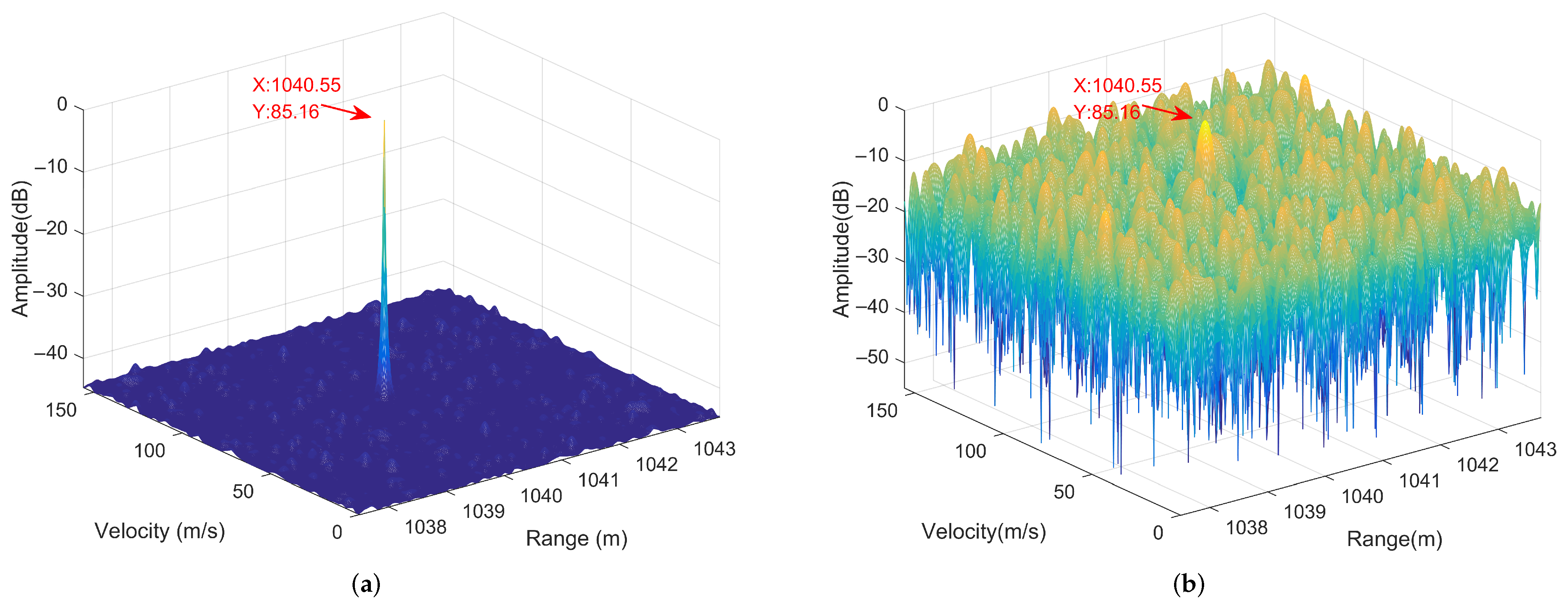
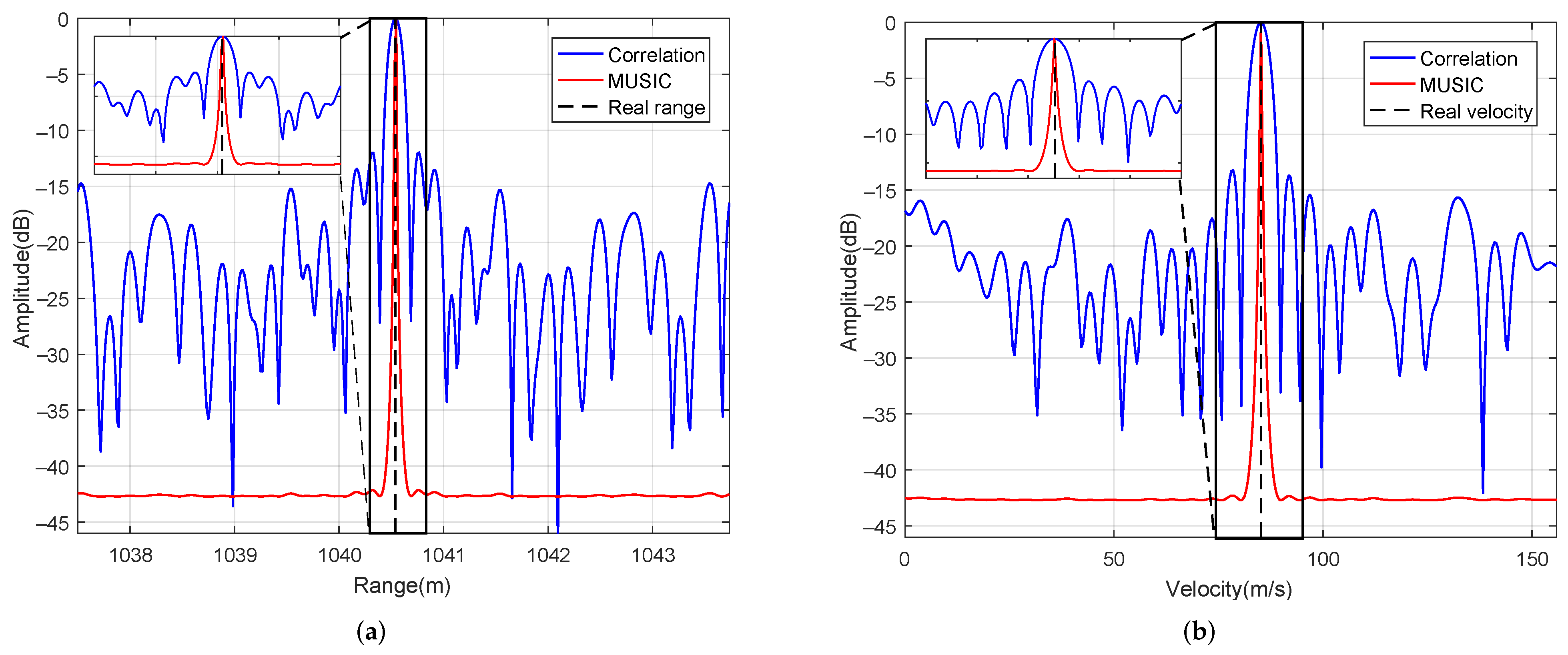
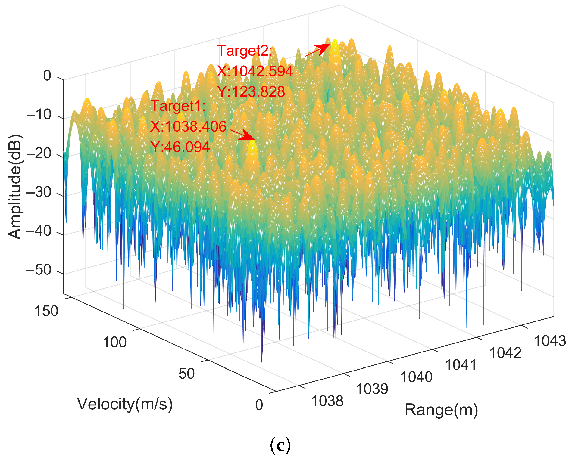
5.1. Signal Processing

After down-conversion, the method proposed in Section 3 is utilized to synthesize subcarriers. In Figure 4a, we can see that the four subcarriers are synthesized to obtain an LFM signal with bandwidth 24 MHz in the time domain. Therefore, the echo signal of the SFA-OFDM radar can be equivalent to that of the frequency agile radar mentioned in [30]. Moreover, compared to the subcarrier, the range resolution is improved. The range resolution is Δ R = c 2 B = 6.25 m, which is called the coarse range resolution in this paper. As shown in Figure 4a, after pulse compression, the coarse range of the target is R c = 1040.625 m. Thus, we can calculate the range ambiguity number, i.e., ε = R c R max = 1040.625 6.25 = 166 .
Next, we use the MUSIC algorithm to estimate the super-resolution range and velocity. Besides, for comparison, the correlation operation is also used. As depicted in Figure 5a, the proposed method can obtain the range and velocity of the moving target by searching over the range and velocity spaces. The estimated range is R m u s i c 3.05 m and the estimated velocity is 85.16 m/s by using the MUSIC algorithm. The target range can be determined by (28), i.e., R r e a l = 166 × 6.25 + 3.05 = 1040.55 m. The estimation error can be negligible. In Figure 5b, the correlation operation can also acquire the range and velocity with smaller error. To guarantee the same range and velocity resolution, we use the search matrix A ˜ to correlate with the echo signal. However, as shown in Figure 6, the columns of the search matrix are nonorthogonal which leads the range and velocity profile to generate higher sidelobes. Thus, weak targets are easily overwhelmed by the sidelobes. Moreover, the mainlobe of the correlation operation is also wider than that of the MUSIC algorithm.
Considering a multi-target scenario, we assume that the simulated scene consists of two moving targets as described in Table 2. The distance between the two targets is 4.1 m. As described in Figure 7a, due to the limitation of the coarse range resolution ( Δ R = 6.25 m), we can see that the two targets are in the same coarse range cell after pulse compression. The targets cannot be distinguished, and we only obtain a coarse range for the targets. As can be seen from Figure 7b, when the targets are in the same coarse range cell, the proposed method also obtains the super-resolution range and velocity estimations with smaller error (Target1 [1038.406 m, 46.094 m/s], Target2 [1042.594 m, 123.828 m/s]). In Figure 7c, the range and velocity of the different targets are obtained by using correlation operation. However, the sidelobes among the different targets will also be superimposed, which further causes sidelobes to rise.
To sum up, for the SFA-OFDM radar, the estimation method proposed in this paper can effectively realize the super-resolution range and velocity estimations. It overcomes the difficulty of coherent integration caused by frequency agility and provides a new idea to estimate the target parameters of the SFA-OFDM radar.

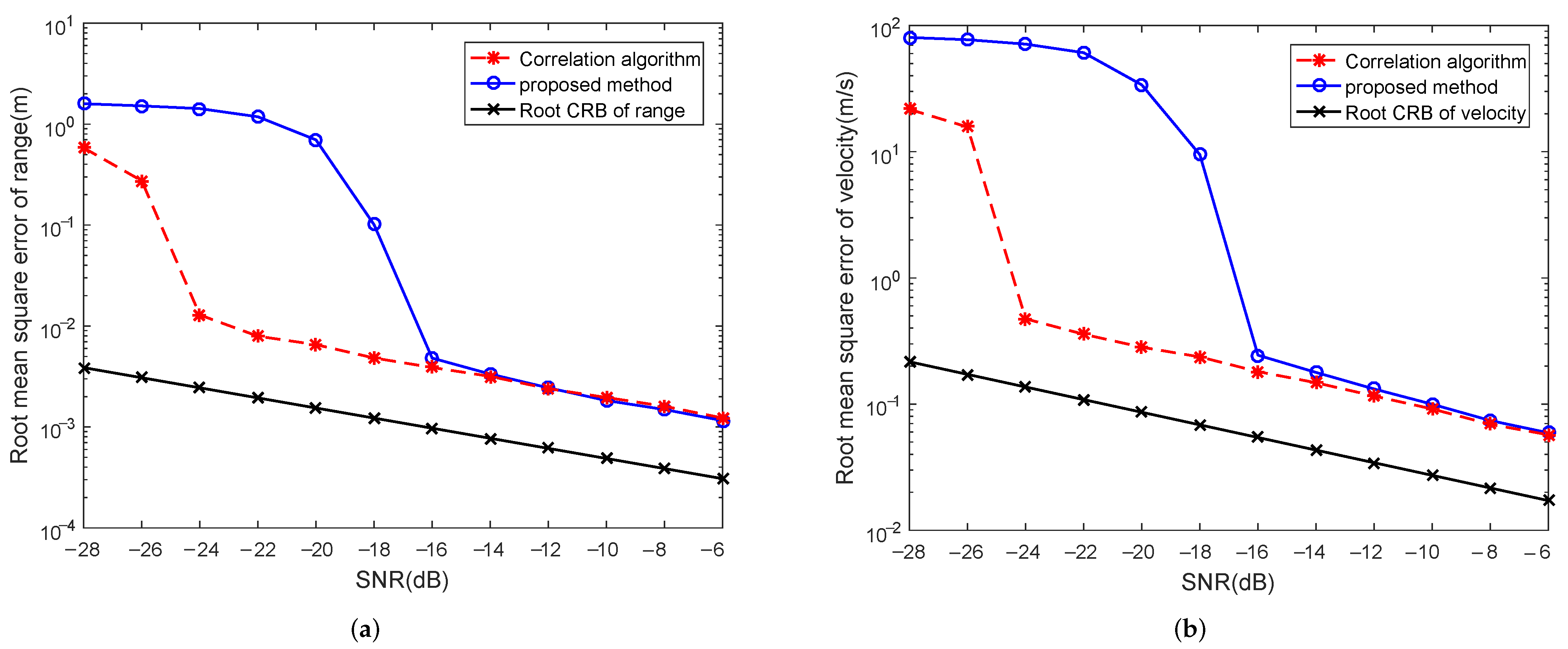
5.2. Estimation Performance

In this subsection, the range and velocity estimation performance of the proposed method is discussed. To obtain the root mean square errors (RMSEs) in the estimation of range and velocity, 500 independent Monte Carlo simulation experiments are conducted with different SNRs.
Figure 8a shows the RMSEs of the estimate of range versus SNR. For comparison, the RMSEs of range estimation by using the correlation algorithm is also investigated. It can be seen that when the SNR increases, the root CRLB and the RMSEs of range estimation decrease simultaneously. Under high SNR, the range estimation performance of the proposed method is similar to that of the correlation algorithm. Both methods can obtain high range estimation accuracy. However, when −24 dB < SNR < −16 dB, the estimation performance of the correlation algorithm is better than that of the proposed method. In other words, the correlation algorithm is more suitable for range estimation under the lower SNR circumstance. Meanwhile, we find that when the SNR decreases, the RMSE of range estimation increases sharply. This is called the threshold phenomenon [34]. The total MSE consists of the global MSE and the local MSE. When the probability of local MSE is less than 1, the threshold phenomenon will emerge. Similarly to Figure 8a, the RMSEs of velocity estimation are shown in Figure 8b, when SNR > −16 dB, the root CRLB on velocity estimation and the RMSEs of velocity estimation have the same varying tendency versus SNR and the proposed method and correlation algorithm have very close velocity estimation performance. Similarly to the range estimation performance, when −24 dB < SNR < −16 dB, the velocity estimation performance is worse than that of the correlation algorithm. Furthermore, when the SNR is further reduced, the threshold phenomenon will appear.

6. Conclusions

In this paper, to achieve the super-resolution range and velocity estimations simultaneously, a new signal processing scheme for the SFA-OFDM radar is investigated. It can effectively solve the problem of coherent integration caused by frequency agility. The subcarriers of each pulse are synthesized to an LFM signal at first. Then, the parameter estimations for the SFA-OFDM radar are equivalent to that of a linear array and the MUSIC algorithm is introduced to obtain the super-resolution range and velocity. The range–velocity resolution of the SFA-OFDM radar is only related to the size of the grid when the frequency hopping interval B is determined. Theoretical analyses and numerical experiments show that the proposed signal processing scheme can estimate the range and velocity of targets with small error. In future work, the communication information will be embedded in the varied frequencies to realize the integration of radar and communication. Moreover, the SFA-OFDM waveform will be used for super-resolution radar imaging, which can enhance the ECCM performance of the radar system while reducing the system complexity.

Author Contributions

Conceptualization, Z.L. and Y.Q.; methodology, Z.L.; software, Z.L.; validation, Y.Q. and M.X.; formal analysis, Y.W.; investigation, Z.L.; resources, Y.Q.; data curation, Z.L.; writing—original draft preparation, Z.L.; writing—review and editing, Z.L.; visualization, Z.L.; supervision, Y.Q.; project administration, Y.Q.; funding acquisition, Y.Q. All authors have read and agreed to the published version of the manuscript.

Funding

This work was supported by National Natural Science Foundation of China (61772397).

Institutional Review Board Statement

Not applicable.

Informed Consent Statement

Not applicable.

Data Availability Statement

The data is available to readers by contacting the corresponding author.

Acknowledgments

The author would like to thank the Institute of Advanced Remote Sensing Technology.

Conflicts of Interest

The authors declare no conflict of interest.

References

  1. Hwang, T.; Yang, C.; Wu, G.; Li, S.; Li, G.Y. OFDM and Its Wireless Applications: A Survey. IEEE Trans. Veh. Technol. 2009, 58, 1673–1694. [Google Scholar] [CrossRef]
  2. Siriwongpairat, W.; Su, W.; Olfat, M.; Liu, K.R. Multiband-OFDM MIMO coding framework for UWB communication systems. IEEE Trans. Signal Process. 2006, 54, 214–224. [Google Scholar] [CrossRef]
  3. Wang, M.M.; Xiao, L.; Brown, T.; Dong, M. Optimal symbol timing for OFDM wireless communications. IEEE Trans. Wirel. Commun. 2009, 8, 5328–5337. [Google Scholar] [CrossRef]
  4. Wang, J.; Zhang, B.; Lei, P. Ambiguity function analysis for OFDM radar signals. In Proceedings of the 2016 CIE International Conference on Radar (RADAR), Guangzhou, China, 10–13 October 2016; pp. 1–5. [Google Scholar] [CrossRef]
  5. Demeechai, T.; Chang, T.G.; Siwamogsatham, S. Performance of a Frequency-Domain OFDM-Timing Estimator. IEEE Commun. Lett. 2012, 16, 1680–1683. [Google Scholar] [CrossRef]
  6. Zhang, T.; Xia, X.G. OFDM Synthetic Aperture Radar Imaging With Sufficient Cyclic Prefix. IEEE Trans. Geosci. Remote Sens. 2015, 53, 394–404. [Google Scholar] [CrossRef] [Green Version]
  7. Slimane, Z.; Abdelmalek, A.; Feham, M. OFDM Based UWB Synthetic Aperture Through-wall Imaging Radar. In Proceedings of the 2008 Third International Conference on Broadband Communications, Information Technology Biomedical Applications, Pretoria, South Africa, 23–26 November 2008; pp. 293–300. [Google Scholar] [CrossRef]
  8. Sen, S.; Tang, G.; Nehorai, A. Multiobjective Optimization of OFDM Radar Waveform for Target Detection. IEEE Trans. Signal Process. 2011, 59, 639–652. [Google Scholar] [CrossRef]
  9. Chabriel, G.; Barrère, J. Adaptive Target Detection Techniques for OFDM-Based Passive Radar Exploiting Spatial Diversity. IEEE Trans. Signal Process. 2017, 65, 5873–5884. [Google Scholar] [CrossRef] [Green Version]
  10. Liu, Y.; Liao, G.; Chen, Y.; Xu, J.; Yin, Y. Super-Resolution Range and Velocity Estimations With OFDM Integrated Radar and Communications Waveform. IEEE Trans. Veh. Technol. 2020, 69, 11659–11672. [Google Scholar] [CrossRef]
  11. Chiriyath, A.R.; Ragi, S.; Mittelmann, H.D.; Bliss, D.W. Novel Radar Waveform Optimization for a Cooperative Radar-Communications System. IEEE Trans. Aerosp. Electron. Syst. 2019, 55, 1160–1173. [Google Scholar] [CrossRef]
  12. Cao, N.; Chen, Y.; Gu, X.; Feng, W. Joint Radar-Communication Waveform Designs Using Signals From Multiplexed Users. IEEE Trans. Commun. 2020, 68, 5216–5227. [Google Scholar] [CrossRef]
  13. Huo, K.; Deng, B.; Liu, Y.; Jiang, W.; Mao, J. The principle of synthesizing HRRP based on a new OFDM phase-coded stepped-frequency radar signal. In Proceedings of the IEEE 10th International Conference on Signal Processing Proceedings, Beijing, China, 24–28 October 2010; pp. 1994–1998. [Google Scholar] [CrossRef]
  14. Schweizer, B.; Knill, C.; Schindler, D.; Waldschmidt, C. Stepped-Carrier OFDM-Radar Processing Scheme to Retrieve High-Resolution Range-Velocity Profile at Low Sampling Rate. IEEE Trans. Microw. Theory Tech. 2018, 66, 1610–1618. [Google Scholar] [CrossRef] [Green Version]
  15. Nuss, B.; Mayer, J.; Marahrens, S.; Zwick, T. Frequency Comb OFDM Radar System With High Range Resolution and Low Sampling Rate. IEEE Trans. Microw. Theory Tech. 2020, 68, 3861–3871. [Google Scholar] [CrossRef]
  16. Nuss, B.; de Oliveira, L.G.; Zwick, T. Frequency Comb MIMO OFDM Radar With Nonequidistant Subcarrier Interleaving. IEEE Microw. Wirel. Components Lett. 2020, 30, 1209–1212. [Google Scholar] [CrossRef]
  17. Quan, Y.; Wu, Y.; Li, Y.; Sun, G.; Xing, M. Range–Doppler reconstruction for frequency agile and PRF-jittering radar. IET Radar Sonar Navig. 2018, 12, 348–352. [Google Scholar] [CrossRef]
  18. Huang, P.; Dong, S.; Liu, X.; Jiang, X.; Liao, G.; Xu, H.; Sun, S. A Coherent Integration Method for Moving Target Detection Using Frequency Agile Radar. IEEE Geosci. Remote Sens. Lett. 2019, 16, 206–210. [Google Scholar] [CrossRef]
  19. Huang, T.; Liu, Y.; Xu, X.; Eldar, Y.C.; Wang, X. Analysis of Frequency Agile Radar via Compressed Sensing. IEEE Trans. Signal Process. 2018, 66, 6228–6240. [Google Scholar] [CrossRef] [Green Version]
  20. Lellouch, G.; Pribic, R.; van Genderen, P. OFDM waveforms for frequency agility and opportunities for Doppler processing in radar. In Proceedings of the 2008 IEEE Radar Conference, Rome, Italy, 26–30 May 2008; pp. 1–6. [Google Scholar] [CrossRef]
  21. Lellouch, G.; Pribic, R.; van Genderen, P. Frequency agile stepped OFDM waveform for HRR. In Proceedings of the 2009 International Waveform Diversity and Design Conference, Kissimmee, FL, USA, 8–13 February 2009; pp. 90–93. [Google Scholar] [CrossRef]
  22. Long, X.; Li, K.; Tian, J.; Wang, J.; Wu, S. Ambiguity Function Analysis of Random Frequency and PRI Agile Signals. IEEE Trans. Aerosp. Electron. Syst. 2021, 57, 382–396. [Google Scholar] [CrossRef]
  23. Knill, C.; Schweizer, B.; Sparrer, S.; Roos, F.; Fischer, R.F.H.; Waldschmidt, C. High Range and Doppler Resolution by Application of Compressed Sensing Using Low Baseband Bandwidth OFDM Radar. IEEE Trans. Microw. Theory Tech. 2018, 66, 3535–3546. [Google Scholar] [CrossRef] [Green Version]
  24. Knill, C.; Schweizer, B.; Stephany, S.; Werbunat, D.; Waldschmidt, C. FMCW-Interference of Frequency Agile OFDM Radars. In Proceedings of the 2020 17th European Radar Conference (EuRAD), Utrecht, The Netherlands, 10–15 January 2021; pp. 160–163. [Google Scholar] [CrossRef]
  25. Knill, C.; Schweizer, B.; Waldschmidt, C. Interference-Robust Processing of OFDM Radar Signals Using Compressed Sensing. IEEE Sens. Lett. 2020, 4, 1–4. [Google Scholar] [CrossRef]
  26. Rida, I.; Al-Maadeed, S.; Mahmood, A.; Bouridane, A.; Bakshi, S. Palmprint Identification Using an Ensemble of Sparse Representations. IEEE Access 2018, 6, 3241–3248. [Google Scholar] [CrossRef]
  27. Schmidt, R. Multiple emitter location and signal parameter estimation. IEEE Trans. Antennas Propag. 1986, 34, 276–280. [Google Scholar] [CrossRef] [Green Version]
  28. Cheng, F.; He, Z.; Liu, H.; Li, J. The parameter setting problem of signal OFDM-LFM for MIMO radar. In Proceedings of the 2008 International Conference on Communications, Circuits and Systems, Xiamen, China, 25–27 May 2008; pp. 876–880. [Google Scholar] [CrossRef]
  29. Lord, R.; Inggs, M. High range resolution radar using narrowband linear chirps offset in frequency. In Proceedings of the 1997 South African Symposium on Communications and Signal Processing, COMSIG ’97, Grahamstown, South Africa, 9–10 September 1997; pp. 9–12. [Google Scholar] [CrossRef]
  30. Li, Y.; Huang, T.; Xu, X.; Liu, Y.; Wang, L.; Eldar, Y.C. Phase Transitions in Frequency Agile Radar Using Compressed Sensing. IEEE Trans. Signal Process. 2021, 69, 4801–4818. [Google Scholar] [CrossRef]
  31. Zoltowski, M. Synthesis of sum and difference patterns possessing common nulls for monopulse bearing estimation with line arrays. IEEE Trans. Antennas Propag. 1992, 40, 25–37. [Google Scholar] [CrossRef]
  32. Friedlander, B. A sensitivity analysis of the MUSIC algorithm. IEEE Trans. Acoust. Speech Signal Process. 1990, 38, 1740–1751. [Google Scholar] [CrossRef]
  33. Kay, S.M. Fundamentals of Statistical Signal Processing: Estimation and Detection Theory; PRT Prentice Hall: Englewood Cliffs, NJ, USA, 1993. [Google Scholar]
  34. Trees, H.L.V. Optimum Array Processing: Part IV of Detection, Estimation, and Modulation Theory; Wiley: Hoboken, NJ, USA, 2004. [Google Scholar]
Figure 1. SFA-OFDM radar signal model in the time–frequency domain.
Remotesensing 14 00278 g001
Figure 2. Block diagram of subcarrier synthesis processing.
Remotesensing 14 00278 g002
Figure 3. (a) Sequence of carrier frequency. (b) SFA-OFDM radar signal in the time–frequency domain.
Remotesensing 14 00278 g003
Figure 4. (a) The result of subcarrier synthesis processing in the time–frequency domain. (b) Pulse compression after subcarrier synthesis processing.
Remotesensing 14 00278 g004
Figure 5. Signal processing results for the moving target. (Target [1040.54 m, 85.2 m/s]). Range–velocity profile using (a) MUSIC algorithm (b) correlation operation.
Remotesensing 14 00278 g005
Figure 6. Range and velocity profiles (a) Range profile at 1040.54 m. (b) Velocity profile at 85.2 m/s.
Remotesensing 14 00278 g006
Figure 7. The results of signal processing for two targets: (a) Pulse compression and range and velocity estimations using (b) MUSIC algorithm and (c) correlation operation (Target1 [1038.4 m, 46 m/s], Target2 [1042.6 m, 124 m/s]).
Remotesensing 14 00278 g007aRemotesensing 14 00278 g007b
Figure 8. RMSEs of range and velocity estimations. (a) RMSEs in the estimation of range. (b) RMSEs in the estimation of velocity.
Remotesensing 14 00278 g008
Table 1. Parameters of SFA-OFDM radar.
Parameter (Unit)SymbolValue
Number of subcarriersK4
Number of pulsesM32
Total number of available frequenciesN40
Pulse width (us) T p 4
Pulse repetition interval (us) T r 40
Subcarrier bandwidth (MHz) Δ f 6
Frequency hopping interval (MHz)B24
Chirp rate (MHz/us) γ 1.5
Lowest carrier frequency (GHz) f 0 24
Sample rate (MHz) f s 24
Table 2. Parameters for the moving targets.
TargetRange (Unit)Velocity (Unit)
Target11038.4 m46 m/s
Target21042.6 m124 m/s
Publisher’s Note: MDPI stays neutral with regard to jurisdictional claims in published maps and institutional affiliations.

