Article

Classification of Land-Water Continuum Habitats Using Exclusively Airborne Topobathymetric Lidar Green Waveforms and Infrared Intensity Point Clouds

1
Coastal GeoEcology Lab, Ecole Pratique des Hautes Etudes—PSL Université, 35800 Dinard, France
2
UMR 6554 LETG, Université Rennes 2, CNRS, 35000 Rennes, France
3
Géosciences Rennes—UMR 6118, Univ Rennes, CNRS, 35000 Rennes, France
4
Service Hydrographique et Océanographique de la Marine, 29200 Brest, France
5
Airborne Hydrography AB, 553 03 Jonkoping, Sweden
*
Author to whom correspondence should be addressed.
Remote Sens. 2022, 14(2), 341; https://doi.org/10.3390/rs14020341
Submission received: 15 November 2021 / Revised: 3 January 2022 / Accepted: 7 January 2022 / Published: 12 January 2022

Abstract

:
Coastal areas host highly valuable ecosystems that are increasingly exposed to the threats of global and local changes. Monitoring their evolution at a high temporal and spatial scale is therefore crucial and mostly possible through remote sensing. This article demonstrates the relevance of topobathymetric lidar data for coastal and estuarine habitat mapping by classifying bispectral data to produce 3D maps of 21 land and sea covers at very high resolution. Green lidar full waveforms are processed to retrieve tailored features corresponding to the signature of those habitats. These features, along with infrared intensities and elevations, are used as predictors for random forest classifications, and their respective contribution to the accuracy of the results is assessed. We find that green waveform features, infrared intensities, and elevations are complimentary and yield the best classification results when used in combination. With this configuration, a classification accuracy of 90.5% is achieved for the segmentation of our dual-wavelength lidar dataset. Eventually, we produce an original mapping of a coastal site under the form of a point cloud, paving the way for 3D classification and management of land and sea covers.

Graphical Abstract

1. Introduction

Monitoring coastal areas is essential to the preservation of the land-water continuum’s habitats and the services they provide, particularly in a context of local and global changes [1]. Seagrasses, salt marshes, mangroves, macroalgae, sandy dunes, or beaches are examples of such habitats that continually interact with the tide levels. They can be found along the temperate shorelines and play key roles in the ecological equilibrium of these ecotones. Seagrasses ensure water quality and are a significant carbon sink, along with salt marshes and mangroves [1,2]. Coastal habitats also provide protection from marine hazards to coastal communities and infrastructures and supply many recreational activities such as snorkeling, fishing, swimming, and land sailing [1,2,3]. Finally, they support a wide range of endemic species by offering them nurseries, food, and oxygen [1,2]. However, coastal (including estuarine) habitats are exposed to a plethora of natural and anthropic threats that may be amplified by global changes. Thorough observation of coastal processes is necessary to identify the trends of evolution of these fragile environments. It requires regular data acquisition along the shoreline with spatial resolution and time spacing both adapted to the task. However, the surveying complexities inherent to land-water continuum areas hinder their monitoring at a time scale relevant to their fast evolution, and over large, representative extents. Remote sensing can adequately address this issue.
Due to the presence of water, coastal surveys are conventionally split between topographic and bathymetric campaigns, both constrained to the tide and the field accessibility. Subtidal areas can be surveyed with waterborne acoustic techniques, while supratidal domains are documented with passive or active imagery using satellite, airborne, or unmanned aerial vehicles (UAV) [4,5,6]. Boats being unable to reach very shallow areas and imagery being limited by the water surface, intertidal, and shallow water areas are harder to accurately monitor [7]. Distinct terrestrial and marine surveying campaigns can also be difficult to merge, considering they might rely on different reference systems, and their thin overlapping area can be challenging to sample thoroughly with ground control points. Existing seamless surveying techniques over land-water interface areas are summarized in the following section.
Multispectral or superspectral imagery can be used for coastal habitat mapping. In clear and shallow water, traditional image classification techniques can be applied [7]. A more accurate approach consists in suppressing the effects of water on light refraction and diffusion by using inversion models on superspectral imagery. Using such models, it is possible to obtain satellite-derived bathymetry [8] or satellite-derived topobathymetry [9,10], which are proven to improve the classification of coastal covers obtained [11]. Bathymetry can also be extracted using multispectral imagery, as demonstrated in [12]. Multispectral imagery has the advantage of being accessible with different platforms: UAVs, planes, or satellites nowadays all benefit from multiband sensors. The cost of acquisition can therefore be lowered depending on the chosen source, and the revisit time can allow high temporal resolution monitoring.
Hyperspectral imagery is the last passive imagery-based method to map the land-water continuum [13,14]. The key principle of methods using hyperspectral imagery to study submerged areas is to model the interactions of light with the water column and correct them to obtain imagery unaffected by these processes. By inversing a radiative transfer model of the water column, it is possible to derive the seafloor reflectance and estimate the bathymetry [15]. These products are adapted to the characterization of sea bottom types and can be used for benthic classification tasks.
Although satellite passive imagery overcomes the issue of accessibility and temporal resolution, its spatial resolution is sometimes too coarse to spot specific changes (depending on the sensor and the quality of pan-sharpening), and it only penetrates water in shallow, clear areas [16]. The main issue with passive imagery remains the depth range in which it is usable. Due to optical phenomena, past a certain depth threshold that varies with water clarity, passive imagery can no longer give information on what lies beneath the water surface. Bathymetry extraction via active imaging then becomes the only way to gather information on these areas. Furthermore, even in shallow waters, bathymetry derived from active sensors gives access to the seabed covers’ elevation but also to the seabed’s elevation itself, providing 3D information on these covers, which enables biomass estimation or other structural assessments [17,18,19,20]. The bathymetry measurements obtained with active sensors (airborne bathymetric lidar or waterborne acoustic soundings) also leverage a higher vertical precision, useful for ecological structural assessments [12].
Airborne topobathymetric lidar is a reliable alternative: it ensures information continuity between land and water, covers vast areas quickly, penetrates a depth of up to dozens of meters and has a higher spatial resolution than satellite imagery [21,22]. Current approaches to map coastal interfaces using airborne lidar mostly make use of the digital terrain models or digital surface models derived from the lidar point clouds (PCs), including those obtained for the water bottoms after removing points corresponding to the water bodies [17]. Fewer studies rely on the 3D PCs of the lidar surveys to generate coastal or riverside habitats maps. Directly processing the PCs and avoiding rasterization has the advantage of preserving the dense spatial sampling provided by lidar sensors. It also opens possibilities for 3D rendering of the results, and structural analysis thanks to the rich spatial information contained in PCs. Indeed, the vertical repartition of the points offers useful information on scene architecture, providing relevant features to determine their origin, namely for vegetation or building identification. Analysis of this geometrical context is the most frequently used method to produce maps of land and water covers [23,24,25]. Research works conducted on PCs processing mostly rely on the computation of geometrical features using spherical neighborhoods [23] and, more recently, on deep neural networks [26].
Another possibility with airborne lidar is to exploit the spectral details contained in the backscattered signals. These can be recorded under the form of time series of intensities received by the sensor: lidar waveforms. Each object of the surveyed environment illuminated by the sensor’s laser reflects light in a specific way, generating a characteristic signature in the signal. Waveforms consequently provide additional information on the structure and physical attributes of the targets. The shape, width, and amplitude of their spectral signature—a peak—are information that can be used for land and water covers mapping [27,28,29]. Waveforms are therefore a useful indicator of the diversity of coastal areas. Though many methods have been proposed to process airborne topographic lidar full-waveforms, airborne bathymetric lidar full-waveforms are, to the best of our knowledge, much less explored. They are even less employed for classification tasks, and often only analyzed to retrieve bathymetry. There are currently three main approaches to waveform processing. The first consists in decomposing the waveforms to isolate each element of the train of echoes in the signal [30,31]. The second consists in reconstructing the signal by fitting statistical models to the waveforms [32]. Knowing how to approximate the sensed response allows to extract the position and the attributes of each component. The last approach is to analyze waveforms straightforwardly as any 1D signal to detect their peaks [27], using first derivative thresholding for example. Identifying waveform components is useful in order to localize the objects populating the scene, but also to extract features to describe them and prepare their automatic classification [27,33,34].
Classification of land or water covers using lidar data has been well explored recently. Even when using waveform data, most of the published research is based on 2D data classification [17,25,27,29,33] while fewer articles exploit PCs [24,34,35]. Many studies researching ways to classify lidar data used machine learning algorithms such as support vector machine (SVM), maximum likelihood (ML), or random forests. The maximum likelihood is mostly used for 2D lidar data, while SVM and random forests have been proofed on PCs. SVM and random forest seem to have similar classification performances on 3D lidar data [36]. However, with these algorithms, the spatial context around each point is not considered and does not impact the prediction [36]. Research papers show that conditional random field (CRF) and Markov random field (MRF) classifications produce better results in that way [36,37]. However, these require heavier computation and are more difficult to apply to large datasets. Currently, there is a consensus on the efficiency of random forest on that aspect [36]. Contrary to SVM, CRF, or MRF, it is easy to apply to large datasets. Random forest is, furthermore, robust to overfitting issues and offers the possibility to retrieve predictors contribution easily. In this article, we therefore wish to implement a hand-crafted features’ random forest classification to map coastal habitats. Although machine learning classification of lidar waveform features has been explored previously, we have found no point-based studies dedicated to mapping a large number of habitats both marine and terrestrial. Previously cited studies such as [24,34,35] classified either only marine or only terrestrial habitats from PCs and [27] processed 2D data to produce their map of coastal habitats.
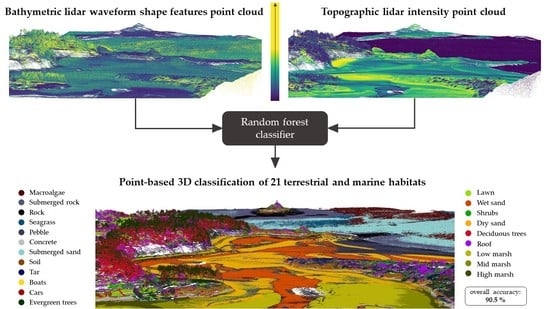
The present study aims at mapping an array of 21 habitats of the 3D land-water continuum seamlessly using exclusively airborne topobathymetric bispectral lidar. Our objective is to bridge the gap between marine and terrestrial surveys, demonstrate that efficient methods can be developed to automatically map the land-water interface, and show that an integrated vision of coastal zones is feasible and advised. Our contributions consist in (1) developing a point-based approach to exploit full-waveform data acquired during topobathymetric surveys for subtidal, intertidal, and supratidal habitats mapping, (2) quantifying the contribution of green waveform features, infrared (IR) intensities, and relief information to the classification accuracy based on a random forest machine learner. We improve an experimental method presented in a previous work [29] and test it on a wider area including both emerged and submerged domains to determine the suitability of full-waveform lidar data for coastal zone mapping. UAV data, inexpensive to implement, is used to estimate the accuracy of the resulting very high spatial resolution maps, which are produced under the form of PCs, paving the way for 3D classification of land and sea covers using solely topobathymetric lidar data.

2. Materials

2.1. Study Area

The study location was chosen along the northern coasts of Brittany, France, for its ecological diversity and due to the availability of full-waveform lidar data acquired by the French Hydrographic Office (Shom) as part of the Litto3D® project [38]. The study area, presented in Figure 1, features typical coastal habitats such as fine sand or pebble beaches, a sandy dune, rocky areas provided with macroalgae, seagrass meadows, and salt marshes at the estuary of a local river. It also hosts a small resort town, Sables d’Or les Pins (48°38′27′′N: 2°24′24′′W). Buildings, tar or concrete-covered paths, boats in mooring, vehicles in parking lots, wooded areas populated with evergreen pine trees or deciduous species, and crop fields are also present in the selected zone. All these habitats are home to a rich variety of species: shellfish; dune plant vegetation; green, red, and brown seaweed; eelgrasses; evergreen and deciduous trees; crops; and salt marsh plants such as glasswort, common soda, sea purslane, or sea lavender.

2.2. Full-Waveform Airborne Topobathymetric Lidar

Airborne lidar is an active remote sensing technique that uses the backscatter of laser light in the environment to compute ranges to the ground cover and produce 3D maps of the environment, knowing the absolute position of the sensor. Topobathymetric lidar relies on two different lasers with distinct wavelengths: a green laser is added to the usual IR laser to detect the seabed or riverbed [21,22,39]. It exploits the physical properties of the green spectrum that penetrates the water surface, whereas the IR light does not. Lidar waveform is the recording of the full backscattered signal on the surveyed environment. A waveform consists in samples of recorded backscattered intensities over time. Since laser light is reflected by objects standing on its path, each element illuminated by the lidar laser backscatters a fraction of the emitted beam, which results in a peak in the waveform. Peaks are theoretically more or less intense depending on the object’s albedo, its geometry and the laser incidence angle [40]. Due to the different layers of coverage in the environment (tree canopy, tree branches, bushes, soils, for example), there can be several peaks in the same waveform, all corresponding to a different layer in the reality. A typical topographic waveform (i.e., resulting from a laser beam hitting the land) has as many peaks as there are objects of different elevation in its way [28,39]. A bathymetric waveform usually has three main components: the first is the water surface return, the second is the water column return (originating from the backscatter of photons on particles suspended in the water such as sediments or nutrients), and the third is the return originating from the reflection on the seabed or riverbed [21,22,39]. Since all objects present in the cone illuminated by the laser reflect some light towards the sensor, they all contribute to the recorded waveform’s shape [28]. Each element of the landscape/seascape is therefore characterized by the shape of its component in the waveform, which can be used for land or sea cover detection and classification [27,29,34,41]. In this work, backscattered intensities are converted into pseudo-reflectances by dividing them with the emitted pulse’s intensity. Examples of a typical bathymetric waveform and a typical topographic waveform are presented in Figure 2.

2.3. Datasets

The lidar data [42] used for this research were acquired over the coast of Sables d’Or les Pins in September 2019 by the Shom as part of the Litto3D® project [38], using a Leica HawkEye 4X sensor. The HawkEye 4X produces laser pulses at wavelengths of 515 nm and 1064 nm on three different channels. Depths under 10 m have a dedicated shallow green laser, while a more powerful laser, the deep channel, is used to detect deeper seabed. These two channels provide PCs with a density of at least five points per m² and one point per m² and they have a laser spot size diameter of 1.8 m and 3.4 m, respectively. The IR laser has a laser spot size of 0.2 m and a point density of at least 10 points per m². For green channels only, backscattered intensities are recorded with a time frequency of 1.8 GHz, providing waveforms with a sample every 556 picoseconds. This information is not available for the IR laser.
The survey was conducted with a constant laser amplification. Due to the power needed to penetrate through several meters of water, the shallow laser’ backscattered intensities tend to be saturated over highly reflective land surfaces, but they are still usable. The deep channel’s returned intensities, however, are systematically saturated and do not provide usable information for land cover classification. In this study, only shallow full waveforms were used, considering the selected area’s range of depths. The green waveforms used were available for every shallow green laser shot. Over the studied area, their average density was 3.75 waveforms per m². Reanalyzed echo PCs for both shallow green and IR wavelengths were also used: the IR PC brought additional spectral information, while the green PC was used to accurately position the raw waveforms, since this PC underwent refraction correction before delivery. The effects of refraction were not corrected in the raw waveform files.
To provide knowledge on the environment on site, ground truth data (presented in Figure 3) were acquired in the form of photoquadrats and UAV imagery. They helped label the lidar data to perform habitat classification. UAV imagery was acquired over five smaller areas of interest, each representing typical coastal habitats, in March and April 2021 using an RGB DJI Phantom 4 Pro V2, and a Parrot Sequoia+ including a near IR nadiral sensor (770 nm to 810 nm) with a zenithal irradiance sensor. These flights were calibrated with a total of 55 ground control points. An array of 150 photoquadrats were captured with RGB cameras and georeferenced, to seize the ecological diversity of the study area. Over marine parts of the study site, a PowerVision unmanned surface vehicle (USV) was used to gather knowledge of the seabed covers. The underwater images were acquired in September 2021. An RGB orthoimage acquired in 2014 over the whole area was also used to give extra information on the habitats present on site four years prior to the data acquisition.

3. Methodology

The algorithm developed in this study was first introduced in [29] to identify marine habitats using green full-waveform spectral features. In [29], only seagrasses and sediments (two classes) at few meters’ depths were classified. We significantly improved this algorithm and adapted it to the classification of 21 habitats across the land-water interface, to test its abilities in supratidal and intertidal environments.
The enhanced version presented here was tailored to the identification of land and sea covers: the seabed or riverbed type was considered in the presence of water while we focused on the surface cover over terrestrial areas (i.e., if there were two layers of surface covers, such as a trees and grass beneath it, the land cover was labelled as tree). It used a supervised point-based classification algorithm trained on various sets of input features and evaluated on a test dataset. Classified PCs of the whole area were also produced to observe the ability of each predictor sets to produce a map of the habitats in the study area using this approach.

3.1. Classes of Land and Sea Covers Investigated

A total of 21 classes of land and sea covers has been designed based on on-site observations and photo-interpretation. These classes are illustrated in Table 1.

3.2. Data Pre-Processing

The classification algorithm developed for this research aimed at processing bispectral lidar data. Two PCs were therefore used, but full-waveforms were available only for the green wavelength. IR data were thus incorporated as reflected intensities only. Due to the sensor’s configuration, IR and green lasers of the topobathymetric lidar used are not co-focal. They also do not have the same swath, density, and precision. The two resulting PCs are consequently different, and the points acquired do not have identical locations. A preprocessing step was therefore required to obtain the IR backscattered intensity at each green waveform’s location. Intensities of the IR PC were matched with each point of the green waveforms PC, which was kept as the reference PC, using the median IR intensity of the 10 nearest neighbors of each green waveform’s location in the IR PC, which was computed and assigned to the waveform as an attribute. To this end, we used the PC processing software “CloudCompare” [43], in which the neighborhood search is performed by computing the 3D Euclidean distance between each point of the reference PC and the points of the compared PC. The coordinates of the waveforms’ cover component were used to locate each waveform and obtain a green waveform PC. Consequently, each waveform was synthesized as a point, and we obtained a green waveforms PC. The IR PC was cleaned manually beforehand, to ensure all noise points, significantly above the surface, were removed from the data.
The median intensity of the 10 closest neighbors in the IR PC was chosen for two reasons. First, the number of 10 neighbors was relevant considering the difference of the two lasers’ spot sizes and the resulting density of the PCs. Second, the use of the median intensity was more suited to the task than the mean intensity to avoid outliers’ artefacts in spheres located at the interface of two habitats.

3.3. Training and Testing Datasets

Two main datasets were designed to perform the data classifications and assess their quality, called the training dataset and test dataset. We collected 1000 training and 500 testing samples of each class. To do so, we first drew polygons over representative areas of the 21 land and water covers, based on the ground-truth data, and made sure none of the polygons intersected. We used these to segment the PC and extract points located within representative areas of each class. For each class, we then randomly selected 1000 of them for the training datasets and 500 others for testing, which resulted in training and test datasets of 21,000 and 10,500 items, respectively. This draw without replacement ensured that no training and testing points were the same and that they were all independent. We chose to use the same areas for random drawing of training and testing points in order to account for the widest diversity possible in the training and testing samples. The resulting training and test points have a mean distance of 1.6 m; their repartition is presented in Figure 4.
Each array of coordinates, IR intensities, and waveform features was associated to one integer label between 1 and 21, forming a dataset with the structure illustrated in Figure 5.
The point-based classification method is described in the following paragraphs. It relied on the interpolated IR intensities and on spectral features extracted from the green waveforms.

3.4. Waveform Processing Method

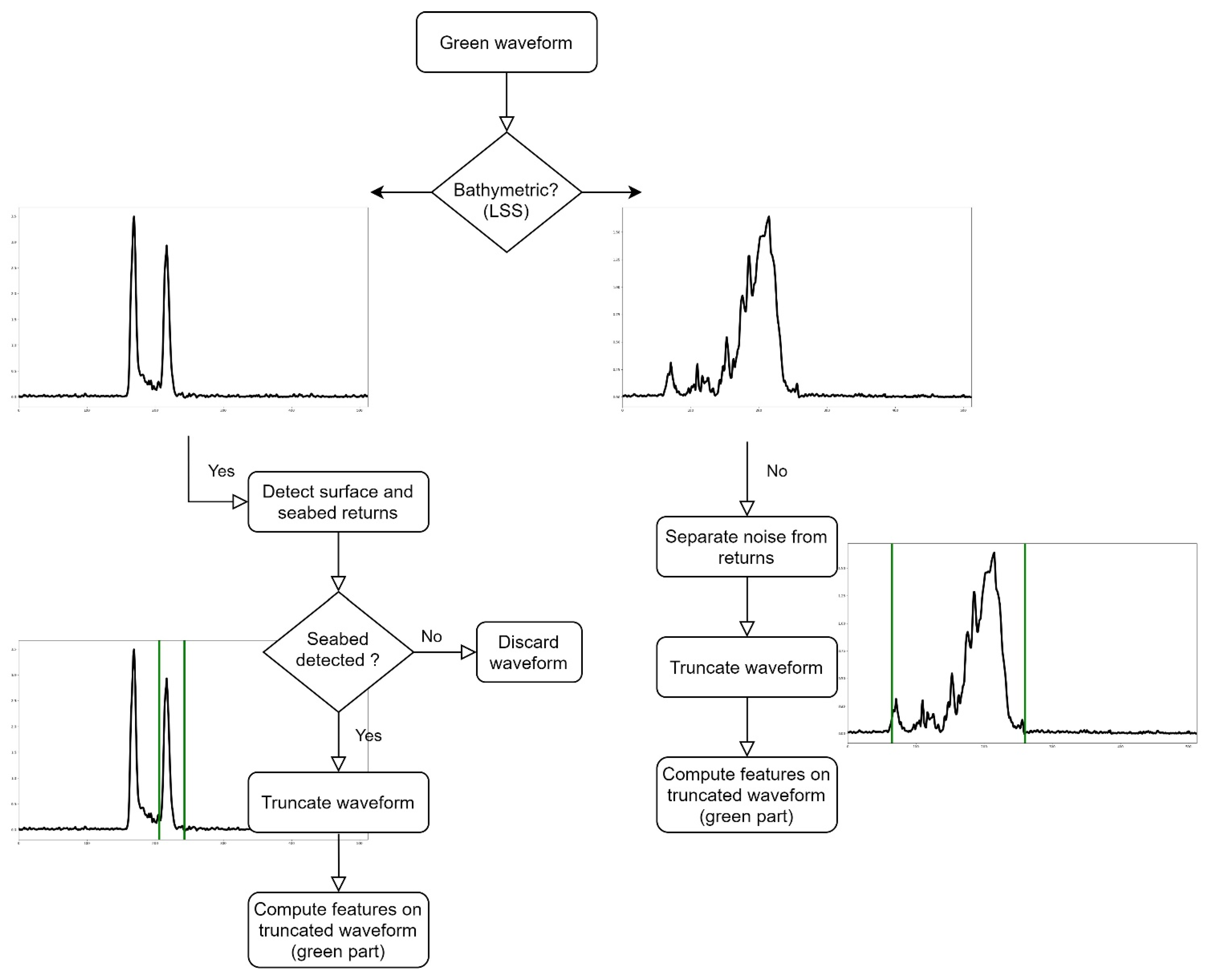
The waveform processing steps are presented in Figure 6 and detailed in the following paragraphs. All these steps were performed using tailored scripts developed with Python 3.8.8.
The base concept consists in extracting tailored features from the relevant part of the waveforms. Here, we considered this part to be any return detected after the water surface component in submerged domains, and the part of the waveform encompassing the backscattered signal in terrestrial zones. In these zones, the sole processing was to isolate the useful part of the green waveform by identifying where the backscatter begins and the noise ends. This was made by evaluating the mean level of noise observable at the beginning and at the end of the waveform and extracting the part of the wave where the intensity was above this noise level.
To distinguish marine and terrestrial waveforms, we relied on a flag attributed by the Leica survey software Leica LIDAR Survey Studio (LSS) to points in the PC that correspond to an interpolated water surface under which refraction correction is made. Since waveform files integrate this information, it was possible to use it to differentiate submerged and emerged areas. This step is a pre-classification made by LSS before the data was delivered to us.
In submerged areas, further processing was required to detect the different peaks and isolate the parts of the signal that correspond to the water surface and the water column components. All green waveforms were first filtered using the Savitzky–Golay piecewise polynomial functions estimation method to remove the noise. As explained in [29], a threshold was then applied to the first derivative of the smoothed waveforms to bring out the peaks. This step was well suited to the detection of the most significant peaks; however, depending on local conditions affecting the reflection of light, some bottom returns may be less intense and hard to expose. We therefore included a second thresholding: when only one peak was identified with the first threshold, another derivative thresholding step was introduced to try to detect peaks after the water surface (i.e., the peak already detected). This second threshold had a lower value, which would exacerbate noise if it were used on the whole waveform, but it was adapted to the detection of more attenuated returns when used on the underwater part of the waveform. If no additional return was identified with this first derivative thresholding, we concluded that no seabed was retrieved and discarded the waveform since there was no return to compute features on.
The same correction of the signal’s attenuation in water as the one in [29] was applied to bathymetric waveforms; it relied on the fitting of an exponential function on the water column component to compensate for the effects of water absorption and diffusion in water on the bottom return. This was based on the estimation of the diffuse attenuation coefficient [21,22] through the evaluation of the intensity gradient at the end of the surface return. However, since there were mathematical limitations to this approach in very shallow water areas, no correction was applied in depths under 0.125 m since the optimization was impossible on a water column component containing less than two waveform samples (one sample corresponds to 0.063 m in that scenario). In places where depths were smaller than 0.125 m and over land, the attenuation was fixed at 0.
The waveform processing is summarized and illustrated in Figure 7.

3.5. Waveform Features’ Extraction

Once all waveform components corresponding to ground or seabed covers were isolated, these intensities time series were converted into pseudo-reflectance series by dividing them with the emitted laser pulse intensity. This allowed us to remove potential bias induced by slightly varying emitted laser intensity. Statistical parameters were then computed on these truncated and normalized waveforms. They were selected based on [27,29,44] and are described in Table 2.
The terrain’s elevation value was also extracted: for topographic waveforms, it corresponds to the last return’s altitude (computed using traditional time of flight range measurement, extracted from the PC). For bathymetric waveforms, it was computed using the depth of the last return identified by our algorithm and withdrew to the altitude of our detected surface return, positioned with the PC. The vertical reference was the IGN 1969 system.
The spectral features computed on the truncated green waveforms, the IR intensities associated with the points and the elevations were then used as predictors for random forest classifications of ground covers over the study area. The 21,000 items of the dedicated dataset were used for the algorithm’s training, and the 10,500 items of the testing dataset were used to assess the quality of the predictions.

3.6. Random Forest Classification

Contrary to [29], the data were not rasterized but features were directly classified to produce a 3D habitat map so as to avoid information loss. We also relied on a different classifier to predict data labels. A random forest model with 150 trees was used for the classification step. Considering that we wished to apply it to a dataset containing 24.5 million items after fitting, we chose a high number of trees to populate the forest, knowing that more trees theoretically equal to better classification accuracy and that the number of trees needs to be adapted to the complexity of the dataset. We also based our choice on the observation made in [45] on several different datasets that state that past 128 trees in the forest, classification accuracy gains become negligible for each additional tree, compared to computational demands. The maximum tree depth was not fixed so that nodes expanded until the leaves were pure. We relied on impurity to determine whether a leaf has to be split or not using the Gini impurity criterion, which was calculated using the following formula:
GiniIndex = 1 j p j 2 ,
where p j is the probability of class j. This criterion is close to 0 when the split is optimal.
We controlled the generalizability and over-fitting of the model by monitoring the generalization score obtained on random out-of-bag samples at each fitting step. The random forest implementation of the Python library scikit-learn was used.

3.7. Comparative Study

Random forest classifications were launched on several sets of predictors that were clustered based on their conceptual similarity. The performance metrics of each group of features were then retrieved. This allowed us to evaluate the contribution of each family of feature to the classification accuracy. The feature sets were the following:
  • Statistical features: mean, median, maximum, standard deviation, variance, amplitude, and total;
  • Peak shape features: complexity, skewness, kurtosis, area under curve, time range, and height;
  • Lidar return features: diffuse attenuation coefficient estimated value, maximum, maximum before attenuation correction, position of the maximum in the peak, and associated IR intensity;
  • Green spectral features: all features extracted from the green waveforms, except elevation (which is later referred to as Z).
We also performed importance variable contribution analysis by dropping green waveform features one by one and computing the classification accuracy difference between the reduced set of 15 predictors and the full 16 attributes.

3.8. Results’ Quality Assessment

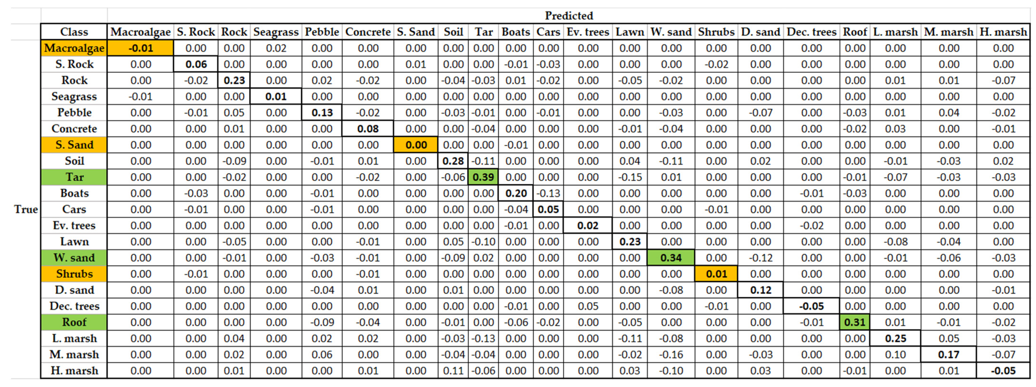
Classification performances were assessed by considering the values obtained on the test dataset by the random forest classifier for the following metrics: overall accuracy (OA, ratio of correct predictions, best when its value is 1), precision (fraction of correct predictions among each ground truth classes, best when its value is 1), recall (fraction of correct estimation for each predicted classes, best when its value is 1), and F-score (combination of precision and recall, best when its value is 1). The precision, recall, and F-score were computed for each label, and their unweighted mean was used to compare the results obtained. Confusion matrixes presenting the producer’s accuracies (PA) were also created to analyze the performances of classification on each of the 21 classes.

3.9. Spatialization of the Random Forest Predictions

Although coordinates were not used during classification, the arrays of features were geolocated with the position of the waveform’s last echo, as illustrated by Figure 5. To visualize our classification results as PCs, we associated the predictions’ vector to these coordinates. This allowed us to obtain the result under the form of a classified PC. The fact that we did not rasterize our data had the advantage of preserving the spatial density and therefore the spatial resolution, while also avoiding the critical issue of mixed pixels [46].
Each waveform was localized with the planar coordinates of its last return using the PC coordinates. For bathymetric waveforms, this ensured that the effects of refraction of the laser beam on the air/water interface were considered, since the green PC was corrected before data delivery.

4. Results

4.1. Random Forest Classifications’ Performances on the Test Dataset

Ten random forest models were trained on the training dataset—one for each configuration of predictors defined in Section 3.7. Their performances were evaluated using four metrics computed on the predictions made on the test dataset. Four of them were then used to predict labels for the complete study area and produce habitat maps under the form of PCs.
Fitting the models to the 21,000 items training dataset took on average 0.4 s. Predictions on the test dataset (which contains 10,500 items) required a mean computing time of 0.2 s. The complete area, representing a total of more than 24.5 million items, was covered in 17 to 18 min. All computations were made on a machine equipped with an AMD Ryzen 9 5900X 12-Core CPU and an NVIDIA GeForce RTX 3080 GPU.
The classification metrics obtained on each set of features defined in Section 3.7. are presented in Table 3. The very close values observed between the four criteria for each feature set are due to the averaging of each metric’s value obtained for each classification label. They are also explained by the fact that all classes are balanced. The scores obtained show that our method does not have a systematic tendency to over- or under-estimate some classes.
When using only subsets of green waveform features, the random forest predictions were more often false than they were correct. However, grouping the waveform variable families improved the accuracy by at least 4%. The best configuration—composed of peak shape features and lidar return features—provided a classification accuracy of 69%. Globally, coupling statistical features with peak shapes features tended to result in accuracy loss while using combinations where they were not mixed resulted in classification performance gains. Indeed, the complete set of features obtained through green waveform processing predicted the habitat type with an OA of 56%, while the output of the classification of statistical and lidar return features was correct in 67% of cases (see Table 3).
The addition of IR intensity values to the full set of green waveform parameters improved the OA of 13%, which is 5% above the best OA obtained on a subset of green waveform attributes. The contribution of the elevation to the classification accuracy was even higher: there was a 31.5% gain in OA between the green spectral features’ classification and the classification of green spectral features and elevations. Gathering the three sources of information produced the most accurate result, with an OA of 90.5% (Table 3).

4.2. Green Waveform Features’ Contribution to the Classification Accuracy

Figure 8 illustrates the contribution of each predictor to the accuracy of the classification of green waveform features. It sheds light on the value-added of each attribute computed on the truncated waveforms. This assessment reveals that 9 of the 16 features extracted on each waveform contributed positively to the classification performance. The seven others had a negative impact on the quality of the random forest predictions. They were mostly parameters of the “statistical features” set, although each type of waveform parameter—statistical, peak shape-related, or lidar return-related—was represented in the nine positively contributing attributes.
An in-depth analysis of the four last random forest experiments is provided in the following sections.

4.3. Land-Water Continuum Habitat 3D Modelling

By running the waveform processing algorithm and the classifiers on the whole study area, we obtained a 21-class semantic segmentation of our complete bathymetric lidar dataset.
As expected, when dealing with PCs and not rasters, the results were noisy, but some areas had lower speckle than others. The observable ratio between information and noise gradually improved with the addition of IR intensity and elevations. The best output was obtained by combining green waveform features, IR intensities, and elevations; it is presented in Figure 9. The other results are presented in Appendix A (Figure A1, Figure A2 and Figure A3).
The main strength of this result was the distinction between submerged and emerged domains: except for boat false-positives on the water surface, marine classes were rarely detected over land, and vice versa. Globally, this map showed better definition of the considered habitats than the others (see Figure A1, Figure A2 and Figure A3), and fewer classification errors, although improvements on some classes coexisted with poorer performance on other classes. Figure 10, Figure 11, Figure 12 and Figure 13 gave a more detailed insight into the classification in specific areas.

4.3.1. Urban Area and Sand Beach Classification

As Figure 10 shows, the detection of planar, highly reflective surfaces such as tar and concrete was accurate, but their specific type was sometimes misidentified. Although the pier located north of Figure 10 was correctly mapped as concrete, there was confusion between soil and tar on the sandy dune (southeast of the same figure).
The classification of roof was satisfactory both west and east of the area presented in Figure 10 but showed cases of overdetection. In the urban area developed on the sandy dune (southeast of Figure 10), tar, rooves, trees, and shrubs were distinguished precisely, but sandy dune vegetation, shrubs, and trees were sometimes confused for rooves or tar.
A weaker aspect of this result was the classification of the sand beaches: patches of wet sand were well defined, but the borders between wet and dry sand featured many false detections of pebble. Confusion between pebble and sand was high, as shown in the wide area of sand beach that is classified as pebble in the northeast in Figure 10.

4.3.2. Salt Marsh Classification

Figure 11 presented a closer look at the classification obtained in the salt marsh area. The three types of salt marsh distinguished—low, mid, and high marsh—appeared to be well identified.
The classification of the salt marsh channels was less correct: instead of wet sand and submerged sand, the classifier predicted rock and submerged rock in various areas.

4.3.3. Seagrass Meadow Classification

In Figure 12, the focus was set on the seagrass meadow located in the north of the study site. Emerged and submerged parts of the rocky island were well mapped, even though submerged rock was detected in places where the seabed is sandy. The two types of underwater vegetation we attempted to map were very precisely defined: the patches of seagrass meadow and macroalgae were mapped with very low confusion with submerged sand or rock. However, the type of underwater vegetation (macroalgae or seagrass) was not correct in all places. There were classification errors in the seagrass meadow, where macroalgae was detected. Seagrasses were also found in macroalgae-covered areas.
Figure 12 also showed the precision of the classification of boats: boats mooring in the seagrass meadow were correctly labelled even though no training or test data were collected in that area for the boats class.

4.4. Confusion Matrix Obtained with Green Waveform Features, Infrared Intensities and Elevations on the Test Dataset

The confusion matrix obtained using green waveform features, IR intensities, and elevations on the test dataset is presented in Figure 13. It confirmed the observations made on the visual results. All classes were predicted with at least 70% of correctness. The most frequent confusions were between seagrasses and macroalgae, deciduous and evergreen trees, and submerged rock and submerged sand, which corroborated the observations made on the application of the model to the broader dataset.
The other confusion matrixes can be found in Appendix B (Figure A4, Figure A5 and Figure A6).

5. Discussion

We improved an approach initially designed to distinguish two seabed covers—fine sediment and seagrass—to map all land and sea covers present in our study scene in 3D. The findings showed lidar waveforms can be used to classify and map habitats of the coastal fringe and bridge the gap between marine and terrestrial surveys. All 21 selected classes were classified with at least 70% of accuracy in the best configuration obtained, which had an OA of 90%. Here, we discuss the results obtained regarding the classification predictors and the methodology employed. We also provide potential explanations for the performances of the algorithm.

5.1. Green Waveform Features

Our research partially aimed at exploring whether green lidar waveforms can be relevant for coastal habitat mapping. We defined 16 features to extract from the portions of the waveforms that correspond to layers of ground or seabed covers. These were efficiently retrieved both on land and underwater. However, our approach did not handle extremely shallow waters, where the surface component and the bottom return overlap in the waveforms. In these cases, the peak detection employed did not distinguish the seabed from the water surface and no features were retrieved. There was consequently a 24 m wide band without data in the surf zone on the sand beaches in our processed lidar dataset. We also noticed cases of confusion between seabed return and noise in the water column component of the waveform, which resulted in a mis-located detected seabed. These issues could be handled by improving the way the different waveform components are isolated: using waveform decomposition [31] or deconvolution [47,48] could produce better results on that aspect.
The features defined to describe the spectral signatures of coastal habitats seemed to be equally relevant for land and sea covers mapping. However, they did not provide a highly accurate classification (56% of OA). This can be explained by analyzing the green waveforms obtained with the HawkEye III on land. Since this sensor was particularly designed for bathymetry extraction, its green lasers are set to be powerful enough to reach the seabed up to several dozens of meters in coastal waters. Over land, the laser power is so high that most of the waveforms originating from highly reflective surfaces are saturated. The green wavelength alone might consequently not encompass a fine enough range of intensities over land to allow separation of similar environments such as plane habitats, different types of herbaceous vegetation, etc. The shapes of the saturated waveform returns are also affected: there is lacking information on the shape of the peak around its maximum. This can explain why there was a lot of confusion between topographic habitats when using green waveforms only.
Though green information alone may not be enough to distinguish the 21 habitats accurately, our findings suggested that a finer selection of the waveform attributes used for classification could enhance the green waveform feature predictions. The results presented in Table 3 and Figure 8 revealed negative interactions between some of the features chosen. Combining the full sets of statistical and peak shape features (defined in Section 3.7) resulted in lower accuracy than using them separately. Furthermore, the predictors’ contribution assessment (Figure 8) showed that out of the 16 predictors, only nine contributed positively to the classification accuracy. This might be due to information redundancy between features relying on similar concepts such as mean and median intensity, for example. It could be due to the correction of attenuation performed on bathymetric waveforms. This exponential correction produced extremely high values of backscattered intensities under water, which made little sense physically. On the other hand, topographic waveforms were not corrected: their typical intensity order of magnitude was several times smaller, which might have disrupted the classifier. Fixing the issue of attenuation correction and using only a selected set of waveform predictors based on an assessment of their contribution would certainly result in better results when using the green wavelength alone.
The three different types of waveform features appeared to be complimentary: the nine predictors with a positive influence on the OA (Figure 8) represented each feature family defined in Section 3.7. This was consistent: the shape of the waveform return is characteristic of its nature, and the complexity, length, shape, maximum, and position of its maximum sum up the essential information differentiating one waveform from another.

5.2. Infrared Data

The addition of the IR wavelength increased the OA by 13%. The classification results certainly benefited from IR light’s interaction with water and chlorophyll pigments, which provided essential information for the labelling of vegetation and other topographic classes such as wet sand. Considering that the green wavelength was less adapted to land cover classification, the performance increase obtained by using both lasers was expected.
Our research showed the added value of topobathymetric lidar: on top of providing quasi-continuity between land and water, both wavelengths provided complementary information for land covers’ classification. The IR PC alone could not provide a coastal habitat map since it did not reach the seabed and riverbed; the OA obtained using only this wavelength (24%, presented in Table 3) confirmed that. They also showed that green lidar features alone do not provide a sufficient basis for classification either, reaching an OA of only 56%. Coupling both wavelengths improved the overall result significantly, bringing together the strengths of IR data on land covers, and the ability of green lidar to penetrate the water surface. The matrixes presented in Figure A4 and Figure A5 show that the addition of IR intensities to green waveform features resulted in an accuracy increase for all but two of the 21 classes. The gain ranged between 0% (submerged sand) and 39% (tar). The minimum accuracy observed over the 21 labels rose from 21% to 29%. Water covers classes such as seagrass and submerged rock also benefited from the addition of IR intensities, as their accuracy showed an improvement of 1% and 6%, respectively. As HawkEye III is tailored for bathymetry, its green laser’s power was set to be high, which resulted in saturated intensities over land. The IR channel provided complimentary information in places when the green channel was weaker, which partially explains the algorithm’s performances we observe. The classification accuracies obtained for land covers confirm that; for example, the classification of soil, wet sand, and lawn was significatively enhanced: +28%, +34%, and +23% of OA, respectively. Our future work will focus on exploiting both IR and green waveforms for habitat classification, to maximize the accuracy attainable with full-waveform topobathymetric lidar.

5.3. Ground and Seabed Elevation

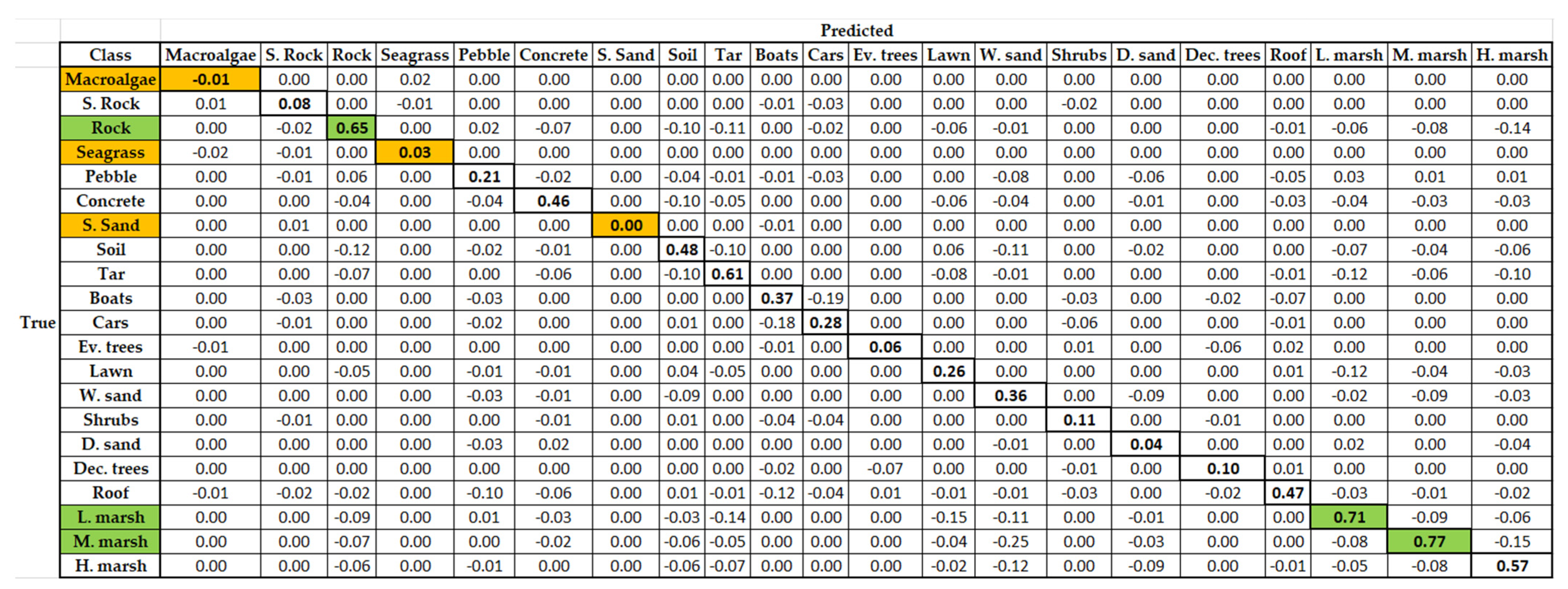
Similarly to the IR data, elevations contributed greatly to the improvement of the OA of the habitat classification, but could not be separated from spectral predictors and used alone to provide accurate detection of land and sea covers. Indeed, Table 3 revealed that elevations produced a classification with an OA of 55%, which is less than what can be achieved with spectral predictors. This was expected since many different habitats coexist at similar altitudes and are mainly differentiated by their reflectance. However, for some others, mainly salt marsh types, elevation is an intrinsic quality and the base of their definition. This explains why those are the type of classes that benefited the most from the addition of elevation to a set of spectral predictors in terms of classification accuracy. Respectively, the classification accuracy of low salt marsh, mid salt marsh, and high salt marsh rose from 71%, 76%, and 21% by adding elevations to the green waveform features in the set of predictors (see Figure A4 and Figure A6).
Even though elevation combined with spectral information already provided high classification accuracy (90%, see Table 3), the values extracted with our approach were not always consistent with those provided by the original PCs in marine areas, as explained above. To remove artifacts due to water quality, a post-processing step could be implemented, and the neighboring elevations could be used to regularize the processed PC obtained.

5.4. Classification Approach

Our results showed that topobathymetric lidar is fitted to the classification of coastal habitats. Although elevations, IR intensities, and green waveform features did not produce high accuracy classifications of the land-water continuum, they were complimentary and achieved high-precision results when combined. To the best of our knowledge, no similar papers proposing point-based land and water covers mapping from bispectral lidar data were published, so no direct comparisons of results are possible. However, our observations corroborate those made in [35], which successfully used random forest algorithms to classify full-waveform lidar data over urban areas and obtained an overall accuracy of over 94% when identifying four types of land covers. This paper only focuses on terrestrial areas but confirms the high accuracy we observe when using waveform features without rasterization for mapping purposes. Class-wise, our results seem more homogeneous for the land covers we have in common, although this means that our approach performs less accurately than theirs on some urban classes. Indeed, ref. [35] presents a PA of 94.8% for buildings, which is higher than we observe on our roof class (89%), but our vegetation classes (trees and shrubs) have an average PA of 82.6%, while theirs is 68.9%, and our natural ground classes (soil, lawn, salt marsh) reach an average PA of 91.6%, higher than the 32.7% presented in [35]. Our approach and the method introduced in [35] perform similarly on artificial ground (for us, tar and concrete), with PAs of 96% and 96.4%, respectively.
Although we found no other research performing point-based classification of subtidal, intertidal, and supra-tidal habitats, we can compare our findings to those in [34], where the authors also observed that the use of waveform data improves seabed maps and obtained an OA of 86% for their classification of seabed substrates and aquatic macrovegetation. Their approach provides a better mapping of low underwater vegetation on soft substrate (100% versus 85% of PA in our case) but a less accurate detection of hard seabed substrate (68% versus 90% of PA in our study). Again, although we have less accurate results for some classes, our method seems to provide more balanced and homogeneous performances among different classes.
Our results also confirm those from [27], where 19 land-water continuum habitats were classified with an OA of 90%, and in which the authors concluded that the best classification results were obtained when combining spectral information and elevation. However, in [27], the authors used digital models of waveform features that they obtained by rasterizing their data, and they relied on an ML classifier. Although our metrics are similar, our classification has the advantage of preserving the spatial density and repartition of the data.
Other studies such as [49,50,51] used 2D lidar-derived data and imagery along with machine learning classifiers to map similar coastal habitats as the ones we attempted to map. They obtained performance scores in the same range as ours, with OA between 84% and 92%. The authors did not use waveform data in these studies and observed low accuracy when classifying only digital elevation models obtained with lidar surveys, therefore requiring the additional processing of imagery. Our approach has the advantage of requiring only one source of data out of the two sources often used in existing literature, which facilitates both acquisition procedures and processing.
Globally, our results are in line with [27,35,52], which all state that bathymetric lidar waveforms are well suited for benthic habitats mapping and observe the same complementarity between spectral and elevation information for habitat mapping. Our method offers an OA similar to existing research in lidar data classification for habitat mapping, while extending the application to a wider range of habitats—both marine and terrestrial—and avoiding information loss through rasterization. Although the PAs obtained for some classes are lower than results previously presented in other studies [34,35], this method also has the advantage of offering homogeneous performances and low inter classes PA differences, contrary to other existing research results [34,35].
The random forest models trained showed low overfitting, as the extended application results illustrated. The classification of boats located outside of the training and test data collection area, for example, illustrated that the classifiers obtained could be applied to other datasets accurately. Natural, semi-natural and anthropic habitats were well distinguished, and vegetation was precisely isolated, which opened perspectives for ecological assessments of those coastal areas. The remaining errors often involved classes that were close semantically. For example, there was confusion between salt marsh and high natural grasses but low confusion between lawns and low marsh. A potential improvement could be to review the classes defined initially and distinguish vegetation by layers (herbaceous, arbustive, arborescent) and by their natural, semi-natural, or anthropic nature.
Besides the quality of the training and test datasets established, a source of explanation for remaining classification errors could be found in the technical specifications of the sensor. The diameter of the HawkEye III’s green laser’s footprint is 1.80 m, which means that the returned waveform condensates information in a 2.5 m2 area. This parameter may have had an influence on the ability of a given array of features to describe pebble or sand, mostly at interfaces between habitats. This could partially explain the confusion between deciduous and evergreen trees: in a mixed-species forest, two different trees can coexist in a 2.5 m2 patch.
Although the main issues identified visually reflected in the metrics computed on the test dataset, there was a gap between the estimated quality of the map and the statistics computed. For example, the classification of portions of sandy beaches as pebble was not as obvious in the confusion matrix as it is in the map. This showed the influence of the way the test dataset is built. Further work should try to incorporate validation maps in addition to test datasets to qualify the output on the complete study site. A finer tree species inventory could also be integrated to better assess the results obtained.
Nonetheless, our results highlighted a strong classification approach, leveraging the strengths of 3D bispectral data. Working at the PC scale and not in 2D opens perspectives for 3D classifications, identifying all layers of land and sea cover, mostly in vegetated areas, by using waveform segmentation instead of waveform PC segmentation, as experimented in [53]. It also shows possibilities for post-processing and neighbor-based result regularization, as well as the exploitation of spatial information through the addition of geometrical features such as roughness or local density. Lastly, the accurate classification of habitats through 3D data offers opportunities for structural ecology assessments and communication of these results to environmental managers through virtual reality or more relatable 3D visualizations, for the implementation of sustainable integrated management of coastal areas. Figure 14 provides a 3D view of the 3D habitat mapping achieved in the present study.

6. Conclusions

In this article, we proposed an approach to map coastal habitats exclusively using topobathymetric lidar, including both full waveforms and reanalyzed echoes. We produced results under the form of PCs and extended the application of our best classifier—which obtained 90% of OA on the test dataset—to a dataset of 24.5 million points covering a very diverse coastal area. A total of 21 classes of land and sea covers were defined and mapped in 3D. We found that green waveforms and IR intensities complement each other: while green data provided strong results in submerged areas, the IR wavelength improved the distinction of land covers. Elevations further increased the classification accuracy by perfecting the classification of plane classes and classes, such as low, mid, and high salt marsh, which were principally differentiated by their elevation. It is of special interest to note that green waveforms alone produced better results than IR intensities or elevations alone. However, the combination of the three sources of information yielded the best result, highlighting that they each bring a specific contribution to the result. Our research showed how fit topobathymetric lidar is to the classification of such numerous land-water interface habitats. We enhanced a waveform processing method to apply it to topo-bathymetric environments. The use of PCs instead of rasters and the addition of a second wavelength provided an original 3D map of 21 coastal habitats at very high spatial resolution. This provides encouraging perspectives for 3D mapping and ecological assessment of the land-water interface and paves the way to integrated management of coastal areas, bridging the gap between marine and terrestrial domains.

Author Contributions

Conceptualization, M.L., A.C., T.C. and D.L.; methodology, M.L.; software, M.L.; validation, M.L.; formal analysis, M.L.; investigation, M.L.; resources, Y.P., A.E., A.C. and M.L.; data curation, M.L. and Y.P.; writing—original draft preparation, M.L.; writing—review and editing, M.L., A.C., T.C., D.L., Y.P. and A.E.; visualization, M.L.; supervision, A.C., T.C. and D.L.; project administration, A.C., T.C. and D.L.; funding acquisition, M.L., A.C., T.C. and D.L. All authors have read and agreed to the published version of the manuscript.

Funding

This research was funded by a Ph.D. grant from Région Bretagne, and by the Saur Group’s patronage. The APC was funded by the Nantes-Rennes topobathymetric lidar platform of the University of Rennes 1.

Data Availability Statement

Data sharing is not applicable to this article.

Acknowledgments

The authors are grateful to Airborne Hydrography AB (AHAB), an affiliate company of Leica Geosystems, for their technical support, their assistance with software and development issues, and their help in understanding the specificities of the sensor and its data. M.L. would like to thank the lab members who contributed to ground truth data acquisition—Hélène Gloria, Dorothée James, Alyson Le Quilleuc, Antoine Mury, and Léna Véle—and external volunteers. M.L. is also grateful to the Rennes 2 University for the field work equipment support. The authors deeply acknowledge the input of the anonymous reviewers, which improved the quality of the manuscript.

Conflicts of Interest

The authors declare no conflict of interest. The funders had no role in the design of the study; in the collection, analyses, or interpretation of data; in the writing of the manuscript, or in the decision to publish the results.

Appendix A

Appendix A contains the projected 3D maps of the habitats obtained for 3 random forest experiments: the classification of green waveform features only, the classification of green waveform features and IR intensities, and the classification of green waveform features and elevations.
Figure A1. Projected 3D map of the habitats obtained with the predictions of a random forest classifier on green spectral features; orthoimage of the study area. The orthoimage was captured in 2014, while lidar data are not contemporaneous as they date from 2019. S. = submerged, Ev. = evergreen, Dec. = deciduous.
Remotesensing 14 00341 g0a1
Figure A2. Projected 3D map of the habitats obtained with the predictions of a random forest classifier on green spectral features and infrared intensities; orthoimage of the study area. The orthoimage was captured in 2014, while lidar data are not contemporaneous as they date from 2019. S. = submerged, Ev. = evergreen, Dec. = deciduous.
Remotesensing 14 00341 g0a2
Figure A3. Projected 3D map of the habitats obtained with the predictions of a random forest classifier on green spectral features and elevation values; orthoimage of the study area. The orthoimage was captured in 2014, while lidar data are not contemporaneous as they date from 2019. S. = submerged, Ev. = evergreen, Dec. = deciduous.
Remotesensing 14 00341 g0a3

Appendix B

Appendix B contains the confusion matrix or difference matrixes obtained for 3 random forest experiments: the classification of green waveform features only, the classification of green waveform features and IR intensities, and the classification of green waveform features and elevations.
Figure A4. Confusion matrix obtained by the random forest classification of the green waveforms’ features. The three highest and three lowest class accuracy values are highlighted in green and orange, respectively. S. = submerged, Ev. = evergreen, Dec. = deciduous.
Remotesensing 14 00341 g0a4
Figure A5. Difference of the confusion matrixes obtained for the classification of green waveforms’ features plus infrared intensities, and green waveforms’ features only. The three highest and three lowest class accuracy values are highlighted in green and orange, respectively. S. = submerged, Ev. = evergreen, Dec. = deciduous.
Remotesensing 14 00341 g0a5
Figure A6. Difference of the confusion matrixes obtained for the classification of green waveforms’ features plus elevations, and green waveforms’ features only. The three highest and three lowest values are highlighted in green and orange, respectively. S. = submerged, Ev. = evergreen, Dec. = deciduous.
Remotesensing 14 00341 g0a6

References

  1. Barbier, E.B.; Hacker, S.D.; Kennedy, C.; Koch, E.W.; Stier, A.C.; Silliman, B.R. The Value of Estuarine and Coastal Ecosystem Services. Ecol. Monogr. 2011, 81, 169–193. [Google Scholar] [CrossRef]
  2. Turner, R.K.; Schaafsma, M.; Mee, L.; Elliott, M.; Burdon, D.; Atkins, J.P.; Jickells, T. Conceptual Framework. In Coastal Zones Ecosystem Services: From Science to Values and Decision Making; Turner, R.K., Schaafsma, M., Eds.; Studies in Ecological Economics; Springer International Publishing: Cham, Switzerland, 2015; pp. 11–40. ISBN 978-3-319-17214-9. [Google Scholar]
  3. Mury, A.; Collin, A.; Etienne, S.; Jeanson, M. Wave Attenuation Service by Intertidal Coastal Ecogeosystems in the Bay of Mont-Saint-Michel, France: Review and Meta-Analysis. In Proceedings of the 20th EGU General Assembly EGU2018, Vienna, Austria, 4–13 April 2018; pp. 555–572. [Google Scholar]
  4. Collin, A.; Dubois, S.; James, D.; Houet, T. Improving Intertidal Reef Mapping Using UAV Surface, Red Edge, and Near-Infrared Data. Drones 2019, 3, 67. [Google Scholar] [CrossRef] [Green Version]
  5. Collin, A.; Dubois, S.; Ramambason, C.; Etienne, S. Very High-Resolution Mapping of Emerging Biogenic Reefs Using Airborne Optical Imagery and Neural Network: The Honeycomb Worm (Sabellaria Alveolata) Case Study. Int. J. Remote Sens. 2018, 39, 5660–5675. [Google Scholar] [CrossRef] [Green Version]
  6. Collin, A.; Lambert, N.; Etienne, S. Satellite-Based Salt Marsh Elevation, Vegetation Height, and Species Composition Mapping Using the Superspectral WorldView-3 Imagery. Int. J. Remote Sens. 2018, 39, 5619–5637. [Google Scholar] [CrossRef]
  7. Kutser, T.; Hedley, J.; Giardino, C.; Roelfsema, C.; Brando, V.E. Remote Sensing of Shallow Waters—A 50 Year Retrospective and Future Directions. Remote Sens. Environ. 2020, 240, 111619. [Google Scholar] [CrossRef]
  8. Collin, A.; Etienne, S.; Feunteun, E. VHR Coastal Bathymetry Using WorldView-3: Colour versus Learner. Remote Sens. Lett. 2017, 8, 1072–1081. [Google Scholar] [CrossRef]
  9. Collin, A.; Hench, J.L.; Pastol, Y.; Planes, S.; Thiault, L.; Schmitt, R.J.; Holbrook, S.J.; Davies, N.; Troyer, M. High Resolution Topobathymetry Using a Pleiades-1 Triplet: Moorea Island in 3D. Remote Sens. Environ. 2018, 208, 109–119. [Google Scholar] [CrossRef]
  10. Adler-Golden, S.M.; Acharya, P.K.; Berk, A.; Matthew, M.W.; Gorodetzky, D. Remote Bathymetry of the Littoral Zone from AVIRIS, LASH, and QuickBird Imagery. IEEE Trans. Geosci. Remote Sens. 2005, 43, 337–347. [Google Scholar] [CrossRef]
  11. Collin, A.; Andel, M.; Lecchini, D.; Claudet, J. Mapping Sub-Metre 3D Land-Sea Coral Reefscapes Using Superspectral WorldView-3 Satellite Stereoimagery. Oceans 2021, 2, 315–329. [Google Scholar] [CrossRef]
  12. Stumpf, R.P.; Holderied, K.; Sinclair, M. Determination of Water Depth with High-Resolution Satellite Imagery over Variable Bottom Types. Limnol. Oceanogr. 2003, 48, 547–556. [Google Scholar] [CrossRef]
  13. Lesser, M.; Mobley, C. Bathymetry, Water Optical Properties, and Benthic Classification of Coral Reefs Using Hyperspectral Remote Sensing Imagery. Coral Reefs 2007, 26, 819–829. [Google Scholar] [CrossRef]
  14. Klonowski, W.M.; Fearns, P.R.C.S.; Lynch, M.J. Retrieving Key Benthic Cover Types and Bathymetry from Hyperspectral Imagery. J. Appl. Remote Sens. 2007, 1, 011505. [Google Scholar] [CrossRef]
  15. Sandidge, J.C.; Holyer, R.J. Coastal Bathymetry from Hyperspectral Observations of Water Radiance. Remote Sens. Environ. 1998, 65, 341–352. [Google Scholar] [CrossRef]
  16. Kutser, T.; Vahtmäe, E.; Martin, G. Assessing Suitability of Multispectral Satellites for Mapping Benthic Macroalgal Cover in Turbid Coastal Waters by Means of Model Simulations. Estuar. Coast. Shelf Sci. 2006, 67, 521–529. [Google Scholar] [CrossRef]
  17. Wedding, L.M.; Friedlander, A.M.; McGranaghan, M.; Yost, R.S.; Monaco, M.E. Using Bathymetric Lidar to Define Nearshore Benthic Habitat Complexity: Implications for Management of Reef Fish Assemblages in Hawaii. Remote Sens. Environ. 2008, 112, 4159–4165. [Google Scholar] [CrossRef]
  18. Nie, S.; Wang, C.; Zeng, H.; Xi, X.; Li, G. Above-Ground Biomass Estimation Using Airborne Discrete-Return and Full-Waveform LiDAR Data in a Coniferous Forest. Ecol. Indic. 2017, 78, 221–228. [Google Scholar] [CrossRef]
  19. Ene, L.T.; Næsset, E.; Gobakken, T.; Gregoire, T.G.; Ståhl, G.; Nelson, R. Assessing the Accuracy of Regional LiDAR-Based Biomass Estimation Using a Simulation Approach. Remote Sens. Environ. 2012, 123, 579–592. [Google Scholar] [CrossRef]
  20. Lindberg, E.; Olofsson, K.; Holmgren, J.; Olsson, H. Estimation of 3D Vegetation Structure from Waveform and Discrete Return Airborne Laser Scanning Data. Remote Sens. Environ. 2012, 118, 151–161. [Google Scholar] [CrossRef] [Green Version]
  21. Guenther, G.C. Airborne Laser Hydrography: System Design and Performance Factors; National Oceanic and Atmospheric Administration: Rockville, MD, USA, 1985; pp. 23–40. [Google Scholar]
  22. Philpot, W. Airborne Laser Hydrography II. Available online: https://ecommons.cornell.edu/handle/1813/66666 (accessed on 30 October 2021).
  23. Brodu, N.; Lague, D. 3D Terrestrial Lidar Data Classification of Complex Natural Scenes Using a Multi-Scale Dimensionality Criterion: Applications in Geomorphology. ISPRS J. Photogramm. Remote Sens. 2012, 68, 121–134. [Google Scholar] [CrossRef] [Green Version]
  24. Hansen, S.S.; Ernstsen, V.B.; Andersen, M.S.; Al-Hamdani, Z.; Baran, R.; Niederwieser, M.; Steinbacher, F.; Kroon, A. Classification of Boulders in Coastal Environments Using Random Forest Machine Learning on Topo-Bathymetric LiDAR Data. Remote Sens. 2021, 13, 4101. [Google Scholar] [CrossRef]
  25. Teo, T.-A.; Wu, H.-M. Analysis of Land Cover Classification Using Multi-Wavelength LiDAR System. Appl. Sci. 2017, 7, 663. [Google Scholar] [CrossRef] [Green Version]
  26. Guo, Y.; Wang, H.; Hu, Q.; Liu, H.; Liu, L.; Bennamoun, M. Deep Learning for 3D Point Clouds: A Survey. IEEE Trans. Pattern Anal. Mach. Intell. 2021, 43, 4338–4364. [Google Scholar] [CrossRef]
  27. Collin, A.; Long, B.; Archambault, P. Merging Land-Marine Realms: Spatial Patterns of Seamless Coastal Habitats Using a Multispectral LiDAR. Remote Sens. Environ. 2012, 123, 390–399. [Google Scholar] [CrossRef]
  28. Mallet, C.; Bretar, F. Full-waveform topographic lidar: State-of-the-art. ISPRS J. Photogramm. Remote Sens. 2009, 64, 1–16. [Google Scholar] [CrossRef]
  29. Letard, M.; Collin, A.; Lague, D.; Corpetti, T.; Pastol, Y.; Ekelund, A.; Pergent, G.; Costa, S. Towards 3D Mapping of Seagrass Meadows with Topo-Bathymetric Lidar Full Waveform Processing. In Proceedings of the 2021 IEEE International Geoscience and Remote Sensing Symposium IGARSS, Brussels, Belgium, 11–16 July 2021; pp. 8069–8072. [Google Scholar]
  30. Song, S.; Wang, B.; Gong, W.; Chen, Z.; Xin, L.; Sun, J.; Shi, S. A New Waveform Decomposition Method for Multispectral LiDAR. ISPRS J. Photogramm. Remote Sens. 2019, 149, 40–49. [Google Scholar] [CrossRef]
  31. Shen, X.; Li, Q.-Q.; Wu, G.; Zhu, J. Decomposition of LiDAR Waveforms by B-Spline-Based Modeling. ISPRS J. Photogramm. Remote Sens. 2017, 128, 182–191. [Google Scholar] [CrossRef]
  32. Chauve, A.; Mallet, C.; Bretar, F.; Durrieu, S.; Deseilligny, M.P.; Puech, W. Processing full-waveform lidar data: Modelling raw signals. In Proceedings of the ISPRS Workshop on Laser Scanning 2007, Espoo, Finland, 12 September 2007; Volume 36, pp. 102–107. [Google Scholar]
  33. Eren, F.; Pe’eri, S.; Rzhanov, Y.; Ward, L. Bottom Characterization by Using Airborne Lidar Bathymetry (ALB) Waveform Features Obtained from Bottom Return Residual Analysis. Remote Sens. Environ. 2018, 206, 260–274. [Google Scholar] [CrossRef]
  34. Tulldahl, H.M.; Wikström, S.A. Classification of Aquatic Macrovegetation and Substrates with Airborne Lidar. Remote Sens. Environ. 2012, 121, 347–357. [Google Scholar] [CrossRef]
  35. Chehata, N.; Guo, L.; Mallet, C. Airborne lidar feature selection for urban classification using random forests. In Proceedings of the Laserscanning, Paris, France, 1–2 September 2009. [Google Scholar]
  36. Yan, W.Y.; Shaker, A.; El-Ashmawy, N. Urban Land Cover Classification Using Airborne LiDAR Data: A Review. Remote Sens. Environ. 2015, 158, 295–310. [Google Scholar] [CrossRef]
  37. Niemeyer, J.; Wegner, J.D.; Mallet, C.; Rottensteiner, F.; Soergel, U. Conditional Random Fields for Urban Scene Classification with Full Waveform LiDAR Data. In Proceedings of the Photogrammetric Image Analysis; Stilla, U., Rottensteiner, F., Mayer, H., Jutzi, B., Butenuth, M., Eds.; Springer: Berlin/Heidelberg, Germany, 2011; pp. 233–244. [Google Scholar]
  38. Pastol, Y. Use of Airborne LIDAR Bathymetry for Coastal Hydrographic Surveying: The French Experience. J. Coast. Res. 2011, 62, 6–18. [Google Scholar] [CrossRef]
  39. Lague, D.; Feldmann, B. Chapter 2—Topo-bathymetric airborne LiDAR for fluvial-geomorphology analysis. In Developments in Earth Surface Processes; Tarolli, P., Mudd, S.M., Eds.; Remote Sensing of Geomorphology; Elsevier: Amsterdam, The Netherlands, 2020; Volume 23, pp. 25–54. [Google Scholar]
  40. Kashani, A.G.; Olsen, M.J.; Parrish, C.E.; Wilson, N. A Review of LIDAR Radiometric Processing: From Ad Hoc Intensity Correction to Rigorous Radiometric Calibration. Sensors 2015, 15, 28099–28128. [Google Scholar] [CrossRef] [Green Version]
  41. Wilson, N.; Parrish, C.E.; Battista, T.; Wright, C.W.; Costa, B.; Slocum, R.K.; Dijkstra, J.A.; Tyler, M.T. Mapping Seafloor Relative Reflectance and Assessing Coral Reef Morphology with EAARL-B Topobathymetric Lidar Waveforms. Estuaries Coasts 2019. [Google Scholar] [CrossRef] [Green Version]
  42. Shom, IGN, Etat Français, Région Bretagne, DREAL Bretagne, FEDER. Litto3D® Bretagne. 2021. Available online: https://diffusion.shom.fr/pro/risques/altimetrie-littorale.html (accessed on 30 October 2021).
  43. Girardeau-Montaut, D. CloudCompare. 2016. Available online: https://www.danielgm.net/cc/ (accessed on 30 October 2021).
  44. Collin, A.; Long, B. Mapping the Shallow Water Seabed Habitat with the Shoals. IEEE Trans. Geosci. Remote Sens. 2008, 46, 2947–2955. [Google Scholar] [CrossRef]
  45. Oshiro, T.M.; Perez, P.S.; Baranauskas, J.A. How Many Trees in a Random Forest? In Proceedings of the Machine Learning and Data Mining in Pattern Recognition; Perner, P., Ed.; Springer: Berlin/Heidelberg, Germany, 2012; pp. 154–168. [Google Scholar]
  46. Hsieh, P.-F.; Lee, L.C.; Chen, N.-Y. Effect of Spatial Resolution on Classification Errors of Pure and Mixed Pixels in Remote Sensing. IEEE Trans. Geosci. Remote Sens. 2001, 39, 2657–2663. [Google Scholar] [CrossRef]
  47. Zhou, T.; Popescu, S.C.; Krause, K.; Sheridan, R.D.; Putman, E. Gold—A Novel Deconvolution Algorithm with Optimization for Waveform LiDAR Processing. ISPRS J. Photogramm. Remote Sens. 2017, 129, 131–150. [Google Scholar] [CrossRef]
  48. Wu, J.; van Aardt, J.A.N.; Asner, G.P. A Comparison of Signal Deconvolution Algorithms Based on Small-Footprint LiDAR Waveform Simulation. IEEE Trans. Geosci. Remote Sens. 2011, 49, 2402–2414. [Google Scholar] [CrossRef]
  49. Butler, J.D.; Purkis, S.J.; Yousif, R.; Al-Shaikh, I.; Warren, C. A High-Resolution Remotely Sensed Benthic Habitat Map of the Qatari Coastal Zone. Mar. Pollut. Bull. 2020, 160, 111634. [Google Scholar] [CrossRef]
  50. Grande, M.; Chust, G.; Fernandes, J.; Galparsoro Iza, I. Assessment of the Discrimination Potential of Bathymetric LIDAR and Multispectral Imagery for Intertidal and Subtidal Habitats. In Proceedings of the 33th International Symposium on Remote Sensing of Environment (ISRSE), Stresa, Italy, 12 February 2009. [Google Scholar]
  51. Chust, G.; Grande, M.; Galparsoro, I.; Uriarte, A.; Borja, Á. Capabilities of the Bathymetric Hawk Eye LiDAR for Coastal Habitat Mapping: A Case Study within a Basque Estuary. Estuar. Coast. Shelf Sci. 2010, 89, 200–213. [Google Scholar] [CrossRef]
  52. Neuenschwander, A.L.; Magruder, L.A.; Tyler, M. Landcover Classification of Small-Footprint, Full-Waveform Lidar Data. J. Appl. Remote Sens. 2009, 3, 033544. [Google Scholar] [CrossRef]
  53. Letard, M.; Collin, A.; Corpetti, T.; Lague, D.; Pastol, Y.; Gloria, H.; James, D.; Mury, A. Classification of coastal and estuarine ecosystems using full waveform topobathymetric lidar data and artificial intelligence. In Proceedings of the 2021 IEEE Oceans Conference, San Diego, CA, USA, 20–23 September 2021. [Google Scholar]
Figure 1. Study area (datum: WGS 84; projection: UTM 30N).
Remotesensing 14 00341 g001
Figure 2. Examples of typical lidar waveforms (for a green laser with a wavelength of 515 nm). (a) Bathymetric waveform acquired in a coastal area; (b) topographic waveform acquired in a vegetated area. A sample corresponds to 556 picoseconds.
Remotesensing 14 00341 g002
Figure 3. Ground truth data spatial coverage (datum: WGS 84; projection: UTM 30N).
Remotesensing 14 00341 g003
Figure 4. Repartition of the training and test data over the study area (datum: WGS 84; projection: UTM 30N). (a) Training data distribution; (b) test data distribution. S. = submerged, Ev. = evergreen, Dec. = deciduous. The size of the points in the illustration may give a false impression of overlapping, but all points have distinct locations.
Remotesensing 14 00341 g004
Figure 5. Structure of the dataset obtained after waveform and infrared intensities processing.
Remotesensing 14 00341 g005
Figure 6. Flowchart of the overall methodology.
Remotesensing 14 00341 g006
Figure 7. Waveform processing method flowchart and illustration on two different waveforms: one acquired over the sea, the other over land.
Remotesensing 14 00341 g007
Figure 8. Predictors’ contribution to the green waveform features’ classification accuracy (in fraction of accuracy).
Remotesensing 14 00341 g008
Figure 9. Projected 3D map of the habitats obtained with the predictions of a random forest classifier on green spectral features, infrared intensities, and elevation values; orthoimage of the study area. The orthoimage was captured in 2014, while lidar data are not contemporaneous as they date from 2019. S. = submerged, Ev. = evergreen, Dec. = deciduous.
Remotesensing 14 00341 g009
Figure 10. Urban area and sand beach classification: Extract of the projected 3D map of the habitats obtained with the predictions of a random forest classifier on green spectral features, infrared intensities, and elevation values, and extract of an orthoimage of the same area. The orthoimage was captured in 2014, while lidar data are not contemporaneous as they date from 2019. S. = submerged, Ev. = evergreen, Dec. = deciduous.
Remotesensing 14 00341 g010
Figure 11. Salt marsh classification: Extract of the projected 3D map of the habitats obtained with the predictions of a random forest classifier on green spectral features, infrared intensities, and elevation values, and extract of an orthoimage of the same area. The orthoimage was captured in 2014, while lidar data are not contemporaneous as they date from 2019. S. = submerged, Ev. = evergreen, Dec. = deciduous.
Remotesensing 14 00341 g011
Figure 12. Seagrass meadow classification: Extract of the projected 3D map of the habitats obtained with the predictions of a random forest classifier on green spectral features, infrared intensities, and elevation values, and extract of an orthoimage of the same area. The orthoimage was captured in 2014, while lidar data are not contemporaneous as they date from 2019. S. = submerged, Ev. = evergreen, Dec. = deciduous.
Remotesensing 14 00341 g012
Figure 13. Confusion matrix obtained by the random forest classification of the green waveforms’ features, infrared intensities, and elevations. The three highest and three lowest class accuracy values are highlighted in green and orange, respectively. S. = submerged, Ev. = evergreen, Dec. = deciduous.
Remotesensing 14 00341 g013
Figure 14. 3D map of the habitats obtained over the complete study area by the random forest classifier trained on green waveform features, infrared intensities, and elevations. S. = submerged, Ev. = evergreen, Dec. = deciduous.
Remotesensing 14 00341 g014
Table 1. Classes of land and sea covers identified in the study area.
Class NameIllustrationWaveformClass NameIllustrationWaveform
Fleshy macroalgae Remotesensing 14 00341 i001 Remotesensing 14 00341 i002Evergreen tree Remotesensing 14 00341 i003 Remotesensing 14 00341 i004
Submerged rock Remotesensing 14 00341 i005 Remotesensing 14 00341 i006Lawn/grass/crop field Remotesensing 14 00341 i007 Remotesensing 14 00341 i008
Emerged rock Remotesensing 14 00341 i009 Remotesensing 14 00341 i010Wet sand Remotesensing 14 00341 i011 Remotesensing 14 00341 i012
Seagrasses Remotesensing 14 00341 i013 Remotesensing 14 00341 i014Shrub Remotesensing 14 00341 i015 Remotesensing 14 00341 i016
Pebble/cobble/boulder Remotesensing 14 00341 i017 Remotesensing 14 00341 i018Dry sand Remotesensing 14 00341 i019 Remotesensing 14 00341 i020
Concrete Remotesensing 14 00341 i021 Remotesensing 14 00341 i022Deciduous tree Remotesensing 14 00341 i023 Remotesensing 14 00341 i024
Submerged sand Remotesensing 14 00341 i025 Remotesensing 14 00341 i026Roof Remotesensing 14 00341 i027 Remotesensing 14 00341 i028
Soil Remotesensing 14 00341 i029 Remotesensing 14 00341 i030Low salt marsh Remotesensing 14 00341 i031 Remotesensing 14 00341 i032
Tar Remotesensing 14 00341 i033 Remotesensing 14 00341 i034Mid salt marsh Remotesensing 14 00341 i035 Remotesensing 14 00341 i036
Boat Remotesensing 14 00341 i037 Remotesensing 14 00341 i038High salt marsh Remotesensing 14 00341 i039 Remotesensing 14 00341 i040
Car Remotesensing 14 00341 i041 Remotesensing 14 00341 i042
Table 2. Name and definition of the features extracted from the green waveforms during processing and used as input variables to the random forest model.
NameDefinition
ZElevation of the ground (beneath any surface cover)
Diffuse attenuation coefficient estimated valueValue of the coefficient of attenuation of light in water
(=0 for depths < 0.125 m and on land)
Complexity of the peakNumber of sign changes of the peak’s first derivative
MeanMean pseudo-reflectance of the peak
(after attenuation correction)
MedianMedian pseudo-reflectance of the peak
(after attenuation correction)
MaximumMaximum pseudo-reflectance of the peak
(after attenuation correction)
Standard deviationStandard deviation of the pseudo-reflectance of the peak
(after attenuation correction)
VarianceVariance of the pseudo-reflectance of the peak
(after attenuation correction)
SkewnessSkewness of the peak
(after attenuation correction)
KurtosisKurtosis of the peak
(after attenuation correction)
Area under curveArea under the curve formed by the peak
(after attenuation correction)
AmplitudeAmplitude of the pseudo-reflectance of the peak
(after attenuation correction)
Time rangeTime duration of the peak
(in number of samples)
TotalSum of pseudo-reflectance values forming the peak
(after attenuation correction)
HeightDifference of altitude between the peak of the first layer of cover and the last peak.
Maximum before correctionMaximum pseudo-reflectance of the peak (without attenuation correction)
Position of the maximum in the peakPosition of the maximum in the peak (in sample indices)
Table 3. Performance metrics obtained by each random forest experiment.
Features SetOverall AccuracyRecallPrecisionF-Score
Statistical features0.450.450.4440.444
Peak shape features0.4630.4630.4520.455
Lidar return features0.4790.4790.4710.474
Statistical features + Peak shape features0.5190.5190.5120.513
Peak shape features + Lidar return features0.6860.6860.6810.681
Statistical features + Lidar return features0.6620.6620.6570.657
Green spectral features0.5590.5590.5520.552
Z0.5510.5510.5490.549
IR intensity0.2410.2410.2380.238
Green spectral features and IR intensity0.6910.6910.6870.687
IR intensity + Z0.750.750.7450.746
Green spectral features + Z0.8740.8740.8750.873
Green spectral features + IR intensity + Z0.9050.9050.9050.905
Publisher’s Note: MDPI stays neutral with regard to jurisdictional claims in published maps and institutional affiliations.

