Abstract
We applied the parametric variance Kalman filter (PvKF) data assimilation designed in Part I of this two-part paper to GOSAT methane observations with the hemispheric version of CMAQ to obtain the methane field (i.e., optimized analysis) with its error variance. Although the Kalman filter computes error covariances, the optimality depends on how these covariances reflect the true error statistics. To achieve more accurate representation, we optimize the global variance parameters, including correlation length scales and observation errors, based on a cross-validation cost function. The model and the initial error are then estimated according to the normalized variance matching diagnostic, also to maintain a stable analysis error variance over time. The assimilation results in April 2010 are validated against independent surface and aircraft observations. The statistics of the comparison of the model and analysis show a meaningful improvement against all four types of available observations. Having the advantage of continuous assimilation, we showed that the analysis also aims at pursuing the temporal variation of independent measurements, as opposed to the model. Finally, the performance of the PvKF assimilation in capturing the spatial structure of bias and uncertainty reduction across the Northern Hemisphere is examined, indicating the capability of analysis in addressing those biases originated, whether from inaccurate emissions or modelling error.
1. Introduction
In the first part of this study (Voshtani et al. (2022) [1], hereafter referred to as Part I), we have developed a parametric variance Kalman filter (PvKF) data assimilation system of atmospheric methane using GOSAT observations and the hemispheric CMAQ (H-CMAQ) model. The formulation of the assimilation system and its verification using synthetic observations were made in Part I, demonstrating that PvKF maintains the information content and does not rely on a perfect model assumption. This scheme computes the assimilation error variance and compared with 4D-Var and ensemble Kalman filtering capable of computing also the error variance, it is computationally advantageous. Furthermore, the method appears to be well-adapted for long-lived species such as methane and performs efficiently with a small number of observations, as is the case with GOSAT (i.e., <300 retrieval/hour). In this Part II of the study, we employ the assimilation scheme to real GOSAT observations with the objective of producing high-quality (i.e., near-optimal) analysis by optimal estimation of the error covariance input parameters (e.g., model error variance, observation error variance, and background error correlation lengths). The high-quality analysis of PvKF offers the same spatiotemporal resolution as the model both for the optimal state estimate and for its uncertainty, expressed as an error variance.
GOSAT observations have been used for a decade to constrain methane emissions using a variety of inverse modelling techniques. Still, significant differences between several studies’ results have been reported, even those using a similar dataset [2,3], implying that the inverse analyses, both on a regional and global scale, are faced with significant challenges. On the global scale, the challenge arises mainly from unaccounted uncertainties of all major sinks of methane, e.g., those resulting from OH oxidation, soil uptake, and stratospheric loss [4,5,6,7,8,9,10]. On the regional scale, the challenge is primarily due to inaccurate lateral boundaries and initial conditions, which are more influential than the unaccounted uncertainties at the global scales due to the short residence time of air (e.g., several weeks) in a limited regional domain [11]. However, it is assumed in inverse modelling studies such as Turner et al. (2015) [12] and Bergamaschi et al. (2018) [13] that the model forecast of methane is perfect, and the observations and background error statistics are precisely known. Hence, it implies that the only source of error arises from inaccurate emissions. In a comparable study, Stanevich et al. (2019 and 2020) [14,15] accounts for model transport error under a weak-constraint 4D-Var inversion, which partly addresses the uncertainties due to lateral boundary inflow and the initial concentration. However, those uncertainties may not be associated with optimal error statistics, which influence the quality of the analysis.
In this study, rather than solely correcting the emissions, we consider emission errors as part of the modelling error. We use the GOSAT observations to estimate the methane concentrations using an assimilation scheme that does allow for (chemical transport) model (random) errors. The objective of data assimilation is to obtain the best representation of methane concentration. In addition, because the estimated variables and the observed variables are essentially the same (with the difference that the observation here is a vertically integrated quantity), diagnostics of the assimilation residuals are useful in determining error covariances such as the observation and the forecast model error covariance. These error covariances are essential inputs to the PvKF and for most data assimilation schemes.
Daley (1992) [16,17,18,19] has shown that the performance of an assimilation system depends on an accurate estimation of the input error covariances. The theory of estimation of error covariances can be complex, and the procedures for doing so are limited. These procedures revolve around assumptions that are needed to make the problem tractable. Estimating each component of an error covariance matrix is an insurmountable task because there are simply not enough realizations or data that would permit independent estimation of each element of a covariance matrix. For that reason, covariance modelling, as discussed in Section 3.3 of Part I [1], is essential. Nevertheless, within this framework, estimating only parameters of a covariance model (rather than the covariance matrix itself), which achieves a (near) optimal assimilation system raises the important question on how that can be established.
In meteorology, several techniques such as the National Meteorological Center (NMC) lagged-forecast method [20], the ensemble of data assimilation [21], the Hollingsworth–Lönnberg technique [22,23], the maximum likelihood method [24,25], and the Desroziers [26] diagnostic have been used to estimate error covariances or their parameters. These statistical diagnostics are either based on innovations or assimilation residuals. They provide a reasonably accurate estimate of the error covariances (parameters) under the assumption that the underlying assimilation system is already nearly optimal [26,27,28,29]. In meteorology, numerous observations are being used, and errors statistics have been tuned, so that the assimilation system is already close to optimal. Accordingly, the estimation of the observation error of a new observation type in meteorology can be assessed through the above techniques (see the discussion in Ménard (2016) [28] or Waller et al. (2015) [27]). However, with methane assimilation or chemical data assimilation in general, we are rarely building upon an existing and well-proven assimilation system, but rather constructing one with little prior information. In this context, the optimality of the assimilation system is not granted, and needs to be established in addition to estimating the error covariance parameters.
Recently, a new estimation method has been introduced which does not rely on the optimality of the assimilation system. The method is based on cross-validation and the innovation covariance consistency [30,31]. First, it is shown that the cross-validation technique estimates the true analysis error variance without the assumption of an optimal analysis. Then, by varying the tunable covariance parameters to obtain the minimum analysis error variance (evaluated by cross-validation) while preserving the innovation covariance consistency, the necessary and sufficient conditions for the estimation of the true error covariances are met [28]. Thus, the analysis formed is nearly optimal (because the estimation is performed on parameters rather than the full covariance matrix), and the error statistics obtained are close to the true error statistics [31].
In this paper, the cross-validation methodology which was developed for in situ observations [31], has been extended to satellite observations and applied to estimate multiple covariance parameters. With the PvKF scheme, the estimation of the background error correlation, in particular correlation lengths, is quite important for obtaining an optimal analysis [32]. However, we should note that finding the (near) optimal covariance parameters results in additional assimilation runs that compound the global cost of assimilation by a factor of (roughly) 20. The technique (and results) of obtaining the accurate covariance parameters is an important objective of this paper. In a nutshell, we not only estimate the methane concentration field but also determine the most accurate input error covariance parameter values.
Finally, we note that because of the common aspects between inverse modelling and data assimilation schemes, the estimation of data assimilation error covariances could also be useful for the estimation of error covariances needed in inverse modelling schemes (although we have not attempted to demonstrate this in the current study).
This paper is organized as follows. First, we present in Section 2 the background of the theory of estimating covariance parameters, which includes the necessary and sufficient conditions and how they are linked with the method of cross-validation. In Section 3, we present the experimental setup and the preparation of GOSAT retrievals for the optimization framework, resulting in an estimate of the correlation lengths together with observation error variance. Section 4 discusses the estimation of the modelling error and initial error variance. In Section 5, we evaluate the analysis against several sets of independent observations. Section 6 first presents the spatial distribution of the analysis increment and analysis error variance and then discusses the temporal behaviour of the analysis. Finally, conclusions are drawn in Section 7.
2. Background on the Theory of Covariance Parameter Estimation
In this section, we will review the theory of estimation of observation error covariance () and background error covariance in observation space () as developed in Menard and Deshaies-Jacques (2018) [30,31] and Menard (2016) [28]. By assuming a linear observation operator and uncorrelated observation and forecast errors, it was shown that the necessary and sufficient conditions to estimate the true error covariances (in observation space, i.e., and ) are [28]
- (1)
- Innovation covariance consistency, i.e.,
- (2)
- Optimality of the gain matrix, i.e.,
The first condition (Equation (1)) indicates that the sample covariance of the Observation—Model residuals (i.e., ) is equal to the innovation covariance computed in the assimilation algorithm (i.e., ). The second condition (Equation (2)) expresses that the Kalman gain, , used in the assimilation algorithm is equal to the optimal Kalman gain, , that is the gain that uses the true observation error covariance and the true background error covariance. These conditions are particularly easy to interpret in a scalar problem. In a scalar problem, the observation error covariance is an error variance, and let its true value be denoted by . Similarly, the background error covariance is an error variance, and lets its true value be denoted by . Equation (1) then says that the variance of the Observation minus Model, var , is equal to the sum of the true observation and true background error variances, i.e., . In the scalar problem, the Kalman gain depends only on the ratio of the observation error variance to the background error variance, not their values as such. Equation (2) then says that the Kalman gain used in the assimilation uses the ratio of the true error variances (not their values). Thus, if the sum of error variance is the sum of the true error variances, and the ratio of error variances is equal to the ratio of the true error variances, then it implies that, individually, the observation and background error variances are equal to their true values. The conditions (1) and (2) are the generalization for error covariance matrices.
However, condition (2) is nontrivial to implement, as there is no measure of what the true Kalman gain is. Fortunately, there is an alternative formulation. It is known that the analysis error covariance for any (arbitrary) Kalman gain can be computed as
where and are the true background error covariance and true observation error covariances, respectively. Minimizing the total analysis error variance, i.e., tr(A), with respect to the gain matrix, in fact, yield a gain matrix that is the true Kalman gain [17]
Thus, we can replace condition (2) by the following condition.
- (3)
- Optimality of the gain matrix, using
The minimum can, in fact, be obtained using cross-validation [31]. We will detail the algorithm shortly, but first, a few comments are needed.
The difficulty in the application of these conditions (i.e., Equations (1) and (5)) is that we never have enough data or realization to effectively verify each matrix element of these conditions (the K matrix in the case of condition (3), and the full innovation covariance matrix with condition (1)). Because of this difficulty, we usually model the error covariances with a few parameters, say a vector of parameters , and then examine whether or not condition (3) and the trace of condition (1) are verified with “optimal parameters values”.
In our notation, we also distinguish the error covariances that are basically defined using the mathematical expectation in probability theory, from a statistical estimate of using a finite sample (e.g., one hundred or less). We will denote the mathematical expectation with E and sample mean as . Thus, let us consider that the analysis error covariance, , depends on a number of covariance parameters, , where and are the horizontal and vertical correlation lengths, and is a multiplicative factor for the observation error variance (see Sections 4.3 and 4.4 of Part I [1]). The idea then is to find the optimal values of parameters such that . Solving this problem using a limited number of parameters can be done using cross-validation [31]. There are two principal classes of cross-validation techniques. One is the leave-one-out (observations), and the other is the k-fold methodology. Here we consider the k-fold methodology as it is easier to apply in this context. In k-fold cross-validation, we separate the observations into k subsets of equal size. Here, we use a k-fold of 3. An analysis using k-1 observation sets (called active observations) is compared with the remaining set of observations, called passive observations. By comparing the passive observations with the analysis interpolated at the passive observation sites, we construct the cross-validation cost function,
where the ensemble also includes all permutations of the k subsets [30,31]. It turns out that the cost function, Jc, is actually a measure of the analysis error variance [31,33]. Indeed, assuming that the observation errors are spatially uncorrelated and uncorrelated with the forecast (or background) errors, it is established that
whether the analysis is optimal or not. In Equation (7), subscripts c denotes values estimated in the passive observation space that are independent observations. is the observation operator that interpolates the 3D field at the passive observation sites. By exploring the values in the parameter space, we can estimate the value of the cost function, Equation (6), for each parameter value, until we find the minimum of the cost function (6). Thus, we argue that
in the subspace spanned by the covariance parameters, [31]. The essential part of this search also consists in maintaining the innovation covariance consistency in Equation (1) (in fact, the trace of it), so that we then get an estimate of the optimal parameters values that satisfies both conditions; condition (1) and condition (3). The modelled covariances with these optimal parameter values are then an estimate of the true error covariances.
3. Estimation of Correlation Lengths and Observation Error Variance
The cross-validation estimation technique [31] was originally developed for in situ observations. Contrary to in situ observations, satellite observation errors may contain significant spatial correlation. The error correlation mainly arises from the representativeness part of the error and inter-channel retrieval [27], which may result in a degraded analysis obtained through cross-validation [31]. In practice, observation thinning (i.e., reducing the spatial density of the observations) or inflating the observation error variance are two standard procedures to deal with spatially correlated observation errors [34,35]. Procedures based on variance inflation were employed to maintain a better consistency between the model and GOSAT [10] using the residual error method of Heald et al. (2004) [36] or between GOSAT and independent observations [15]. However, in this study, we use observation thinning to alleviate the error correlation between observations. This is due to the fact that our main goal here is optimizing the error covariance parameters in a more objective manner (i.e., no optimality assumptions), rather than tunning the covariance parameters for better consistency between the model and observations. Note that this approach also aids PvKF in obtaining a higher computational efficiency due to lowering the number of assimilated observations (see Section 5.2 of Part I [1]). GOSAT SWIR retrievals, used in this study, are single-channel and considered sparse compared to other satellites such as AIRS and IASI with dense multichannel retrievals. Thus, the GOSAT SWIR observations retain smaller spatial correlated errors, making the practical solution of thinning more feasible. Note that the GOSAT observation covariance matrix is usually assumed to be diagonal (i.e., spatially uncorrelated errors) in methane source inversions due to a lack of better objective information [37,38,39].
One objective of this section is to obtain the observation error variance. First, we conduct observation thinning to maintain nearly uncorrelated observation error as required by cross-validation. As it is shown for SEVIRI [40], satellite nadir observations such as GOSAT could also represent spatially correlated errors of a few tens of kilometres. In this work, we simply assume a 10 km margin to filter any pair of GOSAT observations that are located in this range. We apply this filtering to the observations over the entire time window of assimilation, resulting in about 40% removal of observations after quality control. We argue that a small length (e.g., 1 km with about 15% removal) will not ensure obtaining uncorrelated (or near uncorrelated) observation errors, whereas a large marginal length (e.g., 100 km with about 85% removal) may lead to significant degradation of the analysis through filtering a great portion of observations. Furthermore, as we shall see later in this section, the thinned satellite observations can be used in cross-validation to obtain the optimal parameter values. The quality control first removes the outliers by filtering out observations whose departure from the global mean is three times larger than its standard deviation. The quality-controlled observations are then subjected to the thinning process as described above and separated into three sets of observations of equal numbers for 3-fold cross-validations. The selection of observations into three sets is made according to the order of retrieval time, resulting in a spatially random distribution of retrievals in each set (Figure 1a). The cross-validation is then applied by leaving one set out as a test set (i.e., passive observations) and using the remaining two sets to generate the training sets (i.e., active observations). Figure 1b shows the active and passive observations within three days or one revisit cycle of GOSAT. We recall that the analysis is only produced using active observations. The total number of observations per hour shows the nine revisit cycles of GOSAT observations used in this study (Figure 1c).
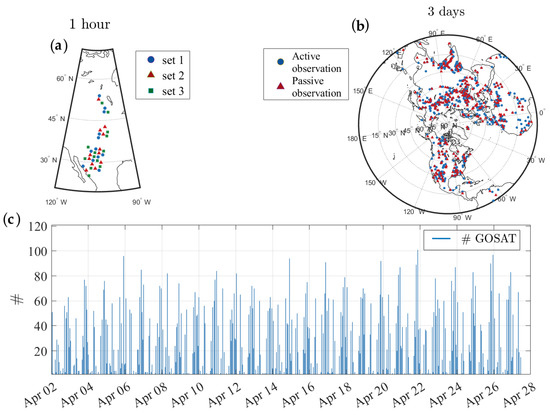
Figure 1.
Spatial and temporal distribution of GOSAT methane observations used in cross-validation. (a) 1-h GOSAT observations separated in three sets after thinning; (b) active observations (blue circles) versus passive observation (red triangles) over 3 days in the cross-validation framework to estimate the covariance parameters; (c) frequency of GOSAT observation per hour used in cross-validation.
Here we describe the experimental setup to estimate the covariance parameters. Three parameters, including , , and , are considered for the optimization problem using cross-validation cost-function (Equation (4)). We recall that observation, model, and initial error covariance are considered uniform and uncorrelated (see Section 4.4 of Part I [1] for details). The background error covariance adapts a homogeneous isotropic horizontal and vertical error correlation based on a second-order autoregressive (SOAR) correlation model (see Section 4.3 of Part I [1] for details). A series of hourly methane analyses are conducted for a period of two weeks (5 April to 18 April 2010), with 3 days spin-up of the assimilation system. This analysis is repeated to find the parameter optimum, altering from 200 km to 600 km with a step size of 50 km, from 0 to 13 vertical levels with increment, and from 0.1 to 1.2 with a 0.1 step size.
Simultaneous optimization of the three parameters as discretized above requires a total ensemble of assimilations of 1512, i.e., 9 × 14 × 12 = 1512, corresponding to the specified parameters, × × , in the optimization. Perhaps, other optimization techniques could resolve this problem more efficiently [41,42]. An iterative scheme is adapted instead, where and are estimated together while is considered separately. With the initial values of = 500 km, = , and = 1 taken as first guesses (Table 1, initial), the experiment is started for the estimation of while and are kept fixed. This essentially corresponds in searching for the that minimizes the cross-validation cost function (Equation (6)) while the innovation covariance consistency (Equation (1)) is respected. Note that the procedure is repeated for all three permutations of cross-validations subsets to ensure that all observations have been used for evaluation. The new estimate of is obtained by averaging for the three verifying subsets (Table 1, itr 0/step 1). The estimated ( = 0.45) is then used to estimate and together in the next step of zero iteration (Table 1, itr 0/step 2). The procedure is repeated for successive iterations until convergence. Nevertheless, it is established that a single iteration will be sufficient to reach convergence for a similar estimation method [30,31,43,44]. We also confirm this for our estimation problem as shown in the first iteration (itr 1) in Table 1 (itr 1/step 1 and itr 1/step 2). Thus, the number of computations declines to 2 × (9 × 14 + 12) = 276 for the same number of parameters and same step size of each parameter.

Table 1.
Comparison of the error variance parameters (, , and ) along with the cross-validation cost function generated with passive observations at different stages of iterative optimization, including the initial step, zero iteration (itr 0) and first iteration (itr 1). Each iteration contains two steps, one for optimizing (step 1) and another for optimizing and together.
Figure 2a and Figure 3 (red curve) illustrate the estimation of , , and , after the first iteration that corresponds to the minimum value with the specified optimization resolution in the cross-validation (i.e., passive observation) space. A cost function based on the active observations, , is constructed to compare with the cross-validation results. Figure 2b and Figure 3 (blue curve) represent the similar parameter estimation procedure described above, but over the active observations (i.e., training set). In Figure 3, the evaluation against active observations (blue curve) always shows smaller variances than the evaluation against passive observations (red curve). It implies that the use of active observations overestimates the performance (a well-known property of cross-validation optimization [31]) of the analysis. In addition, the use of passive observations in cross-validation results in the existence of a minimum variance cost-function, consistent with the finding of Ménard and Deshaies-Jacques (2018) [31].
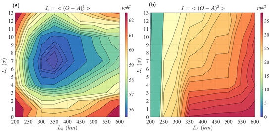
Figure 2.
Estimation of the horizontal length scale (, x-axis) and the vertical length scale (, y-axis) together through (a) a cross-validation cost function of passive observations and with (b) a cross-validation cost function of active observations .
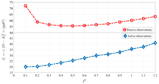
Figure 3.
Estimation of observation error variance parameter, , using a cross-validation cost function of passive observations (red curve) and using a cross-validation cost function of active observations (blue curve).
To verify that the cross-validation method using 10 km thinning of satellite observations yields the optimal parameter, we have conducted the same analysis as shown above, but this time against independent Total Carbon Column Observing Network (TCCON) observations. Note that TCCON is often considered as a reliable observation data set. However, their coverage is rather limited in space but continuous in time (seven sites only; see Section 5 for detail of TCCON observations). Figure 4 shows the comparison of analysis () using active GOSAT observations against TCCON (), which is an independent source of observation. The cross-validation cost function, , is drawn against the three parameters ( in the left, in the middle, and in the right panel of Figure 4). To save on the computation, we perform the estimation on each parameter individually. Figure 4 shows that the optimal parameter values obtained against TCCON are the same as those estimated through cross-validation (using GOSAT passive observations). Hence, despite the fact that cross-validation was developed for in situ observations, this result indicates that satellite observation thinning can indeed yield the optimal values. This example shows that the applicability of the cross-validation method [30,31] to the satellite observations is valid.
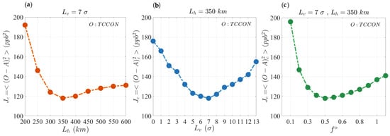
Figure 4.
Estimation of the (a) horizontal correlation length, , (b) vertical correlation length, , and (c) observation error covariance parameter, , using independent TCCON observations with the cross-validation cost function, .
4. Estimation of Model Error and Initial Error Variance Using Innovation Variance Consistency
By conducting the estimation presented in Section 3 on a different time window (e.g., a different two weeks period or a shorter/longer period), we found that the optimal estimation of the three parameters, , , and , is relatively insensitive to the time window of estimation. The model and initial error variances, on the other hand, (or their covariance parameter counterparts, and ) are excluded from our covariance parameter vector, , in the cross-validation optimization due to their time-varying influence (i.e., accumulating or decaying behaviour). In other words, having a different optimization time window results in a different set of optimized and . Thus, instead of including and in the time-insensitive parameter vector (), we tuned them separately using the variance matching diagnostic technique defined in Section 2 (Equation (1)). A description of the form of initial and model error covariance is presented in Section 4.4 of Part I [1].
First, we characterize a normalized variance matching diagnostic that offers a diagnostic independent of units and independent of the number of observations. The covariance matching diagnostic, reformulated as the total variance matching, can be written as
The normalized variance matching diagnostic is then obtained by dividing the right-hand side of Equation (9) with the number of observations, , and representing the variance at a specific observation location or the mean of all observations. Thus, we have
Writing the diagnostic in this fashion removes the dependency of the diagnostic to the absolute statistics, so that it retains a similar form to other diagnostics such as χ2 [45]. Therefore, a proper model error in our estimation system is obtained when it satisfies the near-zero normalized variance matching with continuous stability over time. Figure 5 illustrates the influence of the model error on this diagnostic. A small (Figure 5a) leads to an increasing pattern () over time, whereas a large (Figure 5c) results in a decrease (); both of them tend to disagree with the innovation variance consistency over time. A proper value of = 0.018 (Figure 5b) can be found with trial and error that fulfills the innovation variance consistency. Note that the initial error variance parameter is kept constant = 0.45 for all cases, while it is shown for its best estimate (see Figure 6).
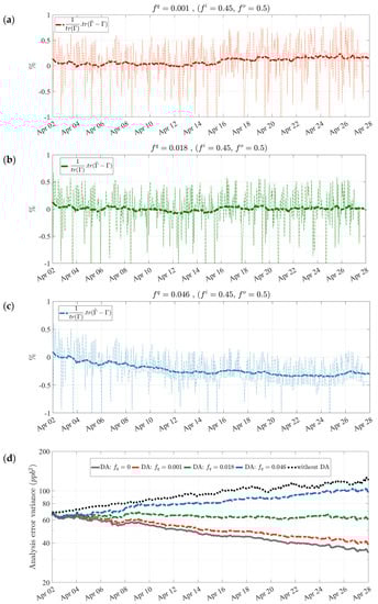
Figure 5.
Normalized innovation variance consistency diagnostic for a (a) low ( = 0.001), (b) proper ( = 0.018), and (c) high ( = 0.046) model error parameter value. (d) Indicates the effect of model error on analysis error variance over time.
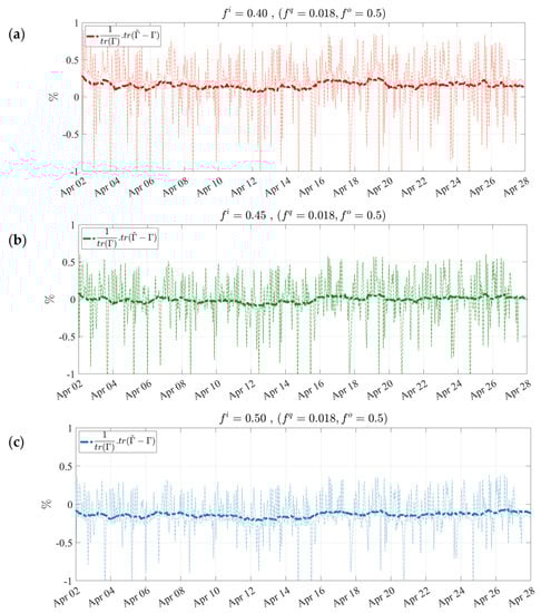
Figure 6.
Normalized innovation variance consistency diagnostic for a (a) low ( = 0.40), (b) proper ( = 0.45), and (c) high ( = 0.50) initial error parameter value.
Furthermore, we verify the influence of the model error on the analysis error variance in Figure 5d. Both cases of “without DA” and perfect model or ( = 0) produce too small or too large analysis error variance as time proceeds, causing degraded assimilation results with overestimation or underestimation implications. Therefore, the presence of a certain amount of model error is crucial. As found in the diagnostic above, we infer that the proposed model error parameter ( = 0.018) also maintains a stable analysis error variance over time.
We repeat the same diagnostic experiment to obtain an appropriate . We note that different values of are considered initially for this test, and the best value, = 0.018, which maintains a stable diagnostic, is shown in Figure 6. Figure 6 suggests that = 0.45 meets the condition of innovation variance consistency, although it may not reach the final error variance within two weeks to show asymptotic stability of the Kalman filter estimation (see Jazwinski (1970) [46], Theorem 7.4). We infer that the thinned GOSAT data used in this study may produce an analysis that induces a lack of observability (e.g., see Jazwinski (1970) [46], Section 7.5 for the definition of observability). Nonetheless, we have all the parameters that lead to an optimal analysis and to innovation variance consistency. Those estimated parameters are close to the true error variance parameters.
5. Evaluation against Independent Observations
The optimal analysis can be obtained as a result of successful assimilation. This relies not only on the assimilation processes but specifically on the proper characterization of the input error parameters. The observation error covariance (), the model error covariance (), and in some cases, the initial error covariance (), besides the error correlation length scales, are among those determined in the PvKF assimilation. Hence, the optimality of the analysis depends on how precisely the Kalman filter error covariances (, ) reflect the true estimation of error covariance parameters. We recall the definition and the formulation of the input error covariances in Part I, Section 4.4 [1].
The assimilation results shown in Section 5 and Section 6 are produced with thinned GOSAT data that pass all quality control flags (e.g., retrieval flag, outliers), maintaining about 35–50% of all GOSAT retrievals for assimilation. Accordingly, the desired assimilation involves globally optimized (or quasi-optimal) error parameters, including , , , and . After finding these optimized error parameters, as discussed in Section 3 and Section 4, independent measurements from multiple sources are used to evaluate the assimilation performance. Figure 7 demonstrates the location/pathways of all surface/aircraft available measurements collected for the duration of our assimilation results in April 2010. Below, we provide a brief description alongside the preparation of these independent observations.
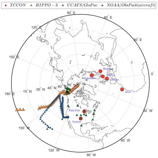
Figure 7.
Methane measurement data used for the evaluation of the assimilation system in April 2010: TCCON stations (red circles) at seven sites; HIPPO-3 aircraft measurement pathways (orange triangles) on 10, 13 and 15 April 2010; UCATS/GloPac aircraft measurement pathways (blue triangles) on 7 and 13 April 2010; and NOAA/Obspack aircraft measurements (green triangles).
TCCON is a ground-based FTS network that provides a time series of CH4 column-averaged abundance worldwide. TCCON data has been used to compare with model simulations and satellite data primarily for validation purposes [15,47,48,49,50,51,52]. We used the GGG2014 version of TCCON XCH4 data from seven sites (red circles in Figure 7), including Park falls [53], Orleans [54], Lamont [55], Bremen [56], Sodankyla [57], Izana [58], and Bialystok [59], available at https://tccondata.org/2014 (accessed on 14 November 2021). TCCON is calibrated using aircraft profiles to maintain better than 0.5% accuracy of XCH4 retrievals [60]. Prior to the comparison with the model or analysis, we convolve CMAQ with TCCON average kernels and the corresponding a priori profiles, for which the procedure is described in Wunch et al. (2010) [61] or through the website https://tccon-wiki.caltech.edu/Main/AuxilaryData (accessed on 14 November 2021). Similar to the aircraft measurements described later in this section, TCCON retrievals are assumed to provide an independent evaluation for our assimilation results. This is due to the fact that TCCON is neither used in generating the model input nor in calibrating the GOSAT data with CMAQ. We recall that GOSAT data are bias-corrected against only surface measurements of GLOBALVIEWplus CH4 ObsPack v3.0 as described in Sections 4.1 and 4.2 of Part I [1]. Therefore, any influence of TCCON calibration on GOSAT data prior to this study will be entirely alleviated. Note that we employed the same latitudinal correction on TCCON as we used for GOSAT to ensure a consistent comparison with independent observations.
HIAPER Pole-to-Pole Observations (HIPPO-3) are among the five HIPPO aircraft missions that provide methane concentration measurements [62] from surface to 14 km across the Pacific Ocean between 20 March and 20 April 2010. The measurement is conducted every second using a quantum cascade laser spectrometer (QCLS) with an accuracy of 1 ppb. Methane measurements, meteorology and flight tracking data are accessible at: https://www.eol.ucar.edu/field_projects/hippo (accessed on 14 November 2021). For the North Hemisphere, the measurement data are available on 10, 13 and 15 April 2010, as shown by orange triangles in Figure 7. To compare with HIPPO-3, we interpolate the model concentration at the specific location, height, and time of the measurement. The significantly shorter time scale of the measurements (i.e., 1 s) compared to the model simulation time step (i.e., 1 h) allows a larger variation, resulting in a degraded comparison with the model or analysis at the observation space. Therefore, with the aim of meaningful comparison, we exclude those HIPPO-3 data that depart by more than three standard deviations from the average measurement over one minute or 60 consecutive measurements. This results in removing 58% of the total HIPPO-3 data as the outliers for this comparison.
Global Hawk Pacific (GloPac) is an aircraft mission operated by NASA in April 2010 primarily designed to validate monitoring satellite missions and to measure trace gases in the upper troposphere and lower stratosphere. UAS Chromatograph for Atmospheric Trace Species (UCATS) was integrated into GloPac to measure methane alongside N2O, SF6 and several other trace gases. It offers an overall precision of 0.5% for methane [63]. All the data are available at https://espoarchive.nasa.gov/archive/browse/glopac (accessed on 14 November 2021), where the methane measurements were recorded on 7 and 13 April 2010 with a time resolution of 140 s and are shown in Figure 7 by blue triangles. Note that we use methane measurements without filtering, and the model and analysis are computed at every measurement.
GLOBALVIEWplus ObsPack v3.0 data product [64] published via NOAA Global Monitoring Laboratory provides high accuracy measurements of methane concentration from a variety of sampling platforms, including surface, tower, aircraft, and shipboard measurements. Since the surface flask and tower data are used in the calibration of GOSAT (see Sections 4.1 and 4.2 of Part I [1]), we only use ObsPack aircraft data to ensure an unbiased comparison with the analysis. Accordingly, only daily above 800 m from the dataset of ObsPack available at (https://gml.noaa.gov/ccgg/obspack/ (accessed on 14 November 2021)) is used to represent the aircraft measurements, which are collected from multiple aircraft campaigns [64]. These measurements are demonstrated by green triangles in Figure 7.
Before evaluating the performance of the optimal analysis against independent observations, we highlight the differences between an optimal and nonoptimal analysis. Accordingly, under similar conditions (e.g., model configuration, inputs), the optimal analysis is compared against another analysis produced with an arbitrary, yet commonly used, nonoptimal set of parameters. The globally optimized parameters in April 2010, as described in Section 3 and Section 4, consist of = 0.5, = 0.45, = 0.018, = 350 km, = , whereas the arbitrary parameters include = 1.2, = 0.45, = 0, = 600 km, = , for the nonoptimal case. Figure 8 demonstrates the comparison of model forecast without data assimilation (blue circles), analysis with optimal parameters (red circles), and analysis with nonoptimal parameters (green circles) against independent TCCON observations. The results indicate that both and the regression slope are the smallest for the nonoptimal analysis while the mean bias is the largest. It suggests that the nonoptimal analysis generated with a set of arbitrary, but typically used, parameters could result in an agreement even worse than the model against independent measurements. This behaviour was also found for the analysis of PM2.5 with surface observations [30]. On the contrary, the optimal covariance parameters produce an analysis that maintains a significantly higher consistency with TCCON observations than the model without assimilation. Similar results are obtained with other types of independent observations and a different set of arbitrary (nonoptimal) parameters (see Figures S1–S6 in the Supplementary Materials). Thus, it could be inferred that proper estimation of error covariance parameters is essential for PvKF assimilation and most data assimilation schemes that also depend on those input error covariance parameters (e.g., 4D-Var, EnKF).
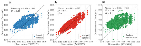
Figure 8.
(a) Comparison of model forecast (blue circles), (b) analysis with optimal parameters (red circles), and (c) analysis with nonoptimal parameters (green circles) against independent TCCON observations. Optimal parameters of the analysis include = 0.5, = 0.45, = 0.018, = 350 km, = and the nonoptimal parameters are assumed to be = 1.2, = 0.45, = 0, = 600 km, = .
The GOSAT methane assimilation with optimized parameters is further examined by comparing it with the model forecast against all four types of independent measurements, including TCCON (Figure 9a), HIPPO-3 (Figure 9b), NOAA/ObsPack aircraft (Figure 9c), and UCATS/GloPac (Figure 9d) as shown in Figure 6. In Figure 9, the blue circles (model) represent a pure forecast simulation of H-CMAQ between 2 to 28 April 2010, whereas the red circles (analysis) denote GOSAT assimilation with optimized parameters, both of which are sampled at the same measurement location and time and using the same model inputs and configuration. The analysis shows an overall and consistent improvement in agreement with all four types of independent measurements, even though the level of improvement is not the same for all of them. Furthermore, among those four observations, analysis at TCCON and NOAA/ObsPack aircraft, which are located over land, shows a relatively better agreement due to higher correlation and a narrower spread of data points. This implies that constructing the analysis using land-only GOSAT data with high retrieval quality reflects a better consistency with independent land measurements. Nevertheless, the analysis maintains a better agreement than the model with HIPPO-3 and UCATS/GloPac, located mainly over the ocean where no GOSAT observations were used. It can be inferred that the evolution of error variance using an advection scheme enhances the assimilation capabilities to maintain a relatively higher consistency with independent observations within a short period of time, even far from the observations used to generate the analysis.
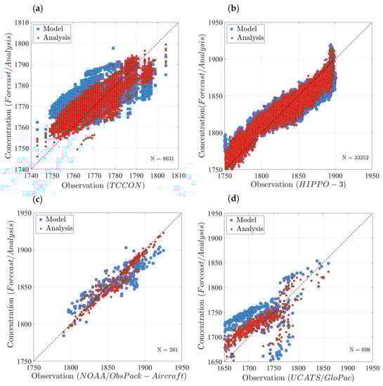
Figure 9.
Comparison between the model forecast (blue circles) and analysis with GOSAT assimilation (red circles) sampled at four types of independent measurements, including (a) TCCON, (b) HIPPO-3, (c) NOAA/ObsPack aircraft, and (d) UCATS/GloPac. N denotes the number of observations of each type.
Comparison of the model () and analysis () statistics for each type of measurement are listed in Table 2 and emphasize the benefit of using the assimilation with optimal parameters. The largest improvement of the correlation () along with a reduction of mean bias () and standard deviation () is observed at TCCON locations ( = +39.9% or = 2.1), followed by NOAA/ObsPack aircraft measurements ( = +13.9% or = 1.18). These two observations both occur over land and differ in their vertical sampling, where TCCON measures the total column, and NOAA/ObsPack provides point measurements from the mid-troposphere up to the lower stratosphere [64]. Using TCCON, the analysis is capable of detecting the total methane bias, whether due to incorrect surface emissions or modelling errors of unknown origin. In contrast, the bias of the analysis relative to NOAA/ObsPack aircraft can isolate the impact of modelling errors on the analysis since little of the emissions signal reaches aircraft measuring altitude (i.e., several thousand kilometers) within a short period of time (i.e., several weeks). The positive bias of the forecast model with respect to TCCON contrasted with its negative bias relative to NOAA/ObsPack suggests that an excessive amount of surface emissions or high tropospheric methane background is incipient in H-CMAQ, while methane abundance is underestimated in the upper troposphere and lower stratosphere.
Table 2.
Evaluation of model forecast (M) and analysis (A) of GOSAT assimilation against TCCON, HIPPO-3, UCATS/GloPac, and NOAA/ObsPack measurements. Comparison between mean bias (MB), standard deviation σ, coefficient of determination R2, and the linear regression line, using all measurements of each type of observation in April 2010.
Knowing that the analysis increments are driven by emissions at or near the surface or from modelling errors, we can attempt to qualitatively identify the significance of this influence from each one of these sources. We recall that evaluation with TCCON could show a combined emissions and modelling error effect, while NOAA/ObsPack only corresponds more closely to the bias originating from modelling error. The analysis increments statistics at TCCON and NOAA/ObsPack show a 39.9% and 13.9% increase of , respectively. The mean bias also denotes an improvement of 3.51 ppb with TCCON, and 1.32 ppb with NOAA/ObsPack. It could be inferred that the global influence of the surface emissions is more significant than the modelling error due to a significant improvement of both and against TCCON rather than NOAA/ObsPack. It is worth mentioning that the model is also less capable of predicting methane concentration over land than over the ocean, mainly due to incorrect model emissions generated from the land surface. This explains the lowest model correlation against TCCON with total column measurements (Table 2) compared to the other 3 observations at higher altitudes and mainly over the ocean. Accordingly, the analysis correlation against TCCON has remained lower than the other 3 observations; however, we remark the largest correlation improvement in the analysis against TCCON. We discuss later in Section 6 the spatial distribution of the analysis increment and error variance reduction. Note that our analysis evaluation with TCCON stations shows a comparable result to the weak-constraint 4D-Var in the global GEOS-Chem data assimilation employed by Stanevich et al. (2021)—Table 1 [15].
Comparing the model and analysis at HIPPO-3 and UCATS/GloPac, both taken over the Pacific Ocean, shows a reduction of 66% and 41% in MB alongside a 3.7% and 6.8% increase of R2, respectively (Table 2). The forecast model sampled at HIPPO-3 locations exhibits a negative bias relative to the observations, representing a combined tropospheric and lower stratospheric bias between 0.9 km and 13 km altitude. Addressing the origin of this bias is not a trivial task; however, our analysis successfully removed a significant portion of that. Given an unbiased initial condition and the small impact of emissions over the HIPPO-3 domain, we relate this bias to modelling error originating primarily from the oxidation of methane with OH in the troposphere [6,65], methane stratospheric transport [52], and methane oxidation with chlorine radical over the Oceans [66]. The model and analysis evaluation at UCATS/GloPac aircraft measurement locations reveals a large positive bias that contradicts the earlier comparison results with HIPPO-3 and NOAA/ObsPack aircraft measurements. This disagreement likely arises from the limited vertical structure of H-CMAQ extended up to 50 hPa (~20 km), which cannot entirely and adequately cover all the measurements. In fact, GloPac aircraft is mainly flying over the lower stratosphere [63,67], for which quite a few measurements are recorded beyond or at the few top layers of H-CMAQ. Therefore, in addition to the sources of modelling error mentioned earlier, inter/extrapolation of model concentration at these measurements’ height adds up to the positive bias, which is unrealistic. Nonetheless, our analysis could remove a noticeable part of this bias, whether from a physical model bias (e.g., part of the stratospheric bias) or an artificial bias (e.g., numerical inter/extrapolation).
Several studies provide in-depth investigations of the possible causes of methane model bias in a global atmospheric model (e.g., GEOS-Chem), such as stratospheric bias [10,15,37,52,68], weakening of vertical transport due to a coarse model resolution [14], OH burden in the chemistry model [6,9,65,69]. Besides those, H-CMAQ could suffer from bias due to inaccurate initial conditions, insufficient lower top of the model boundary conditions, and interhemispheric exchange of methane. Uncovering the origins of the model bias and distinguishing it from surface emissions bias requires an exhaustive forward and/or adjoint sensitivity analysis besides identifying all the possible sources of uncertainty, which is out of the scope of this study. Still, the discrepancy between the optimal analysis and the model (i.e., analysis increment) together with the uncertainty reduction can reveal useful information to address the key sources of bias and uncertainty associated with methane simulation. We illustrate these in Section 6, both in the H-CMAQ and GOSAT observation space.
6. Characteristics of Analysis and Error Variances
This section examines the performance of our analysis with optimal parameters in capturing the spatial structure of bias and uncertainty reduction across the domain. First, we compare one month of analysis against the model forecast in the observation space, where model and analysis are sampled at GOSAT times and locations with an identical observation operator. A difference between model/analysis and GOSAT is shown in Figure 10. Comparing Figure 10a,b indicates that a significant portion of biases in the model from different parts of the world, including a positive bias at eastern China, India, eastern parts of Russia, South Asia, tropical and eastern Africa, northern Europe, eastern Canada, and the western U.S. are substantially removed by the analysis. At the same time, the analysis also resolves the negative bias in areas such as northern Africa, eastern Europe, and the southeastern U.S. Accordingly, the analysis demonstrates an 80% and 65% adjustment over the areas with the largest positive and negative model bias, respectively. A direct comparison between the analysis and the model is also shown in Figure 10c, indicating the consistency of the analysis with GOSAT retrievals to correct the spatial variation of the biases.
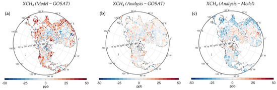
Figure 10.
Differences between (a) model and GOSAT, (b) analysis and GOSAT, and (c) analysis and model in the observation space in April 2010.
The methane spatial bias in many studies is primarily attributed to its prior emissions allocation and is resolved using inverse modelling analysis [10,37,38,52,70]. The bias can also arise from the limitation of the chemical transport model to realistically simulate atmospheric methane, also known as the bias due to model error [14,15,68,71]. The optimal analysis described in this study corrects for these biases and assists in identifying the origins of these biases. Continuous real-time estimation of assimilated methane concentration alongside its error variance reduction enables a direct and reliable comparison with the model forecast, which reveals valuable information. It is common to consider over a short period of time (e.g., one month) that the analysis increment at the surface reflects the correction needed for improving the prior surface emissions while the increments at the higher elevations (e.g., <500 hPa) is due to the combined effect originated from model error and inaccurate emissions. Furthermore, the analysis error variance reduction computed here by PvKF represents the analysis uncertainty, thus is an indicator of assimilation accuracy with respect to the true state.
The monthly average of the analysis, analysis increments (i.e., Analysis − Model), and the analysis error variance reduction at the surface and 550 hPa are shown in Figure 11. We found that the largest downward correction occurs over Russia, while the largest upward correction is over tropical Africa (Figure 11b). These results are consistent overall with recent methane inverse studies; for example, Wang et al. (2019) [8] considered a 200% downwards adjustment to the prior emissions over Russia from EDGAR. Zhang et al. (2021) [52] estimated Russia’s anthropogenic emissions to be about 59% of its prior value, mainly attributed to the oil-and-gas sector. In the same study, a large upward correction in the prior inventory is also reported over East and tropical Africa, mainly due to the growth of livestock and wetland emissions. Our analysis at the surface also suggests a positive bias over India, Japan, eastern China, Europe, high latitudes, western U.S. and all over Canada, whereas a comparatively negative bias over the South and Southeastern U.S., northern regions of South America, and Central Asia. Note that several factors such as the discrepancy between emission inventories, the atmospheric model, and the temporal variations can explain slight differences between studies. In addition, the correction near the Equator in our hemispheric assimilation could be too diffusive to constrain the spatial pattern of the bias on regions next to the Equator; hence, all plots in Figure 10 and Figure 11 are shown above 5°N.
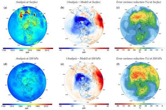
Figure 11.
(a) Monthly analysis at the surface and (d) at 550 hPa; (b) analysis increment at the surface and (e) at 550 hPa; (c) error variance reduction at the surface and (f) at 550 hPa.
Above those regions with maximum and minimum values of the analysis increment at the surface, the analysis increment at 550 hPa (Figure 11e) suggests a similar scale and pattern of correction in most regions over North America and Africa. However, there is a noticeable discrepancy over the lower and mid-latitude Pacific Ocean, East Asia, India, and the Middle East, where the analysis suggests a positive correction in the mid-troposphere rather than the negative correction captured at the surface. As suggested by Stanevich et al. (2021) [15], we consider the vertical dipole structures in our analysis increment as the cause of modelling error in the bias, whereas a monotonic correction represents the impact of the inaccurate emissions on the bias. Another region of interest is the eastern part of the Atlantic Ocean, where the analysis increment is significantly larger at 550 hp than the surface, yet with the same correction sign (Figure 11e). That possibly indicates the presence of model error over those regions, where convection does not lift up enough methane to the mid and upper troposphere in H-CMAQ, partly due to a persistent high-pressure and low-pressure system in the African continent. Such a pattern is also observed in previous global studies with different chemistry transport models [15,72,73].
As a distinctive feature, the analysis error variance is explicitly computed by the PvKF assimilation. It represents the estimation uncertainty with respect to the true state, thus inferring how reliable the assimilation results (i.e., 3D optimal analysis) are. The spatial distribution of the analysis increment is mainly influenced by the innovation (Observation—Model), whereas the distribution of the analysis error variance depends largely on the observation density and its error. This discrepancy arises from the fact that the analysis of the second moments (i.e., error covariances) is decoupled from the first moment (i.e., mean state) in linear Kalman filtering estimation theory [74]. In the upper troposphere (i.e., 550 hPa), the spatial pattern of error variance reduction (Figure 11f) is more consistent with the analysis increment (Figure 11e), such that a larger reduction of error variances occurs over the same regions with larger analysis increment, suggesting that those corrections are fairly reliable. In contrast, the spatial distribution of the error variance reduction at the surface (Figure 11c) is not always following the analysis increment spatial pattern (Figure 11b). For instance, the analysis over North/East Africa shows the largest increase while the error variance reduction is relatively small, indicating that the analysis correction over those regions is less reliable. It could be implicitly inferred that conducting emissions inversion over these areas would entail higher uncertainty in corrected emissions.
Since the analysis provides us with an hourly real-time assimilated methane with GOSAT, it is interesting to examine its time series and compare it with equivalent model values. Figure 12 shows the analysis and the model values projected to the six TCCON observations sites (red circles in Figure 7), using the TCCON averaging kernels and a priori. In the time series plots, the green dots denote the TCCON observations, while the red and blue dots represent the analysis and model values, respectively. Note that TCCON averaging kernels are fairly smooth and vary only slightly with solar zenith angles and pressure [61], so that we averaged those values of two consecutive measurements in order to provide a continuous model and analysis over time.
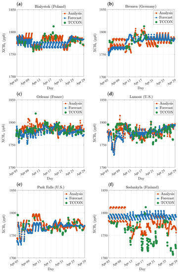
Figure 12.
Comparison of the time series of the analysis (red dots) and the model (blue dots) against TCCON observations (green dots). Six TCCON observation sites (Figure 7—red circles) include (a) Bialystok (53.23°N, 23.03°E), (b) Bremen (53.10°N, 8.85°E), (c) Orleans (47.97°N, 2.11°E), (d) Lamont (36.60°N, 97.48°W), (e) Park Falls (45.95°N, 90.27°W), (f) Sodankylä (67.37°N, 26.63°E).
We showed earlier (Figure 9) that the analysis with optimal parameters maintains a significantly better agreement with TCCON. The spatial distribution of the optimal analysis is also consistent with GOSAT retrievals (Figure 10) and agrees with the recent findings of methane inversion studies. The times series plots (Figure 12) indicate that the analysis also follows the temporal variation of independent measurements, whereas the model forecast is almost insensitive to these variations. For example, at the Sodankylä observation site (Figure 12f), TCCON shows a consistent temporal pattern measuring between 1710 to 1770 ppb from 13 to 29 April 2010. The model shows no sign of agreement with TCCON over the same period; however, the analysis attempts to correct the model toward these independent measurements depending on the feedback provided by GOSAT observation for methane assimilation.
We should note that the analyses in Figure 12 are optimized with the error parameters obtained in Section 3 and Section 4. Similar to the evaluation of optimal and nonoptimal analysis with TCCON (Figure 8), we compare the time series of those two cases (using the same set of optimal and nonoptimal error covariance parameters) at Sodankylä. As shown in Figure 13, an analysis obtained with a set of nonoptimal, yet commonly used, error covariance parameters (black dots) can result in an even worse temporal agreement with TCCON (See Figures S7 and S8 in the Supplementary Materials for more examples). Therefore, we conclude once more that obtaining the optimal error covariance parameters is essential to have a reliable analysis that improves the methane representation both spatially and temporally.
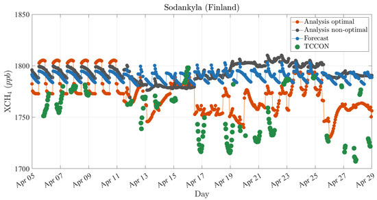
Figure 13.
Comparison of model forecast (blue dots), analysis with optimal parameters (red dots), analysis with nonoptimal parameters (black dots) against Sodankylä (67.37°N, 26.63°E) TCCON observations (green dots). Optimal parameters of the analysis include = 0.5, = 0.45, = 0.018, = 350 km, = and the nonoptimal parameters are assumed to be = 1.2, = 0.45, = 0, = 600 km, = .
7. Conclusions and Summary
We employed the PvKF data assimilation scheme developed in Part I to the GOSAT observations in the hemispheric CMAQ domain to produce a high-quality (i.e., near-optimal) analysis of atmospheric methane concentration. Although most assimilation schemes such as PvKF are derived from minimum variance estimation theory, it does not mean that the analysis produced using real observations will be the best one. The input error covariances (e.g., observation error covariance, model error variance and correlation lengths) also need to be realistic. In this paper, we used several techniques to obtain accurate error covariances and show, using independent observations and cross-validation, that these realistic error covariances indeed achieve better analyses. For example, of independent TCCON observations with analysis is 0.29 when using inaccurate error covariances and increases to 0.75 with optimal error covariances.
In this work, the cross-validation methodology developed originally for in situ observations [31] has been extended for satellite observations using observation thinning. In fact, we have verified that thinned satellite observations (10 km apart) give the same optimal parameter values as those obtained with independent TCCON observations. Our procedure is not to estimate all elements of covariance matrices (since it requires an extremely large number of data or realizations), but rather a few key global parameters of these covariances. We have estimated the horizontal and vertical correlation lengths of the background error covariance and the observation error variance. It is important to note that the cross-validation estimation technique is the desired approach since it does not assume that the analysis is (already) optimal. Thus, the covariance parameter optimization results in realistic error covariances and near-optimal analyses. We recall that optimal analyses and innovation covariance consistency are the necessary and sufficient conditions to estimate true observation and background error covariances [28]. We also found that these error parameters are nearly insensitive to the optimization time window, so that they are valid for the entire month of assimilation of this study. On the contrary, the cross-validation is not properly applicable to estimate the model and initial error variances due to a noticeable time-varying influence on the optimization window. We demonstrate a normalized variance matching diagnostic approach to tune these parameters while maintaining a stable analysis error variance. Finally, we note that the optimization approach of this study is applicable to any other assimilation experiment but may result in different correlation length scales with different observation densities.
Once the optimal analysis using GOSAT is obtained, we evaluate the analyses against different types of independent observations (TCCON, NOAA/ObsPack, UCATS/GloPac, HIPPO-3). We show its superiority against analysis produced using reasonable but arbitrary values of covariance parameters. Furthermore, the comparison between model (with no assimilation) and optimal analysis against TCCON and NOAA/ObsPack suggest an overestimation of surface methane (most likely due to emissions) and an underestimation of the upper-tropospheric model methane. Remarkably, our PvKF assimilation is capable of correcting both of these biases regardless of their origin. The correction’s statistics due to assimilation are more significant with respect to TCCON, which is a total column measurement, than with respect to NOAA/ObsPack, which only samples the upper troposphere. This suggests that the assimilation of GOSAT makes the larger correction near the surface, where presumably there are larger errors than the upper troposphere. The assimilation of GOSAT also seems capable of addressing the known model problem in the horizontal direction. For instance, our analysis increment suggests the largest negative correction over Russia, whereas the largest positive correction over tropical Africa. This is coherent with the recent methane inverse studies [15,52]. Furthermore, we have a large reduction of error variance over those regions, suggesting that those corrections are reliable. In addition, the PvKF assimilation that offers a time-continuous series of analyses enables us to investigate the temporal behaviour of the model biases. Our results show a better temporal agreement between analysis and TCCON than between model (no assimilation) and TCCON. In summary, it appears that the optimal assimilation of GOSAT is able to correct for the vertical, horizontal, and temporal model errors as revealed by comparison with independent observations.
Because this assimilation system provides the state estimate and its error, it is suitable to couple it with another estimation problem such as a limited domain data assimilation, source inversion, etc. In theory, the PvKF formalism also seems to be applicable to the joint assimilation-inversion (state-source estimation) problem, but we need to demonstrate that in a realistic context, which will be considered in a future manuscript. This method could also be applied to chemical species with a shorter lifetime, knowing that a smaller fraction of the total forecast error variance is explained by the advection of error variance. In this case, more (unexpected) error variance is carried out with a stationary model error, which emphasizes a more sophisticated design of the model error covariance. Therefore, a shorter lifetime of a chemical species may induce a weaker performance of the PvKF assimilation and make it behave closer to an Optimal Interpolation (OI). Another application of the PvKF assimilation that could be investigated in future studies is to use the analysis over the oceans to develop the bias correction of GOSAT over ocean observations.
Supplementary Materials
The following supporting information can be downloaded at: https://www.mdpi.com/article/10.3390/rs14020375/s1, Figure S1: (a) Comparison of (a) model forecast (blue circles), (b) analysis with optimal parameters (red circles), and (c) analysis with nonoptimal parameters (green circles) against independent NOAA/ObsPack aircraft observations. Figure S2: Comparison of (a) model forecast (blue circles), (b) analysis with optimal parameters (red circles), and (c) analysis with nonoptimal parameters (green circles) against independent UCATS/GloPac observations. Figure S3: Comparison of (a) model forecast (blue circles), (b) analysis with optimal parameters (red circles), and (c) analysis with nonoptimal parameters (green circles) against independent HIPPO-3 observations. Figure S4: Comparison of (a) nonoptimal analysis due to only correlation lengths larger than the optimal value (e.g., ), (b) optimal analysis with optimal correlation lengths (i.e., ), and (c) nonoptimal analysis due to only correlation lengths smaller than the optimal value (e.g., ). Figure S5: Comparison of (a) nonoptimal analysis due to only observation error smaller than the optimal value (e.g., ), (b) optimal analysis with optimal observation error (i.e., ), and (c) nonoptimal analysis due to only observation error larger than the optimal value (e.g., ). Figure S6: Comparison of (a) nonoptimal analysis due to only model error smaller than the optimal value (e.g., ), (b) optimal analysis with optimal model error (i.e., ), and (c) nonoptimal analysis due to only model error larger than the optimal value (e.g., ). Figure S7: Comparison of model forecast (blue dots), analysis with optimal parameters (red dots), and analysis with nonoptimal parameters (black dots) against TCCON observations (green dots) at Lamont (36.60°N, 97.48°W). Optimal parameters of the analysis include and the nonoptimal parameters are assumed to be . Figure S8: Comparison of model forecast (blue dots), analysis with optimal parameters (red dots), and analysis with nonoptimal parameters (black dots) against TCCON observations (green dots) at Bremen (53.10°N, 8.85°E). Optimal parameters of the analysis include and the nonoptimal parameters are assumed to be .
Author Contributions
Conceptualization, S.V. and R.M.; methodology, S.V. and R.M.; software, S.V.; formal analysis, S.V.; investigation, S.V.; writing—original draft preparation, S.V. and R.M.; writing—review and editing, R.M., T.W.W. and A.H.; visualization, S.V.; supervision, R.M., T.W.W. and A.H. All authors have read and agreed to the published version of the manuscript.
Funding
This research received no external funding.
Institutional Review Board Statement
Not applicable.
Informed Consent Statement
Not applicable.
Data Availability Statement
The GOSAT satellite data are available from the European Space Agency Greenhouse Gases Climate Change Initiative at http://cci.esa.int/ghg (accessed on 5 November 2021). The GLOBALVIEWplus CH4 ObsPack v3.0 data product is available at www.esrl.noaa.gov/gmd/ccgg/obspack/data.php?id=obspack_ch4_1_GLOBALVIEWplus_v3.0_2021-05-07 (accessed on 5 November 2021) (Cooperative Global Atmospheric Data Integration Project, 2019). The TCCON data are available at https://tccondata.org/2014 (accessed on 14 November 2021) (TCCON, 2014). Each TCCON data set used in this study is individually cited and provided in the reference list. The HIPPO-3 aircraft data are available at https://www.eol.ucar.edu/field_projects/hippo/ (accessed on 14 November 2021). GloPac aircraft data are available at https://espoarchive.nasa.gov/archive/browse/glopac/ (accessed on 14 November 2021). EDGAR v6 anthropogenic emission inventories are available at https://edgar.jrc.ec.europa.eu/dataset_ghg60 (accessed on 5 November 2021) (European Commission, 2021). Modelling data and the source code for PvKF assimilation have been deposited in GitHub, https://github.com/Sinavo/PvKF_crv_methane.git (accessed on 5 November 2021). Additional information related to this paper may be requested from the corresponding author: Sina Voshtani (Seyyedsina.Voshtani@ec.gc.ca).
Acknowledgments
The authors of this paper acknowledge all of the data providers and laboratories (https://search.datacite.org/works/10.25925/20210401, accessed on 4 November 2021) that contributed to the GLOBALVIEWplus CH4 ObsPack v3.0 data product compiled by NOAA Global Monitoring Laboratory. We also greatly appreciate the free use of methane emissions data from the Emissions Database for Global Atmospheric Research (EDGAR) (https://edgar.jrc.ec.europa.eu/index.php/dataset_ghg60, accessed on 4 November 2021). Simulations for this study were performed on computational resources of Compute Canada (http://www.computecanada.ca, accessed on 4 November 2021).
Conflicts of Interest
The authors declare no conflict of interest.
References
- Voshtani, S.; Ménard, R.; Walker, T.W.; Hakami, A. Assimilation of GOSAT methane in the hemispheric CMAQ. Part I: Design of the assimilation system. Remote Sens. 2022; accepted. [Google Scholar]
- Ganesan, A.L.; Schwietzke, S.; Poulter, B.; Arnold, T.; Lan, X.; Rigby, M.; Vogel, F.R.; van der Werf, G.R.; Janssens-Maenhout, G.; Boesch, H.; et al. Advancing Scientific Understanding of the Global Methane Budget in Support of the Paris Agreement. Glob. Biogeochem. Cycles 2019, 33, 1475–1512. [Google Scholar] [CrossRef]
- Miller, S.M.; Michalak, A.M.; Detmers, R.G.; Hasekamp, O.P.; Bruhwiler, L.M.P.; Schwietzke, S. China’s coal mine methane regulations have not curbed growing emissions. Nat. Commun. 2019, 10, 303. [Google Scholar] [CrossRef] [PubMed]
- Turner, A.J.; Frankenbergb, C.; Wennberg, P.O.; Jacob, D.J. Ambiguity in the causes for decadal trends in atmospheric methane and hydroxyl. Proc. Natl. Acad. Sci. USA 2017, 114, 5367–5372. [Google Scholar] [CrossRef] [PubMed]
- Turner, A.J.; Jacob, D.J.; Benmergui, J.; Brandman, J.; White, L.; Randles, C.A. Assessing the capability of different satellite observing configurations to resolve the distribution of methane emissions at kilometer scales. Atmos. Chem. Phys. 2018, 18, 8265–8278. [Google Scholar] [CrossRef]
- Turner, A.J.; Frankenberg, C.; Kort, E.A. Interpreting contemporary trends in atmospheric methane. Proc. Natl. Acad. Sci. USA 2019, 116, 2805–2813. [Google Scholar] [CrossRef]
- Saunois, M.; Stavert, A.R.; Poulter, B.; Bousquet, P.; Canadell, J.G.; Jackson, R.B.; Raymond, P.A.; Dlugokencky, E.J.; Houweling, S.; Patra, P.K.; et al. The Global Methane Budget 2000–2017. Earth Syst. Sci. Data 2020, 12, 1561–1623. [Google Scholar] [CrossRef]
- Wang, F.J.; Maksyutov, S.; Tsuruta, A.; Janardanan, R.; Ito, A.; Sasakawa, M.; Machida, T.; Morino, I.; Yoshida, Y.; Kaiser, J.W.; et al. Methane Emission Estimates by the Global High-Resolution Inverse Model Using National Inventories. Remote Sens. 2019, 11, 2489. [Google Scholar] [CrossRef]
- Zhao, Y.H.; Saunois, M.; Bousquet, P.; Lin, X.; Berchet, A.; Hegglin, M.I.; Canadell, J.G.; Jackson, R.B.; Dlugokencky, E.J.; Langenfelds, R.L.; et al. Influences of hydroxyl radicals (OH) on top-down estimates of the global and regional methane budgets. Atmos. Chem. Phys. 2020, 20, 9525–9546. [Google Scholar] [CrossRef]
- Maasakkers, J.D.; Jacob, D.J.; Sulprizio, M.P.; Scarpelli, T.R.; Nesser, H.; Sheng, J.X.; Zhang, Y.Z.; Hersher, M.; Bloom, A.A.; Bowman, K.W.; et al. Global distribution of methane emissions, emission trends, and OH concentrations and trends inferred from an inversion of GOSAT satellite data for 2010–2015. Atmos. Chem. Phys. 2019, 19, 7859–7881. [Google Scholar] [CrossRef]
- Jacob, D.J.; Turner, A.J.; Maasakkers, J.D.; Sheng, J.X.; Sun, K.; Liu, X.; Chance, K.; Aben, I.; McKeever, J.; Frankenberg, C. Satellite observations of atmospheric methane and their value for quantifying methane emissions. Atmos. Chem. Phys. 2016, 16, 14371–14396. [Google Scholar] [CrossRef]
- Turner, A.J.; Jacob, D.J.; Wecht, K.J.; Maasakkers, J.D.; Lundgren, E.; Andrews, A.E.; Biraud, S.C.; Boesch, H.; Bowman, K.W.; Deutscher, N.M.; et al. Estimating global and North American methane emissions with high spatial resolution using GOSAT satellite data. Atmos. Chem. Phys. 2015, 15, 7049–7069. [Google Scholar] [CrossRef]
- Bergamaschi, P.; Karstens, U.; Manning, A.J.; Saunois, M.; Tsuruta, A.; Berchet, A.; Vermeulen, A.T.; Arnold, T.; Janssens-Maenhout, G.; Hammer, S.; et al. Inverse modelling of European CH4 emissions during 2006–2012 using different inverse models and reassessed atmospheric observations. Atmos. Chem. Phys. 2018, 18, 901–920. [Google Scholar] [CrossRef]
- Stanevich, I.; Jones, D.B.A.; Strong, K.; Parker, R.J.; Boesch, H.; Wunch, D.; Notholt, J.; Petri, C.; Warneke, T.; Sussmann, R.; et al. Characterizing model errors in chemical transport modeling of methane: Impact of model resolution in versions v9-02 of GEOS-Chem and v35j of its adjoint model. Geosci. Model Dev. 2020, 13, 3839–3862. [Google Scholar] [CrossRef]
- Stanevich, I.; Jones, D.B.A.; Strong, K.; Keller, M.; Henze, D.K.; Parker, R.J.; Boesch, H.; Wunch, D.; Notholt, J.; Petri, C.; et al. Characterizing model errors in chemical transport modeling of methane: Using GOSAT XCH4 data with weak-constraint four-dimensional variational data assimilation. Atmos. Chem. Phys. 2021, 21, 9545–9572. [Google Scholar] [CrossRef]
- Daley, R. The effect of serially correlated observation and model error on atmospheric data assimilation. Mon. Weather Rev. 1992, 120, 164–177. [Google Scholar] [CrossRef]
- Daley, R. The lagged innovation covariance-a performance diagnostic for atmospheric data assimilation. Mon. Weather Rev. 1992, 120, 178–196. [Google Scholar] [CrossRef]
- Daley, R. Forecast-error statistics for homogeneous and inhomogeneous observation networks. Mon. Weather Rev. 1992, 120, 627–643. [Google Scholar] [CrossRef]
- Daley, R. Estimating model-error covariances for application to atmospheric data assimilation. Mon. Weather Rev. 1992, 120, 1735–1746. [Google Scholar] [CrossRef]
- Parrish, D.F.; Derber, J.C. The National-Meteorological-Centers spectral Statistical-Interpolation analysis system. Mon. Weather Rev. 1992, 120, 1747–1763. [Google Scholar] [CrossRef]
- Fisher, M. Background error covariance modelling. In Proceedings of the Seminar on Recent Development in Data Assimilation for Atmosphere and Ocean; European Centre for Medium-Range Weather Forecasts: London, UK, 2003; pp. 45–63. [Google Scholar]
- Hollingsworth, A.; Lonnberg, P. The statistical structure of short-range forecast errors as determined from radiosonde data. 1. The wind-field. Tellus Ser. A Dyn. Meteorol. Oceanogr. 1986, 38, 111–136. [Google Scholar] [CrossRef]
- Lonnberg, P.; Hollingsworth, A. The statistical structure of short-range forecast errors as determined from radiosonde data. 2. The covariance of height and wind errors. Tellus Ser. A Dyn. Meteorol. Oceanogr. 1986, 38, 137–161. [Google Scholar] [CrossRef][Green Version]
- Dee, D.P.; Gaspari, G.; Redder, C.; Rukhovets, L.; da Silva, A.M. Maximum-likelihood estimation of forecast and observation error covariance parameters. Part II: Applications. Mon. Weather Rev. 1999, 127, 1835–1849. [Google Scholar] [CrossRef]
- Dee, D.P.; da Silva, A.M. Maximum-likelihood estimation of forecast and observation error covariance parameters. Part I: Methodology. Mon. Weather Rev. 1999, 127, 1822–1834. [Google Scholar] [CrossRef]
- Desroziers, G.; Berre, L.; Chapnik, B.; Poli, P. Diagnosis of observation, background and analysis-error statistics in observation space. Q. J. R. Meteorol. Soc. 2005, 131, 3385–3396. [Google Scholar] [CrossRef]
- Waller, J.A.; Ballard, S.P.; Dance, S.L.; Kelly, G.; Nichols, N.K.; Simonin, D. Diagnosing Horizontal and Inter-Channel Observation Error Correlations for SEVIRI Observations Using Observation-Minus-Background and Observation-Minus-Analysis Statistics. Remote Sens. 2016, 8, 581. [Google Scholar] [CrossRef]
- Menard, R. Error covariance estimation methods based on analysis residuals: Theoretical foundation and convergence properties derived from simplified observation networks. Q. J. R. Meteorol. Soc. 2016, 142, 257–273. [Google Scholar] [CrossRef]
- Tandeo, P.; Ailliot, P.; Bocquet, M.; Carrassi, A.; Miyoshi, T.; Pulido, M.; Zhen, Y.C. A Review of Innovation-Based Methods to Jointly Estimate Model and Observation Error Covariance Matrices in Ensemble Data Assimilation. Mon. Weather Rev. 2020, 148, 3973–3994. [Google Scholar] [CrossRef]
- Menard, R.; Deshaies-Jacques, M. Evaluation of Analysis by Cross-Validation. Part I: Using Verification Metrics. Atmosphere 2018, 9, 86. [Google Scholar] [CrossRef]
- Menard, R.; Deshaies-Jacques, M. Evaluation of Analysis by Cross-Validation, Part II: Diagnostic and Optimization of Analysis Error Covariance. Atmosphere 2018, 9, 70. [Google Scholar] [CrossRef]
- Ménard, R.; Chang, L.-P. Assimilation of stratospheric chemical tracer observations using a Kalman filter. Part II: χ2-validated results and analysis of variance and correlation dynamics. Mon. Weather Rev. 2000, 128, 2672–2686. [Google Scholar] [CrossRef]
- Marseille, G.J.; Barkmeijer, J.; de Haan, S.; Verkley, W. Assessment and tuning of data assimilation systems using passive observations. Q. J. R. Meteorol. Soc. 2016, 142, 3001–3014. [Google Scholar] [CrossRef]
- Bormann, N.; Bauer, P. Estimates of spatial and interchannel observation-error characteristics for current sounder radiances for numerical weather prediction. I: Methods and application to ATOVS data. Q. J. R. Meteorol. Soc. 2010, 136, 1036–1050. [Google Scholar] [CrossRef]
- Bormann, N.; Collard, A.; Bauer, P. Estimates of spatial and interchannel observation-error characteristics for current sounder radiances for numerical weather prediction. II: Application to AIRS and IASI data. Q. J. R. Meteorol. Soc. 2010, 136, 1051–1063. [Google Scholar] [CrossRef]
- Heald, C.L.; Jacob, D.J.; Jones, D.B.A.; Palmer, P.I.; Logan, J.A.; Streets, D.G.; Sachse, G.W.; Gille, J.C.; Hoffman, R.N.; Nehrkorn, T. Comparative inverse analysis of satellite (MOPITT) and aircraft (TRACE-P) observations to estimate Asian sources of carbon monoxide. J. Geophys. Res. Atmos. 2004, 109, D23306. [Google Scholar] [CrossRef]
- Maasakkers, J.D.; Jacob, D.J.; Sulprizio, M.P.; Scarpelli, T.R.; Nesser, H.; Sheng, J.X.; Zhang, Y.Z.; Lu, X.; Bloom, A.A.; Bowman, K.W.; et al. 2010–2015 North American methane emissions, sectoral contributions, and trends: A high-resolution inversion of GOSAT observations of atmospheric methane. Atmos. Chem. Phys. 2021, 21, 4339–4356. [Google Scholar] [CrossRef]
- Lu, X.; Jacob, D.J.; Zhang, Y.Z.; Maasakkers, J.D.; Sulprizio, M.P.; Shen, L.; Qu, Z.; Scarpelli, T.R.; Nesser, H.; Yantosca, R.M.; et al. Global methane budget and trend, 2010–2017: Complementarity of inverse analyses using in situ (GLOBALVIEWplus CH4 ObsPack) and satellite (GOSAT) observations. Atmos. Chem. Phys. 2021, 21, 4637–4657. [Google Scholar] [CrossRef]
- Qu, Z.; Jacob, D.J.; Shen, L.; Lu, X.; Zhang, Y.Z.; Scarpelli, T.R.; Nesser, H.; Sulprizio, M.P.; Maasakkers, J.D.; Bloom, A.A.; et al. Global distribution of methane emissions: A comparative inverse analysis of observations from the TROPOMI and GOSAT satellite instruments. Atmos. Chem. Phys. 2021, 21, 14159–14175. [Google Scholar] [CrossRef]
- Waller, J.A.; Dance, S.L.; Nichols, N.K. Theoretical insight into diagnosing observation error correlations using observation-minus-background and observation-minus-analysis statistics. Q. J. R. Meteorol. Soc. 2016, 142, 418–431. [Google Scholar] [CrossRef]
- Wen, Z.W.; Yin, W.T. A feasible method for optimization with orthogonality constraints. Math. Program. 2013, 142, 397–434. [Google Scholar] [CrossRef]
- Zhu, H.; Zhang, X.W.; Chu, D.L.; Liao, L.Z. Nonconvex and Nonsmooth Optimization with Generalized Orthogonality Constraints: An Approximate Augmented Lagrangian Method. J. Sci. Comput. 2017, 72, 331–372. [Google Scholar] [CrossRef]
- Ménard, R.; Yang, Y.; Rochon, Y. Convergence and stability of estimated error variances derived from assimilation residuals in observation space. In Proceedings of the ECMWF Workshop on Diagnostics of Data Assimilation System Performance, Devon, UK, 15–17 June 2009; pp. 15–17. [Google Scholar]
- Desroziers, G.; Berre, L.; Chapnik, B. Objective validation of data assimilation systems: Diagnosing sub-optimality. In Proceedings of the ECMWF Workshop on Diagnostics of Data Assimilation System Performance, Toulouse, France, 15–17 June 2009; pp. 15–17. [Google Scholar]
- Menard, R.; Cohn, S.E.; Chang, L.P.; Lyster, P.M. Assimilation of stratospheric chemical tracer observations using a Kalman filter. Part I: Formulation. Mon. Weather Rev. 2000, 128, 2654–2671. [Google Scholar] [CrossRef]
- Jazwinski, A.H. Stochastic Processes and Filtering Theory; Academic Press: New York, NY, USA, 1970. [Google Scholar]
- Yoshida, Y.; Kikuchi, N.; Morino, I.; Uchino, O.; Oshchepkov, S.; Bril, A.; Saeki, T.; Schutgens, N.; Toon, G.C.; Wunch, D.; et al. Improvement of the retrieval algorithm for GOSAT SWIR XCO2 and XCH4 and their validation using TCCON data. Atmos. Meas. Tech. 2013, 6, 1533–1547. [Google Scholar] [CrossRef]
- Scheepmaker, R.A.; Frankenberg, C.; Deutscher, N.M.; Schneider, M.; Barthlott, S.; Blumenstock, T.; Garcia, O.E.; Hase, F.; Jones, N.; Mahieu, E.; et al. Validation of SCIAMACHY HDO/H2O measurements using the TCCON and NDACC-MUSICA networks. Atmos. Meas. Tech. 2015, 8, 1799–1818. [Google Scholar] [CrossRef]
- Zhou, M.Q.; Dils, B.; Wang, P.C.; Detmers, R.; Yoshida, Y.; O’Dell, C.W.; Feist, D.G.; Velazco, V.A.; Schneider, M.; De Maziere, M. Validation of TANSO-FTS/GOSAT XCO2 and XCH4 glint mode retrievals using TCCON data from near-ocean sites. Atmos. Meas. Tech. 2016, 9, 1415–1430. [Google Scholar] [CrossRef]
- Liang, A.L.; Gong, W.; Han, G.; Xiang, C.Z. Comparison of Satellite-Observed XCO2 from GOSAT, OCO-2, and Ground-Based TCCON. Remote Sens. 2017, 9, 1033. [Google Scholar] [CrossRef]
- Wunch, D.; Jones, D.B.A.; Toon, G.C.; Deutscher, N.M.; Hase, F.; Notholt, J.; Sussmann, R.; Warneke, T.; Kuenen, J.; van der Gon, H.D.; et al. Emissions of methane in Europe inferred by total column measurements. Atmos. Chem. Phys. 2019, 19, 3963–3980. [Google Scholar] [CrossRef]
- Zhang, Y.Z.; Jacob, D.J.; Lu, X.; Maasakkers, J.D.; Scarpelli, T.R.; Sheng, J.X.; Shen, L.; Qu, Z.; Sulprizio, M.P.; Chang, J.F.; et al. Attribution of the accelerating increase in atmospheric methane during 2010–2018 by inverse analysis of GOSAT observations. Atmos. Chem. Phys. 2021, 21, 3643–3666. [Google Scholar] [CrossRef]
- Wennberg, P.O.; Roehl, C.M.; Wunch, D.; Toon, G.C.; Blavier, J.-F.; Washenfelder, R.; Keppel-Aleks, G.; Allen, N.T.; Ayers, J. TCCON Data from Park Falls (US), Release GGG2014.R1 (Version GGG2014.R1) [Data Set]. CaltechDATA. 2017. Available online: https://doi.org/10.14291/TCCON.GGG2014.PARKFALLS01.R1 (accessed on 14 November 2021).
- Warneke, T.; Messerschmidt, J.; Notholt, J.; Weinzierl, C.; Deutscher, N.M.; Petri, C.; Grupe, P. TCCON Data from Orléans (FR), Release GGG2014.R1 (Version R1) [Data Set]. CaltechDATA. 2019. Available online: https://doi.org/10.14291/TCCON.GGG2014.ORLEANS01.R1 (accessed on 14 November 2021).
- Wennberg, P.O.; Wunch, D.; Roehl, C.; Blavier, J.-F.; Toon, G.C.; Allen, N. TCCON Data from Lamont (US), Release GGG2014.R1, TCCON Data Archive, Hosted by CaltechDATA. Available online: https://doi.org/10.14291/tccon.ggg2014.lamont01.R1/1255070 (accessed on 14 November 2021).
- Notholt, J.; Petri, C.; Warneke, T.; Deutscher, N.M.; Palm, M.; Buschmann, M.; Weinzierl, C.; Macatangay, R.C.; Grupe, P. TCCON Data from Bremen (DE), Release GGG2014.R1 (Version R1) [Data Set]. CaltechDATA. 2019. Available online: https://doi.org/10.14291/TCCON.GGG2014.BREMEN01.R1 (accessed on 14 November 2021).
- Kivi, R.; Heikkinen, P.; Kyrö, E. TCCON data from Sodankylä (FI), Release GGG2014.R0 (Version GGG2014.R0) [Data Set]. CaltechDATA. 2014. Available online: https://doi.org/10.14291/TCCON.GGG2014.SODANKYLA01.R0/1149280 (accessed on 14 November 2021).
- Blumenstock, T.; Hase, F.; Schneider, M.; García, O.E.; Sepúlveda, E. TCCON Data from Izana (ES), Release GGG2014.R1 (Version R1) [Data Set]. CaltechDATA. 2017. Available online: https://doi.org/10.14291/TCCON.GGG2014.IZANA01.R1 (accessed on 14 November 2021).
- Deutscher, N.M.; Notholt, J.; Messerschmidt, J.; Weinzierl, C.; Warneke, T.; Petri, C.; Grupe, P. TCCON Data from Bialystok (PL), Release GGG2014.R2 (Version R2) [Data Set]. CaltechDATA. 2019. Available online: https://doi.org/10.14291/TCCON.GGG2014.BIALYSTOK01.R2 (accessed on 14 November 2021).
- Wunch, D.; Toon, G.C.; Sherlock, V.; Deutscher, N.M.; Liu, C.; Feist, D.G.; Wennberg, P.O. The Total Carbon Column Observing Network’s GGG2014 Data Version, 42, n.d. (TCCON Data Reference) 2015. Dataset Identifier for TCCON. Available online: https://data.caltech.edu/records/249 (accessed on 14 November 2021).
- Wunch, D.; Toon, G.C.; Wennberg, P.O.; Wofsy, S.C.; Stephens, B.B.; Fischer, M.L.; Uchino, O.; Abshire, J.B.; Bernath, P.; Biraud, S.C.; et al. Calibration of the Total Carbon Column Observing Network using aircraft profile data. Atmos. Meas. Tech. 2010, 3, 1351–1362. [Google Scholar] [CrossRef]
- Wofsy, S.C.; Team, H.S.; Cooperating Modellers, T.; Satellite, T. HIAPER Pole-to-Pole Observations (HIPPO): Fine-grained, global-scale measurements of climatically important atmospheric gases and aerosols. Philos. Trans. R. Soc. A Math. Phys. Eng. Sci. 2011, 369, 2073–2086. [Google Scholar] [CrossRef]
- Hintsa, E.J.; Moore, F.L.; Hurst, D.F.; Dutton, G.S.; Hall, B.D.; Nance, J.D.; Miller, B.R.; Montzka, S.A.; Wolton, L.P.; McClure-Begley, A. UAS Chromatograph for Atmospheric Trace Species (UCATS)—A versatile instrument for trace gas measurements on airborne platforms. Atmos. Meas. Tech. Discuss. 2021, 14, 6795–6819. [Google Scholar] [CrossRef]
- Schuldt, K.N.; Aalto, T.; Andrews, A.; Aoki, S.; Arduini, J.; Baier, B.; Bergamaschi, P.; Biermann, T.; Biraud, S.C.; Boenisch, H.; et al. Multi-Laboratory Compilation of Atmospheric Methane Data for the Period 1983–2020; obspack_ch4_1_GLOBALVIEWplus_v3.0_2021-05-07 [Data Set]. NOAA Earth System Research Laboratory, Global Monitoring Laboratory. 2021. Available online: https://doi.org/10.25925/20210401 (accessed on 14 November 2021).
- Zhao, Y.H.; Saunois, M.; Bousquet, P.; Lin, X.; Berchet, A.; Hegglin, M.I.; Canadell, J.G.; Jackson, R.B.; Deushi, M.; Jockel, P.; et al. On the role of trend and variability in the hydroxyl radical (OH) in the global methane budget. Atmos. Chem. Phys. 2020, 20, 13011–13022. [Google Scholar] [CrossRef]
- Sherwen, T.; Schmidt, J.A.; Evans, M.J.; Carpenter, L.J.; Grossmann, K.; Eastham, S.D.; Jacob, D.J.; Dix, B.; Koenig, T.K.; Sinreich, R.; et al. Global impacts of tropospheric halogens (Cl, Br, I) on oxidants and composition in GEOS-Chem. Atmos. Chem. Phys. 2016, 16, 12239–12271. [Google Scholar] [CrossRef]
- Naftel, J.C. NASA Global Hawk: A New Tool for Earth Science Research; NASA Tech. Rep. NASA/TM-2009-214647; National Aeronautics and Space Administration, Dryden Flight Research Center: Washington, DC, USA, 2009.
- Saad, K.M.; Wunch, D.; Deutscher, N.M.; Griffith, D.W.T.; Hase, F.; De Maziere, M.; Notholt, J.; Pollard, D.F.; Roehl, C.M.; Schneider, M.; et al. Seasonal variability of stratospheric methane: Implications for constraining tropospheric methane budgets using total column observations. Atmos. Chem. Phys. 2016, 16, 14003–14024. [Google Scholar] [CrossRef]
- Zhao, Y.; Saunois, M.; Bousquet, P.; Lin, X.; Berchet, A.; Hegglin, M.I.; Canadell, J.G.; Jackson, R.B.; Hauglustaine, D.A.; Szopa, S. Inter-model comparison of global hydroxyl radical (OH) distributions and their impact on atmospheric methaneover the 2000–2016 period. Atmos. Chem. Phys. 2019, 19, 13701–13723. [Google Scholar] [CrossRef]
- Janardanan, R.; Maksyutov, S.; Tsuruta, A.; Wang, F.J.; Tiwari, Y.K.; Valsala, V.; Ito, A.; Yoshida, Y.; Kaiser, J.W.; Janssens-Maenhout, G.; et al. Country-Scale Analysis of Methane Emissions with a High-Resolution Inverse Model Using GOSAT and Surface Observations. Remote Sens. 2020, 12, 375. [Google Scholar] [CrossRef]
- Yu, K.; Keller, C.A.; Jacob, D.J.; Molod, A.M.; Eastham, S.D.; Long, M.S. Errors and improvements in the use of archived meteorological data for chemical transport modeling: An analysis using GEOS-Chem v11-01 driven by GEOS-5 meteorology. Geosci. Model Dev. 2018, 11, 305–319. [Google Scholar] [CrossRef] [PubMed]
- Arellano, A.F.; Kasibhatla, P.S.; Giglio, L.; van der Werf, G.R.; Randerson, J.T.; Collatz, G.J. Time-dependent inversion estimates of global biomass-burning CO emissions using Measurement of Pollution in the Troposphere (MOPITT) measurements. J. Geophys. Res. Atmos. 2006, 111, D09303. [Google Scholar] [CrossRef]
- Dyer, E.L.E.; Jones, D.B.A.; Nusbaumer, J.; Li, H.; Collins, O.; Vettoretti, G.; Noone, D. Congo Basin precipitation: Assessing seasonality, regional interactions, and sources of moisture. J. Geophys. Res. Atmos. 2017, 122, 6882–6898. [Google Scholar] [CrossRef]
- Kalman, R.E. A New Approach to Linear Filtering and Prediction Problems. J. Basic Eng. 1960, 82, 35–45. [Google Scholar] [CrossRef]
Publisher’s Note: MDPI stays neutral with regard to jurisdictional claims in published maps and institutional affiliations. |
© 2022 by the authors. Licensee MDPI, Basel, Switzerland. This article is an open access article distributed under the terms and conditions of the Creative Commons Attribution (CC BY) license (https://creativecommons.org/licenses/by/4.0/).