Mapping Residential Vacancies with Multisource Spatiotemporal Data: A Case Study in Beijing

Abstract

China has undergone rapid urbanization in the past few decades, and it has been accompanied by overdevelopment. Residential vacancies caused by overdevelopment result in a waste of resources and generate greenhouse gases associated with land surface changes. Due to the poor spatial resolution and limited availability of data, previous studies performed analyses at low resolutions at the county scale, thus lacking spatial detail. In addition, they used complicated subjective indicators difficult to apply to cities of various sizes across China. To understand the detailed spatial pattern of residential vacancies in megacities, we designed a more generally applicable approach with multisource high-resolution spatiotemporal data and tested it in Beijing, the capital of China. At first, a statistical regression with features derived from multisource data was used. Then, the predicted values of the regression function were used as standard heat values, and the observed heat value in each unit was divided by the corresponding standard heat value. Next, residential vacancies were estimated by calculating the quantiles of these division results in all analysis units. This approach requires no prior knowledge or complicated indicators and can be easily applied across cities in China, which is beneficial for development planning at the provincial and national levels.

1. Introduction

In the past three decades, China has witnessed unprecedented urbanization and land expansion [1]. Urban areas in China expanded dramatically [2]. The latest estimate shows the expansion from 1978 to 2017 was more than 13 times [3]. Additionally, the number of cities increased from 223 to over 660, with the rate of urbanization rising from 20 percent to above 60 percent [4,5,6]. Such rapid and large-scale urbanization has created notable challenges involving environmental and social problems, such as overcrowding, poverty, inequality, environmental damage/degradation, deteriorating health, ecological destruction, deteriorating infrastructure, employment issues, social security issues, bubbles in the real estate industry and ghost cities [7]. Wade Shepard defined the “Ghost City of China” as “a new development that is running at severe under capacity, a place with drastically fewer people and business than there is available space for” [8]. Specifically, ghost cities have very low population densities, high housing vacancy rates and low nighttime luminosities [9].

Overall, ghost cities consume large amounts of natural and social resources and have a negative impact on the spatial pattern and sustainable development of cities [10]. Since 2014, the government has required a gradual reduction in the scale of new construction and an increase in the average volume ratio of new urban areas [11]. However, the government has not released any official statistics about “ghost cities”. The current public information about “ghost cities” is mainly derived from media reports. These reports rely on subjective speculation instead of objective data. As a result, these reports have little credibility and may even lead to incorrect conclusions [12]. In addition, due to the serious outflow of population, researchers usually focus on the “ghost cities” phenomenon of small cities. For megacities under dramatic urbanization and land expansion, unreasonable overdevelopment will also bring about residential vacancies. At present, there is a lack of understanding of the degree and spatial patterns of residential vacancies in megacities.

Recently, researchers have begun to study China’s ghost cities with new data sources based on remote sensing and social media data. Leichtle et al. [13] used multitemporal very-high-resolution (VHR) satellite data, land use data and census data to identify ghost cities. However, traditional remote sensing data, which usually encompass surface coverage information, cannot directly reflect human activity and ghost city patterns. Nighttime light imagery can be used to determine the artificial light level at night, which can be used as an effective proxy for human activities [14,15]. Notably, nighttime light information has been widely used in studies of socioeconomics and urbanization [16,17,18,19]. Zheng et al. [20] used nighttime light imagery, land cover products, and population grid data to build an index of “ghost cities”. Yang et al. [21] used pixel-based time-series of nighttime imagery to identify clusters of “ghost cities”. Wei et al. [22] used the Suomi National Polar-Orbiting Partnership–Visible Infrared Imaging Radiometer (NPP-VIIRS) nighttime imagery and Moderate Resolution Imaging Spectroradiometer (MODIS) land cover products to measure the degree of housing vacancies. In terms of big data/open data, Chi et al. [12] used user locations from Baidu Maps to estimate the population density in residential areas. Jin et al. [23] used 2014/2015 land transaction records, road intersections, points of interest (POIs), user location data from Baidu Maps and Defense Meteorological Satellite Program Operational Linescan System (DMSP/OLS) nighttime light data to establish a county-scale “ghost town” metric. Williams et al. [24] adopted Landscan global population data, residential POIs from Amap, and amenity information from Dianping to develop a computational model to identify ghost cities.

Although improvements have been achieved in the identification of ghost cities, previous studies derived results with complicated subjective indicators, which were difficult to be applied to cities of various sizes across China. In this study, we used multisource spatiotemporal data and derived results through objective regression functions. With large population outflows in small towns, megacities are experiencing rapid development and continuous influxes of people. Thus, mapping the spatial patterns of residential vacancies in megacities is of vital importance for urban planning and management at the regional and national scales. In the rest of this paper, we describe a new approach for mapping residential vacancies with multisource high-resolution spatiotemporal data and apply it to Beijing as a test.

2. Materials and Methods

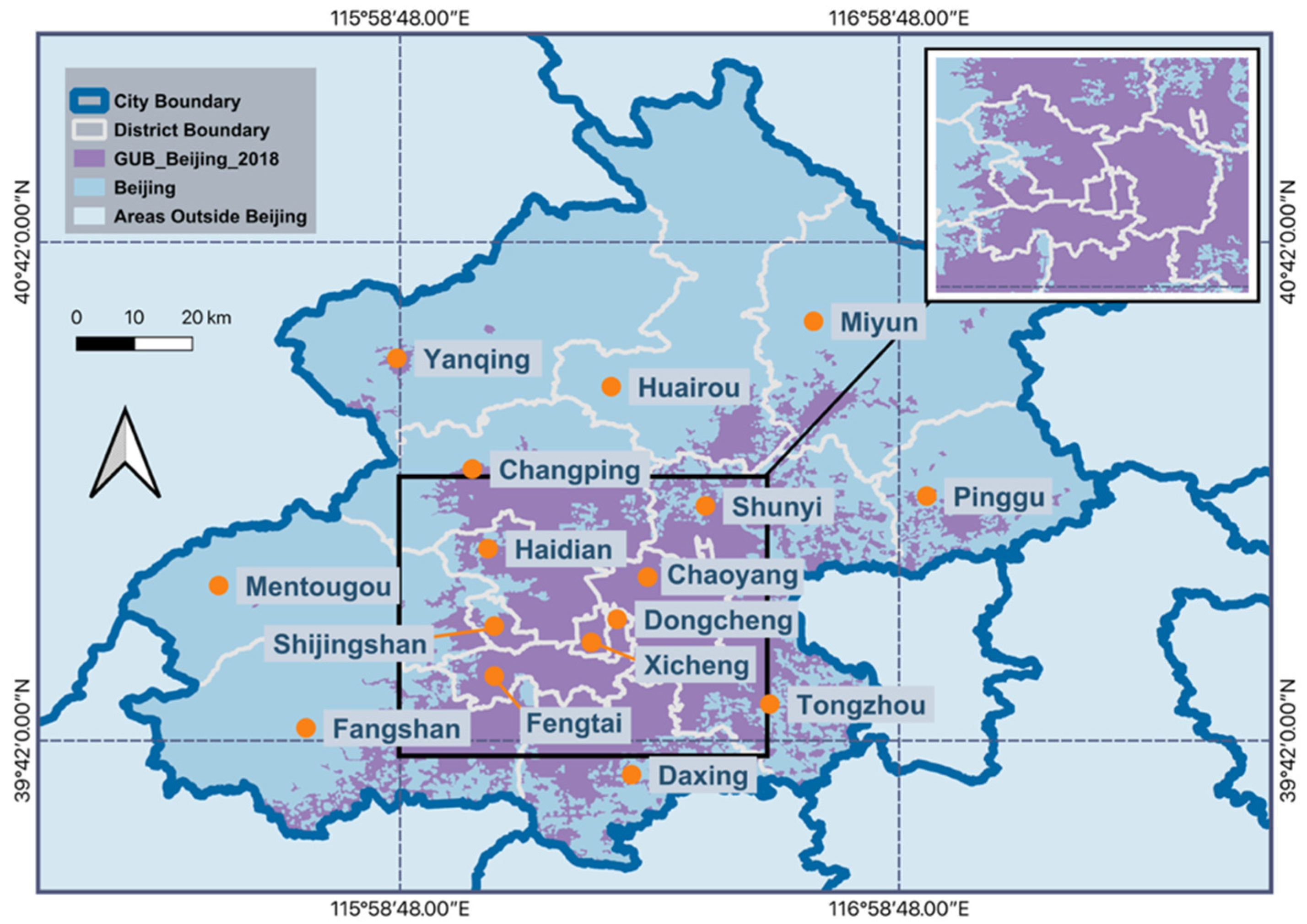
2.1. Study Area

As the capital of China, Beijing is located on the northwestern edge of the North China Plain (Figure 1). Beijing covers a total area of 16,411 km² and has an artificial impervious surface area of 4403 km² [25]. We use the urban area of Beijing, denoted as “GUB_Beijing_2018” in Figure 1, as the study area. Beijing is the political, cultural, educational, technological, and international communication center of China; thus, it is rich in various social media data. Beijing had a resident population of over 21 million in 2019. As one of the most important megacities in China, it is important to study Beijing to understand the ghost city phenomenon in Chinese megacities.

2.2. Datasets

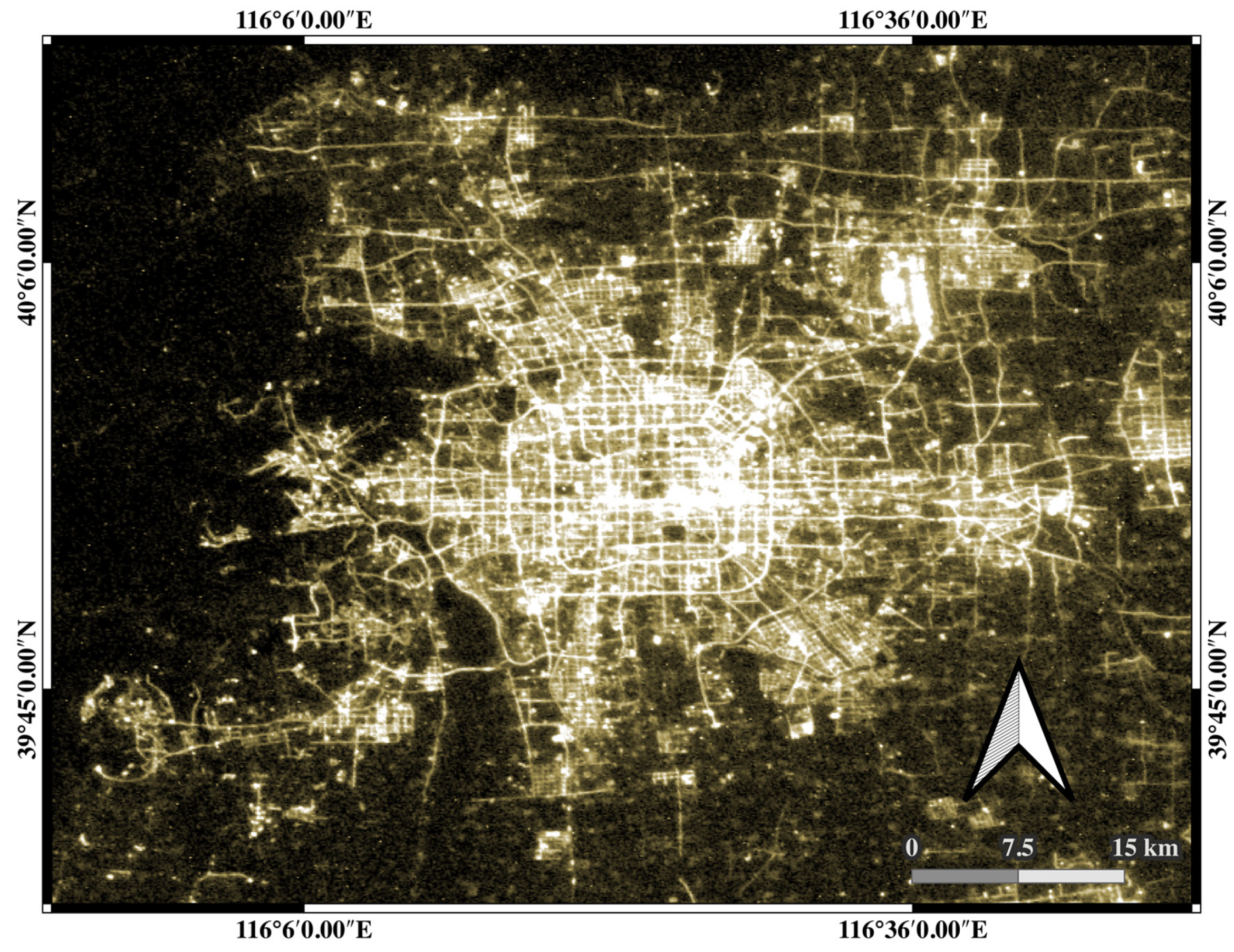
2.2.1. Luojia-1 Nighttime Light Data

The Luojia-1 nighttime light (NTL) data have a ground spatial resolution of 100 to 150 m [26]. Satellite-based remote sensors detect nighttime light emissions from the surface. NTLs reflect the levels of regional development and human activities. The data can be downloaded from the official website of Luojia-1 (http://59.175.109.173:8888/index.html, accessed on 26 June 2020). On June 26, 2020, we downloaded the scene acquired on November 23, 2018, with a resolution of 130 m (http://59.175.109.173:8888/app/single1.html?id=10949, accessed on 26 June 2020) (Figure 2).

2.2.2. Easygo Crowdedness Data

Easygo Crowdedness data are commercial products provided by Tencent. Tencent collects location request data from users’ cell phones to produce these products. With these data, the spatial distribution of relative congestion can be determined in real-time [27]. We obtained the data through the application program interface (http://c.easygo.qq.com/, accessed on 7 September 2019) from 6 September (Friday) to 7 September (Saturday) 2019 at an hourly frequency; however, these data are not currently available. Each record contains information on time, relative congestion level and location coordinates. In this study, Easygo data are used to describe the intensity of human activities at a spatial resolution of 27 m. Figure 3 shows the Easygo crowding data within residential parcels.

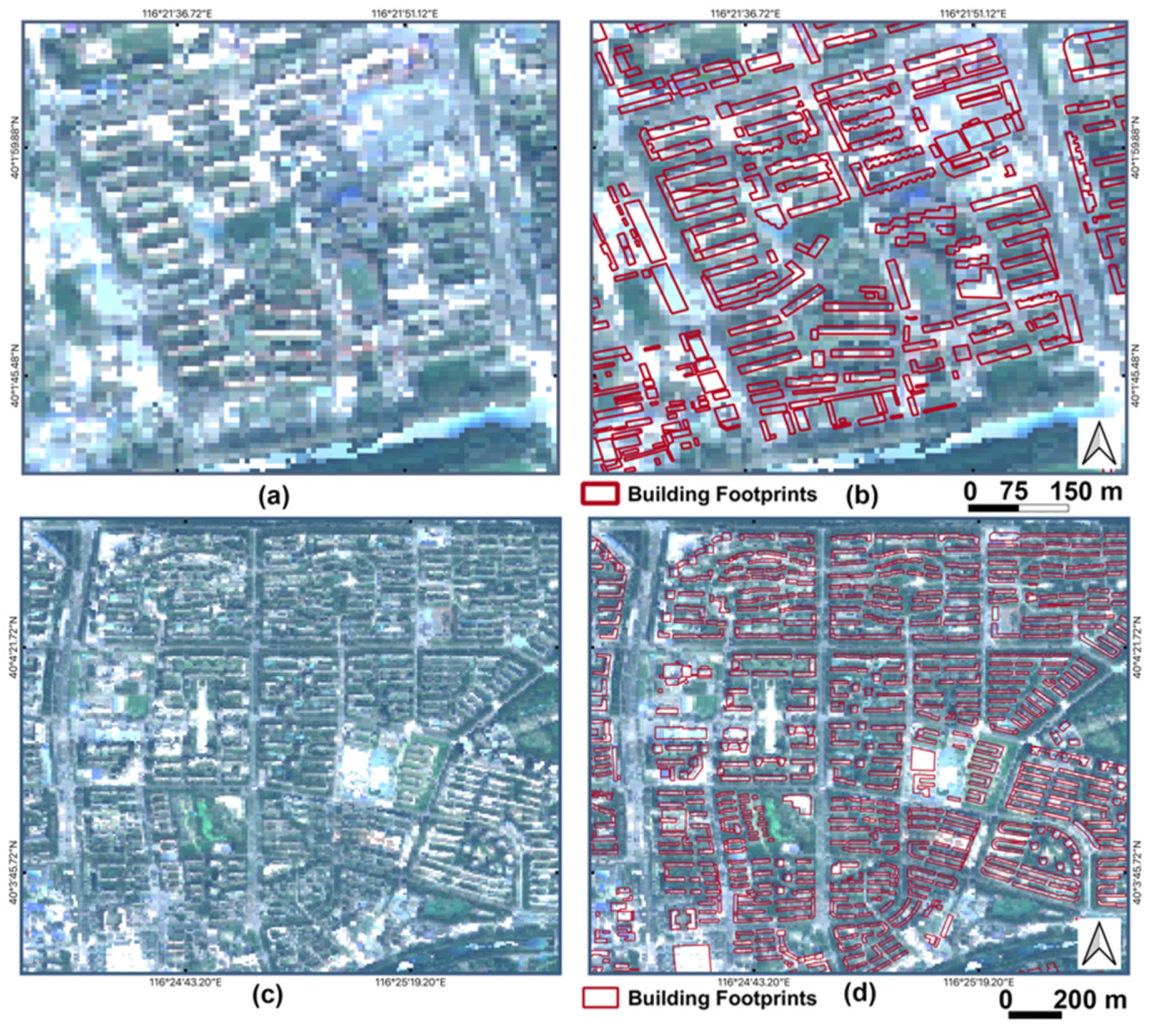
2.2.3. Baidu Maps Building Footprints

Baidu Maps is one of the most popular web mapping platforms in China; it provides a variety of geographic services, such as location search, navigation, and positioning services, to a large number of users. We collected building footprints from Baidu Maps with web crawlers. These building outlines were stored in vector polygon format, and the number of building levels was provided in the attribute information. We used building footprints to determine the building capacity. Figure 4 shows two zoomed-in views of the building footprints used in this study. By comparing Figure 4a,c with Figure 4b,d, respectively, we can find that Baidu Maps building footprint data stored in vector polygon format overlap well with the building contours from optical imagery.

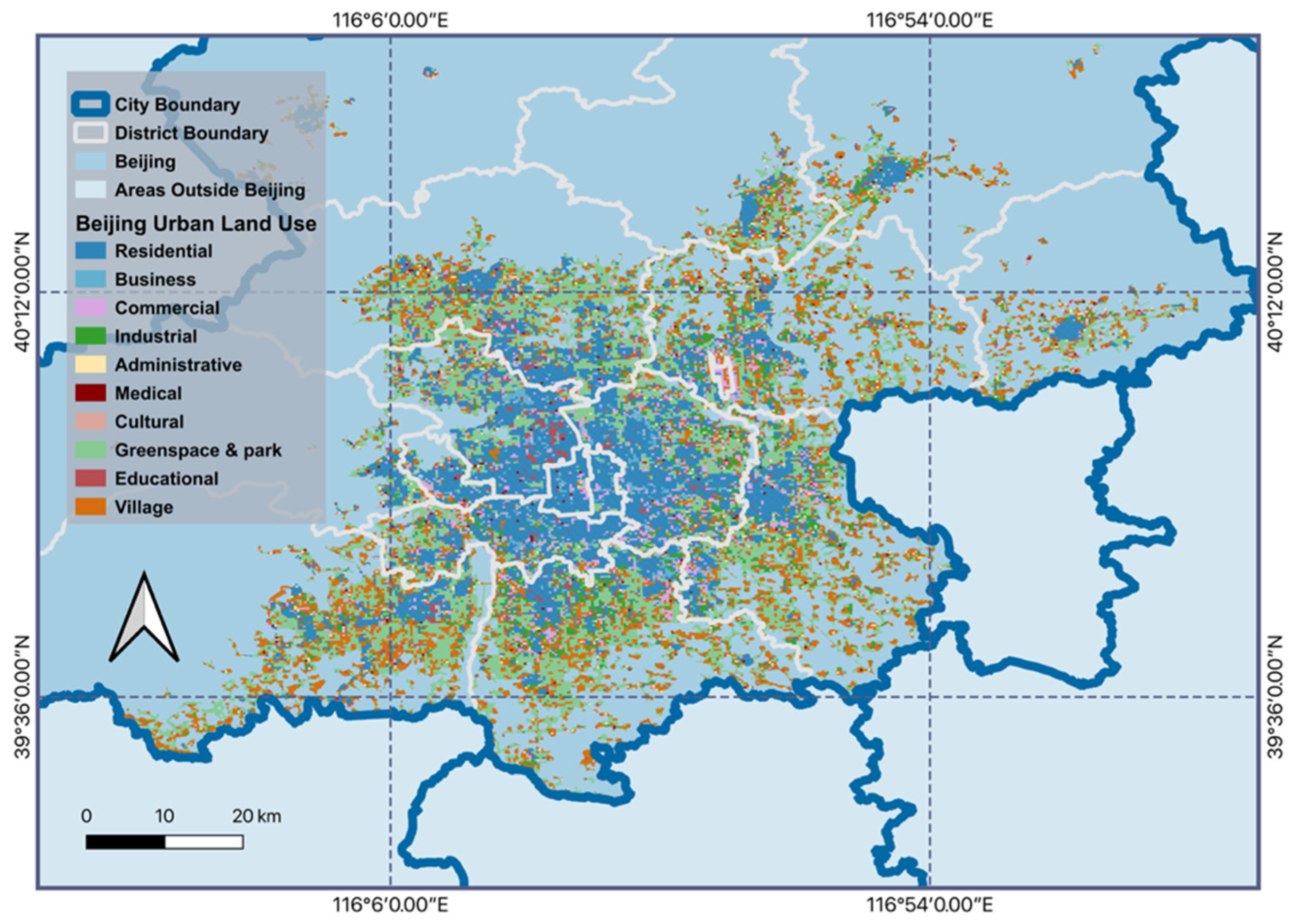
2.2.4. EULUC-Beijing Land Use Product

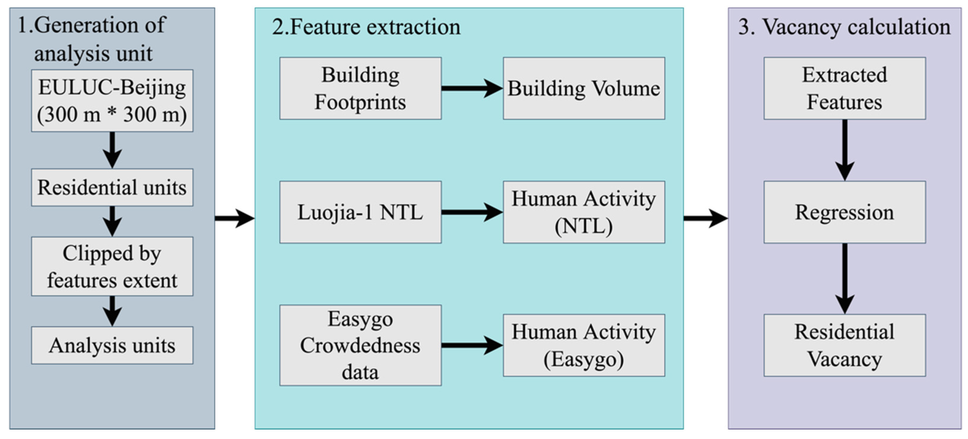
The EULUC-Beijing land use product was produced via the random forest classification method with input features derived from Sentinel-2 optical imagery, Baidu Maps POI and area of interest (AOI) data, Luojia-1 nighttime light imagery, and Easygo crowdedness data. The product consists of 10 categories: residential, business, commercial, industrial, administrative, medical, cultural, greenspace and park, educational, and villages. The product we used was classified to a 300 m × 300 m grid at the unit level before superimposing AOI layers. An overall accuracy of 50% was achieved, with a kappa value of 0.45 at the unit level. We used the residential category, for which a user’s accuracy of 0.68 and a producer’s accuracy of 0.53 [28] was achieved, to refine the study area. Figure 5 illustrates an overview of the EULUC-Beijing land use product.

2.3. Methods

The proposed approach includes three steps (Figure 6). The first step is the generation of analysis units. The second step is feature extraction. The final step is residential vacancy calculation.

2.3.1. Generation of Analysis Units

Easygo crowdedness data are stored in vector point format and distributed over an extent that includes buildings, roads and other features. Such points are difficult to match with polygons at the building scale. To address this issue, 300 m × 300 m residential units from the EULUC-Beijing land use product were selected as study areas. As shown in

Table 1. Extents of datasets.

Data	Extent (Lonmin, Latmin, Lonmax, Latmax)
Residential units	(115.675, 39.447, 117.297, 40.660)
NTL	(113.645, 38.486, 117.506, 41.090)
Easygo	(115.987, 39.653, 116.779, 40.199)
Building footprints	(115.466, 39.491, 117.441, 40.710)

, among the data considered, NTL data have the largest extent, and Easygo crowdedness data have the smallest extent. Therefore, we updated the initially derived research area with an Easygo crowdedness data layer to establish the final research area and analysis units.

2.3.2. Feature Extraction

Extraction of Building Volumes

Building capacity was derived from Baidu Maps building footprints. First, we intersected Baidu Maps building footprints with the analysis units obtained in the first step. We then multiplied the area of a building and the corresponding number of floors to obtain the volume of each building. Then, we summed the volume of each building to obtain the volume in each unit (Equation (1)). Next, we performed min-max normalization (Equation (2)) to prepare for future regression. In this case, a high value represents a large volume and vice versa.

$$Volume={\displaystyle \sum }Area\ast Floors$$

(1)

$$X\_norm=\left(X-Xmin\right)/\left(Xmax-Xmin\right)$$

(2)

Extraction of Human Activity Intensities

Both NTL data and Easygo crowdedness data were used to describe human activity intensities. For the NTL data, we calculated the mean value in each analysis unit. Then, we performed min-max normalization (Equation (2)) to obtain the corresponding human activity intensity. In this case, a high value represents a high level of human activity. In the following paragraphs, we refer to this variable as heat (Luojia).

For the Easygo crowdedness data, we performed some preprocessing steps. The workflow is displayed in Figure 7. The initial data were stored in grid point format at a ground resolution of 27 m. We summed all the crowdedness values at each grid point during 4 p.m. and 10 p.m. when people are mostly at home and have not yet fallen asleep. Then, we summed all the point values within each analysis unit to obtain the total value for the analysis unit. At this step, the Easygo crowdedness data were stored at a spatial resolution of 300 m. Next, we performed min-max normalization (Equation (2)) to obtain human activity intensities. In this case, a high value represents a high level of human activity. We refer to this variable as heat (Easygo).

2.3.3. Vacancy Calculation

We calculated residential vacancies based on heat values (Luojia) derived from the Luojia-1 NTL data, heat values (Easygo) derived from Easygo crowdedness data, and building volumes derived from Baidu Maps building footprints. We designed four different regressions with these features. Specifically, the applied ordinary least squares (OLS) regression methods and the corresponding parameters are listed in

Table 2. OLS regression information. The degree represents the maximum degree of the polynomial features. For example, if an input sample is two dimensional and of the form [a, b], the degree-3 polynomial features are [1, a, b, a², a b, b², a³, a² b, a b², b³]. VLE, VE, VL, LE are the abbreviations corresponding to the methods of each row.

Method	Degree	Independent Variable(s)	Dependent Variable	Abbreviation
nonlinear	3	volume, heat (Luojia)	heat (Easygo)	VLE
linear	1	volume	heat (Easygo)	VE
linear	1	volume	heat (Luojia)	VL
linear	1	heat (Luojia)	heat (Easygo)	LE

. The first approach was third-degree OLS nonlinear regression with volume and heat (Luojia) as independent variables and heat (Easygo) as the dependent variable; this case was abbreviated as VLE. The second approach was OLS linear regression with volume as the independent variable and heat (Easygo) as the dependent variable; this case was abbreviated as VE. The third approach was OLS linear regression with volume as the independent variable and heat (Luojia) as the dependent variable; this case was abbreviated as VL. The fourth approach was OLS linear regression with heat (Luojia) as the independent variable and heat (Easygo) as the dependent variable; this case was abbreviated as LE.

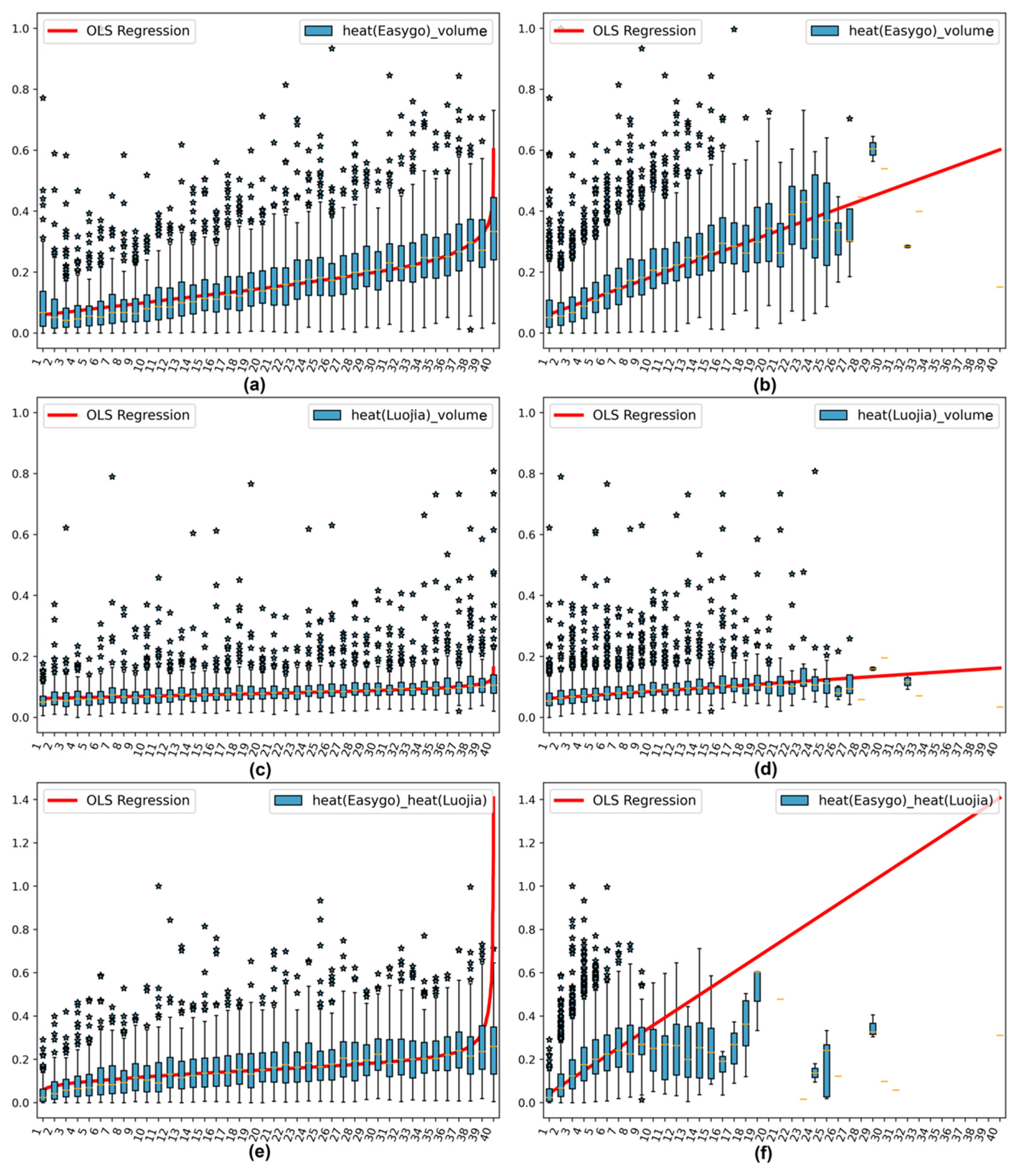
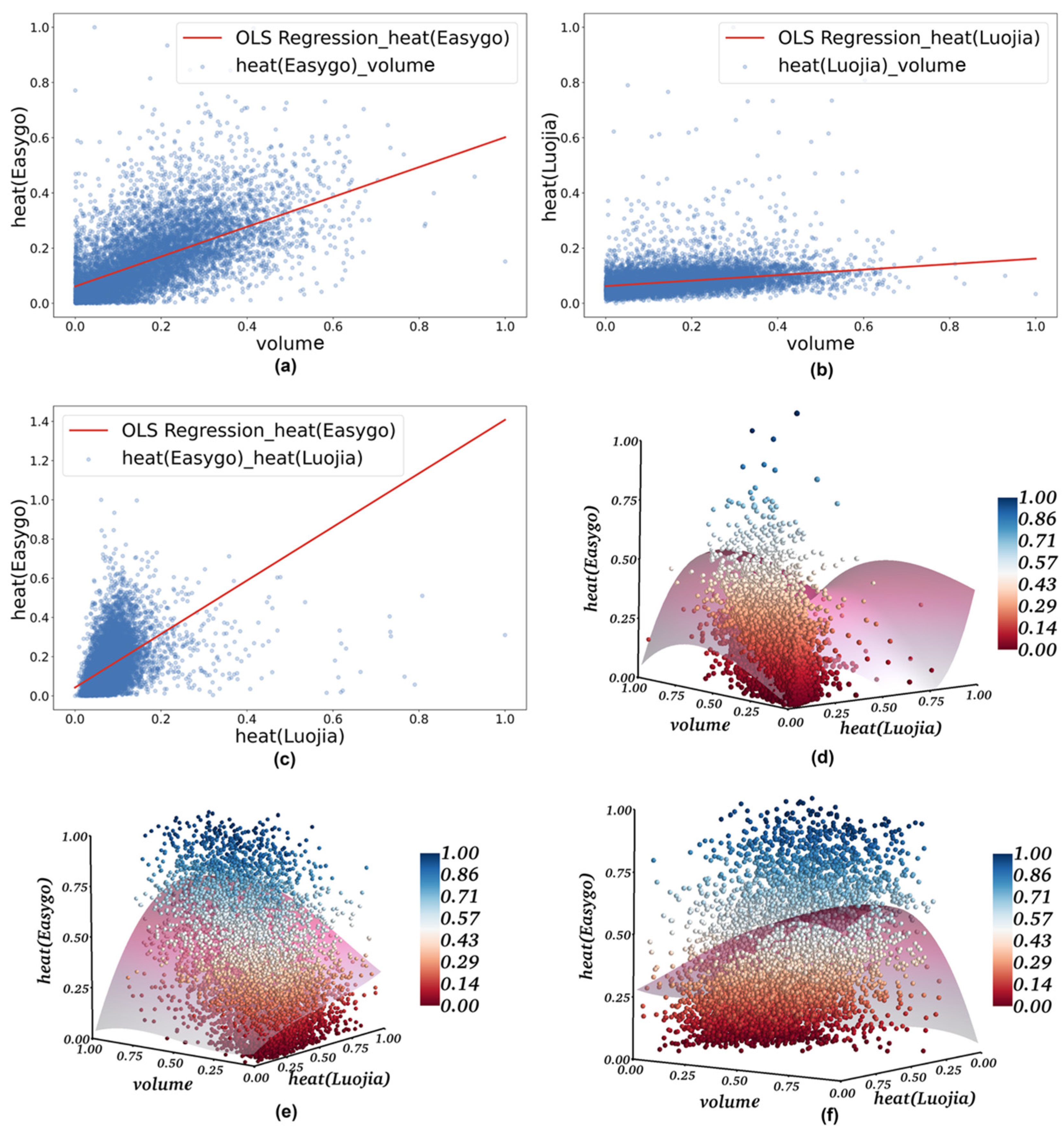
Examination of Features

Before regression analyses were performed, we briefly examined the distribution of feature data. The results are presented in Figure 8. We sorted the features of independent variables in ascending order and divided them into 40 classes with equal counts. Then, we plotted the corresponding features of the dependent variable. Next, we sorted the features of the independent variable in ascending order, divided them into 40 classes with equal intervals and plotted the corresponding features of the dependent variable. We conducted these analyses for VE, VL, and LE listed in Table 2. As shown in Figure 8b,d,f, the data became sparse and oscillatory when the features were sufficiently large. To address this issue, we dropped the largest 5 percent of both independent features and dependent features. Then, we performed regressions with the remaining features (no less than 90.25% of all data). Finally, the regression trends were extended to the whole data range. The OLS linear regression results are illustrated in Figure 8 with red lines, and the trends fit the features well. In addition, there are many high outliers but few low outliers for each OLS linear regression variable pair.

Conducting Regressions

OLS is a linear least-squares method used for estimating unknown parameters in a linear regression model to describe the relationship between one or more independent variables and a dependent variable. This regression approach is used to identify the parameters of explanatory variables based on the principle of least squares: minimizing the sum of squares of differences between the observed dependent variable in the given dataset and the predictions of the regression function of the independent variable.

After the assessments in the previous step, we conducted OLS regressions of the obtained variables. The variable distributions and regression results are displayed in Figure 9. First, we conducted a linear regression for VE. We removed the largest 5 percent of both heat values (Easygo) and volumes and performed regressions with the remaining features. Then, we extended the regression results to the whole data range. The results are displayed in Figure 9a. Next, we repeated the linear regression for VL, and the regression results are displayed in Figure 9b. We also repeated the linear regression for LE, and the results are displayed in Figure 9c.

Finally, we conducted OLS nonlinear regression for VLE. Before dropping the largest 5 percent of variables, we conducted regression with the whole range of data; the corresponding feature distribution and regression results are illustrated in Figure 9d. Notably, the feature data are sparse and oscillatory when all values are considered. Therefore, the regression results fluctuated severely and did not match the actual trend. Then, we repeated the procedure and removed the largest 5 percent of volume, heat (Luojia), and heat (Easygo) values in turn. Then, we performed a regression with the remaining 88.7 percent of the data. Figure 9e,f illustrates the feature distribution and regression results. Next, we extended the regression results to the whole data range to calculate residential vacancies and obtained the corresponding absolute values.

Vacancy Calculation

In previous processing, we obtained the regression heat values corresponding to various building capacities. The regression heat values reflect the general level of the intensity of human activities under each building capacity. Different from the direct calculation of the average value and the median calculation, the regression method makes the intensity of human activities continuous with the change of the building capacity, which is consistent with our cognition. Thus, with the regression results obtained in the previous step, it was simple to calculate the residential vacancy. First, we divided the dependent features based on the corresponding regression results. In other words, for a specific unit, we use the observed human activities intensity to divide the general human activities intensity corresponding to its building capacity to obtain the relative human activity intensity. If the division result is smaller than 1, it means that the human activity intensity of this unit is lower than the general human activity intensity corresponding to the building capacity, which means that the building vacancy is relatively high. If the result is greater than 1, it means that the human activity intensity is greater than the general human activity intensity corresponding to the building capacity, which means that the building occupancy is relatively high, and the building vacancy is relatively low. The smaller the calculated relative human activity intensity value (the result of the division), the more severe the building vacancy. Then, we obtained the quantiles of these divisions for all analysis units. Finally, quantiles were used to determine residential vacancies, varying from 0 to 1, with smaller values indicating a more severe residential vacancy phenomenon.

3. Results

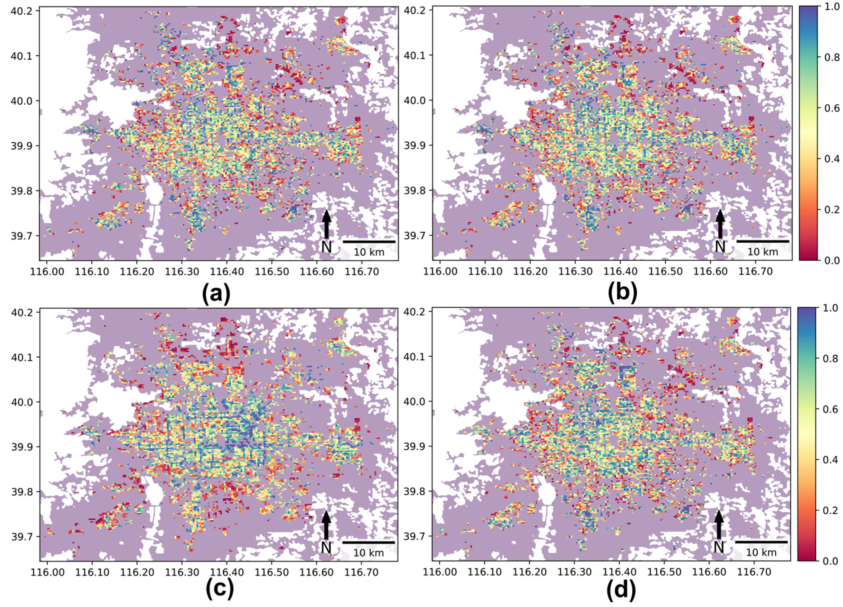
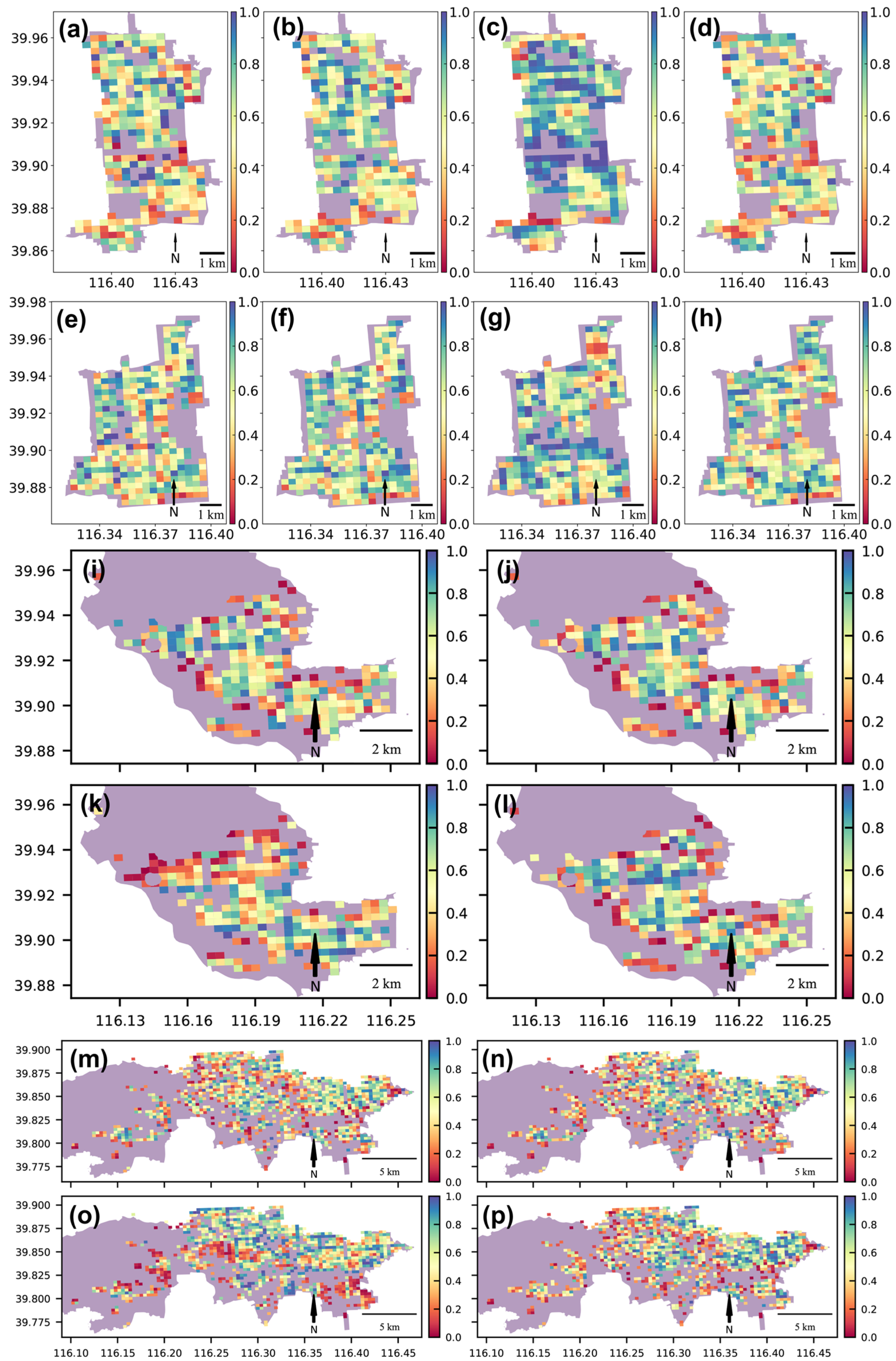
3.1. Spatial Pattern of the Mapping Results

The residential vacancy results are visualized in Figure 10. The OLS nonlinear regression results for VLE are illustrated in Figure 10a. The mapping results for VE, VL, and LE are illustrated in Figure 10b–d, respectively. Figure 10a,b,d are generally similar in terms of spatial distribution, with local differences. In general, urban centers are crowded, and urban fringe areas are comparatively vacant. There is obviously a dense residential vacant area in the northeastern urban fringe region, as shown in Figure 10a,b,d. Small residential areas with low vacancies exist near the coordinate locations of (40.05° N, 116.4° E), (39.75° N, 116.33° E), and (39.77° N, 116.55° E), as shown in Figure 10a,b,d.

Figure 10c is different from the other three figures. The most obvious difference is that in urban centers, there are some low-vacancy clusters. Therefore, we spatially compared the VL mapping results with the main road network. The comparison is illustrated in Figure 11. Figure 11a displays a zoomed-in view of the mapping results, and Figure 11b displays the same zoomed-in view with overlapping main road networks. By comparing Figure 11a with Figure 11b, we find that low-vacancy clusters align well with main roads. This phenomenon was not observed in the other regression results, indicating that road networks might have an impact on ghost city identification based on nighttime light features. This issue should be addressed in future research. Still, the results in Figure 10c highly differed from the mapping results for the other three regression cases. Notably, the low-vacancy clusters around the coordinate locations mentioned above are not present. Additionally, the high-vacancy cluster near (40.05° N, 116.53° E) disappears. In contrast, more high-vacancy clusters can be observed in the southwestern, southern and northwestern urban fringe regions.

3.2. Comparison of Mapping Results at the District Level

We compared the mapping results of the four regressions at the district level. Figure 12 and Figure 13 display the comparison of the results. Figure 12a displays the mapping results for VLE. Figure 12b displays the mapping results for VE. Figure 12c displays the mapping results for VL. Figure 12d displays the mapping results for LE. The following sets of subfigures display the mapping results for Dongcheng, Xicheng, Shijingshan, Fengtai, Haidian, and Chaoyang districts, respectively: Figure 12a–p and Figure 13a–f. Similar to that for the previous results, the spatial pattern of the mapping results for VL, in this case, varied the most from the patterns obtained with the other regression methods in all six districts.

In Figure 12a–d, there are few units with extremely high vacancies. Figure 12a,b,d are similar in some locations. For example, in Figure 12a, b, d, units with relatively high vacancies are scattered around (39.87° N, 116.40° E) and (39.88° N, 116.42° E). In Figure 12a,d, units with relatively high vacancies are also located at approximately (39.90° N, 116.43° E). However, in Figure 12c, the spatial pattern is comparatively different, with most units displaying relatively low vacancy; however, units near (39.87° N 116.41° E) exhibit extremely high vacancy.

Such similarities and differences in spatial patterns can also be observed in other districts. Figure 12e–g show the same clusters with high vacancies near (39.93° N, 116.39° E) and (39.88° N, 116.39° E). Figure 12e shows a high-vacancy cluster at approximately (39.96° N, 116.38° E). Figure 12i,j,l show units with high vacancies along the fringes of residential units in many regions. Figure 12k shows units with high vacancies primarily in the northwestern region. Figure 12m,n,p show units with high vacancies scattered in the center and along the western, southern and eastern fringes. Figure 12o shows clusters with high vacancies in the southwestern and southeastern regions. Figure 13a–d are similar, with high-vacancy units scattered in the northwestern region and units with low vacancy scattered in the southwestern region. Figure 12e,f,h show clusters with extremely high vacancies in the northeastern region and units with relatively high vacancies scattered across the Chaoyang district. Figure 12g shows fewer units with extremely high vacancies than the other figures, and these units are scattered relatively eastward, with clusters of relatively high vacancies in the southern region. Compared with the other three subfigures for the Chaoyang district, Figure 12g displays lower vacancies, with notable low-vacancy clusters in the southwestern region.

3.3. Analysis of the Regression Results

We analyzed the regression results, and they are shown in box plot format in Figure 14. Figure 14a displays the vacancy distribution for VLE in box chart format. Figure 14b–d displays the vacancy distributions for VE, VL, and LE. In Figure 14a, the median and the lower quartile for the Shunyi district are lower than those for other districts, and these values for the Mentougou district are higher than those for other districts. In Figure 14b, the medians for Shunyi and Fangshan districts are lower than those for other districts. The median, lower quartile and upper quartile for the Mentougou district are still higher than those for other districts. In Figure 14c, the median, lower quartile and upper quartile for Shunyi and Fangshan districts are still lower than those for other districts. The median, lower quartile and upper quartile for the Xicheng and Dongcheng districts increased considerably. The values for the Mentougou district remain relatively stable. The results in Figure 14d are similar to those in Figure 14a,b, with the Shunyi district displaying lower values than other districts and the values for the Mentougou district decreasing a little. In addition, the interquartile ranges for the Xicheng and Dongcheng districts are smaller than those for other districts, and the corresponding minimums increased considerably in Figure 14b–d compared with those in Figure 14a. Xicheng and Dongcheng are generally considered the downtown areas of Beijing, and together with the Shijingshan, Chaoyang, Haidian and Fengtai districts, they form the main urban area in the city. The results in Figure 14 highlight this spatial pattern. For example, the median, lower quartile and upper quartile for the Xicheng and Dongcheng districts are relatively high in Figure 14a–d, and the minimum value increases in Figure 14b–d. In addition, the variables for the six main urban districts exhibit high values in the figures, especially in Figure 14c.

We also analyzed the regression results from the aspect of the probability density distribution and illustrate them in Figure 15. We conducted this analysis in Python scripts with “seaborn” library (https://pypi.org/project/seaborn/, accessed on 4 November 2021) at the unit scale of 300 m². We used the “distplot” function (https://seaborn.pydata.org/generated/seaborn.displot.html, accessed on 4 November 2021) and set the “kde” parameter to “True”. Then, a kernel density estimate (KDE) was applied to these vacancy data and the probability density distributions were obtained. Figure 15a displays the probability density distribution for VLE. Figure 15b–d displays the probability density distributions for VE, VL, and LE. Figure 15 provides detailed information regarding the vacancy distribution. Similar to the information obtained from Figure 14, we found that the vacancies for the Xicheng, Dongcheng and Mentougou districts are relatively high. The vacancies for the Chaoyang, Haidian, Fengtai and Tongzhou districts are distributed evenly throughout the data range. The vacancy values in the Shijingshan district are relatively high in Figure 15a,b,d, with a comparatively even distribution in Figure 15c. The vacancies for the Shunyi, Fengtai and Changping districts appear to be relatively low.

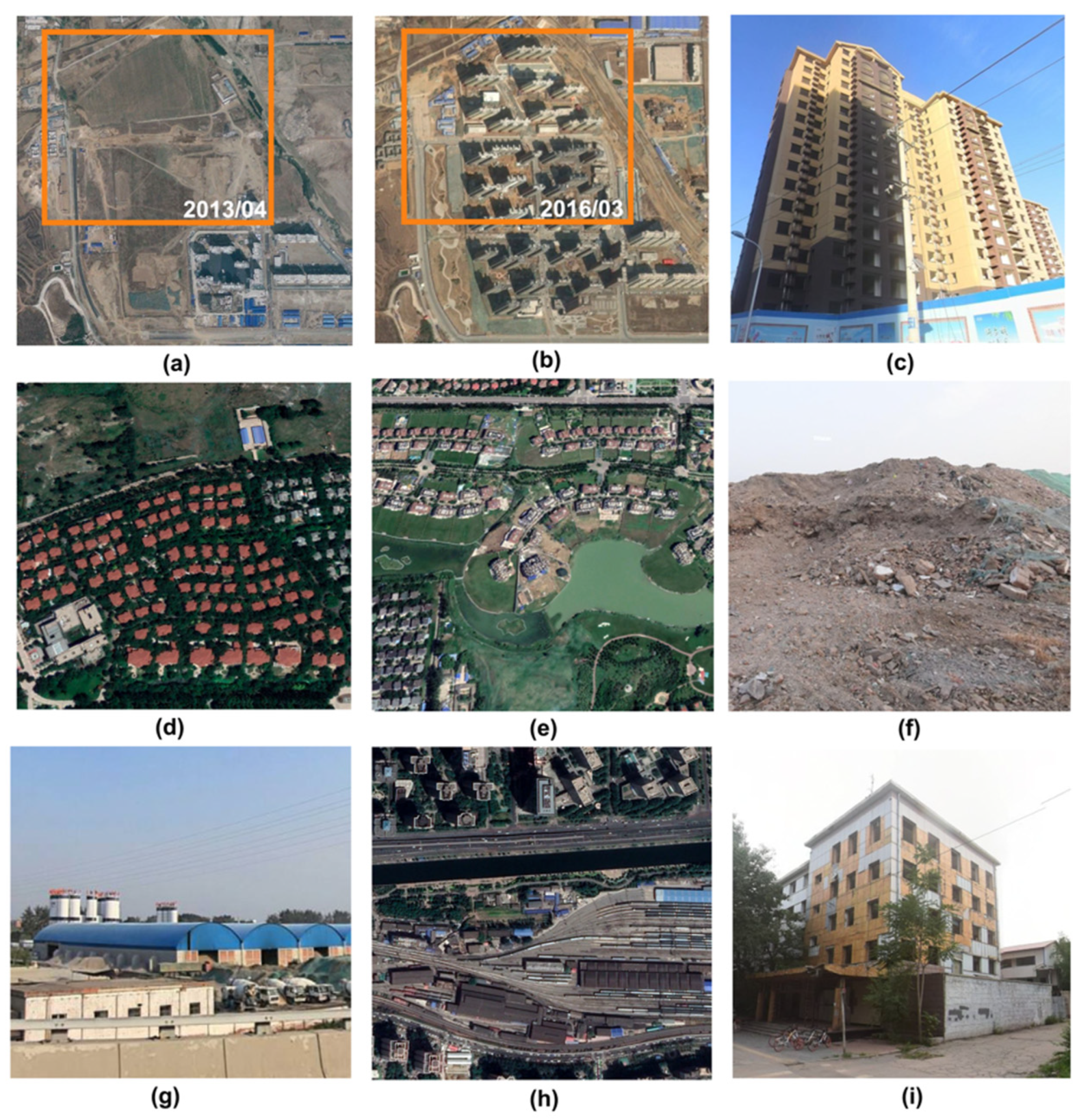
3.4. Validation of the Most-Vacant Units

We manually interpreted the 200 most-vacant units identified with each method through a combination of Google Earth historical imagery and Baidu Maps street view imagery. We categorized the reasons for vacancies and list them in

Table 3. Statistics on the frequency of categorical reasons for vacancies under different methods. In each method, we conducted a manual interpretation of the 200 most vacant units. For example, in the grid of the row where the “VE” is located and the column where the “Villa” is located, the number “96” represents that under the “VE” method, there are 96 units (among 200 units) that are vacant due to “Villa” reason.

Method	Villa	Newly Built	Demolition	Greenspace	Land Use	Wasted	Others
VE	96	22	42	13	19	5	3
LE	48	44	22	50	24	1	11
VL	87	20	40	19	25	5	4
VLE	90	25	39	14	24	5	3

. “Villas” are spacious residences typically designed for wealthy individuals, and they often have prominent green surroundings. As investment homes for the wealthy, villas are often vacant. A “newly built” community may take several years to complete, leading to a lag in population migration and thus vacancies based on the method used in this study. The “demolition” or construction of buildings may cause a delay in the updating of building footprints, resulting in conflicts in vacancy identification. For residential communities surrounded by “greenspaces”, lower nighttime light levels resulted in the identification of vacancies. “Land use” classification errors can also lead to vacancy identification issues. For example, an educational community or industrial community can be vacant after working hours. The “wasted” land use class includes neighborhoods that are nearly completely vacant, and “others” include nonvacant communities without other information available. We attributed the findings in each unit to a certain reason, but these patterns may be influenced by multiple factors. For example, villas are usually surrounded by rich vegetation, and the corresponding trend can thus be associated with both the villa and greenspace categories. In addition, the most active areas where new communities are constructed are in suburban regions. Thus, vacancies in a suburban community could be associated with villas, newly built areas, demolition, greenspaces, land use, wasted areas and others.

Table 3 shows that villas are common in vacant communities in Beijing, with 96, 48, 87, and 90 cases observed for VE, LE, VL, and VLE, respectively. Greenspaces have a notable influence on the building footprint results, with 13, 19, and 14 cases noted for VE, VL, and VLE, respectively, and 50 cases for LE. Mainly occurring in suburban areas, the active transformation of the land surface, such as through demolition and construction (newly built), also contributes to temporary vacancies in Beijing, with 64, 66, 60 and 64 cases for VE, LE, VL, and VLE, respectively. In megacities, such as Beijing, totally wasted communities are uncommon, with five, one, five and five cases for VE, LE, VL, and VLE, respectively.

Some sample communities are displayed in Figure 16. Figure 16a,b show images of communities under construction. Figure 16c shows a newly built community that has not yet been populated. Figure 16d shows villas, and Figure 16e shows a community surrounded by rich vegetation. Figure 16f shows an example of a demolition area. Figure 16g–h show two sample locations of land use confusion. Figure 16i displays an example of a wasted community.

3.5. Discussion of Advantages and Disadvantages among Methods

After analysis and manual interpretation of validation units, we find some advantages and disadvantages among these four methods. From Table 3 we noticed that the LE method is insufficient when identifying vacancies resulting from villas, and it overidentified vacancies where buildings are surrounded by prominent greenspace. The VE, VL, and VLE methods identified similar results from the validation results displayed in Table 3. Comparing the mapping results of the VL method and the corresponding road network in Figure 11, we found that the mapping results of the VL method were seriously affected by the nighttime lights of road networks. The mapping results and analysis results of the VE and VLE methods appear to be similar to each other, and they are less affected by green spaces and road lights, which are more appropriate. The VLE method comprehensively utilizes building capacity, nighttime light intensity, and Easygo crowdedness information to identify residential vacancies. However, the VLE method is restricted by the spatial resolution of the nighttime light data. The building footprints and Easygo crowdedness data have a finer spatial resolution. Thus, when there is a lack of nighttime light data or residential vacancies are explored at a higher spatial resolution, the VE method is recommended.

4. Discussion

In this paper, an unsupervised approach for residential vacancy assessment based on multisource spatiotemporal data is proposed for Beijing, the capital of China. Residential vacancies are derived from high-resolution data sources via a regression function. With these high-resolution data, this approach captures detailed spatial patterns and provides valuable spatial information. Such widespread social media and satellite imagery data sources add to the consistency of residential vacancy identification across China, and vacancy trends among different cities can be compared. In addition, this approach requires no prior knowledge or complicated user-defined indicators, making it easily applicable to cities across China at a fine resolution.

However, there are limitations in our research that must be improved in future works. Different land use types are associated with different patterns of human activities. Thus, accurate and reliable land use products are critical when analyzing residential vacancies. Efforts to improve land use products should be addressed.

Nighttime imagery, which has been widely used in previous studies, is greatly affected by the road network, which may lead to misleading human activity trends in communities, areas with many roads in urban centers and areas with buildings surrounded by abundant vegetation in the urban fringe regions. Therefore, it is necessary to preprocess nighttime light imagery and road information. In addition, the underestimation of human activities in suburban regions should be addressed.

The consistency and availability of building footprints downloaded from web maps are not as good as those for information obtained through optical images. In fast-growing cities, such as Beijing, the land surface is actively changing, especially in the suburbs. Demolition and construction occur in many areas. Building footprints from web maps are gradually established over a period of time. Due to technical limitations and cost considerations, commercial companies may not perform real-time updates. In addition, the quality of data in suburban areas is often unsatisfactory. Inconsistent acquisition times, outdated data and other issues will reduce the accuracy of residential vacancy identification. Therefore, efficiently and accurately extracting building footprints from high-resolution remote sensing imagery is an important task.

In addition to these issues regarding data quality, time series analysis may be necessary for ghost neighborhood research. In fast-growing countries, building footprints are rapidly changing, and the population is continually migrating in China. Therefore, time series analysis is needed to determine whether buildings are currently in a stable state, under construction, or under demolition. For buildings under construction or being demolished, a low level of human activity is normal. Additionally, it may take several years before residents or workers migrate to newly constructed buildings.

5. Conclusions

In this study, we mapped residential vacancies in Beijing via a regression function with Easygo crowdedness data, Luojia-1 nighttime imagery and Baidu Maps building footprint data as regression features. We took the predicted values of the regression function as the standard heat values of analysis units. Next, we divided each unit by the corresponding standard heat value. Then, we obtained the quantiles of these division results for all analysis units. Finally, quantiles were used to determine residential vacancy levels, varying from 0 to 1. With these high-resolution data sources, the mapping results provide detailed spatial information at a 300 m × 300 m scale. This approach is widely applicable, making residential vacancy results comparable among different cities in China. Moreover, this approach requires no prior knowledge or complicated user-defined indicators and can be easily applied across cities in China.

References

1. Li, H.; Wei, Y.D.; Liao, F.H.; Huang, Z. Administrative hierarchy and urban land expansion in transitional China. Appl. Geogr. 2015, 56, 177–186. [Google Scholar] [CrossRef]
2. Wang, L.; Li, C.; Ying, Q.; Cheng, X.; Wang, X.; Li, X.; Hu, L.; Liang, L.; Yu, L.; Huang, H.; et al. China’s urban expansion from 1990 to 2010 determined with satellite remote sensing. Chin. Sci. Bull. 2012, 57, 2802–2812. [Google Scholar] [CrossRef] [Green Version]
3. Gong, P.; Li, X.; Zhang, W. 40-Year (1978–2017) human settlement changes in China reflected by impervious surfaces from satellite remote sensing. Sci. Bull. 2019, 64, 756–763. [Google Scholar] [CrossRef] [Green Version]
4. Cartier, C. Territorial Urbanization and the Party-State in China. Territ. Politics Gov. 2015, 3, 294–320. [Google Scholar] [CrossRef]
5. Gu, C.; Wei, Y.D.; Cook, I.G. Planning Beijing: Socialist city, transitional city, and global city. Urban Geogr. 2015, 36, 905–926. [Google Scholar] [CrossRef]
6. Lu, H.; Zhang, C.; Liu, G.; Ye, X.; Miao, C. Mapping China’s Ghost Cities through the Combination of Nighttime Satellite Data and Daytime Satellite Data. Remote Sens. 2018, 10, 1037. [Google Scholar] [CrossRef] [Green Version]
7. Young, O.R.; Guttman, D.; Qi, Y.; Bachus, K.; Belis, D.; Cheng, H.; Lin, A.; Schreifels, J.; Van Eynde, S.; Wang, Y.; et al. Institutionalized governance processes: Comparing environmental problem solving in China and the United States. Glob. Environ. Chang. 2015, 31, 163–173. [Google Scholar] [CrossRef]
8. Shepard, W. Ghost Cities of China: The Story of Cities without People in the World’s most Populated Country, 1st ed.; Zed Books: London, UK, 2015; p. 218. [Google Scholar]
9. Chen, Z.; Yu, B.; Hu, Y.; Huang, C.; Shi, K.; Wu, J. Estimating House Vacancy Rate in Metropolitan Areas Using NPP-VIIRS Nighttime Light Composite Data. IEEE J. Sel. Top. Appl. Earth Obs. Remote Sens. 2015, 8, 2188–2197. [Google Scholar] [CrossRef]
10. Zheng, Q.; Zeng, Y.; Deng, J.; Wang, K.; Jiang, R.; Ye, Z. “Ghost cities” identification using multi-source remote sensing datasets: A case study in Yangtze River Delta. Appl. Geogr. 2017, 80, 112–121. [Google Scholar] [CrossRef]
11. Guidance from the Ministry of Land and Resources on Promoting the Economical and Intensive Use of Land. Available online: http://f.mnr.gov.cn/202102/t20210214_2611863.html (accessed on 29 June 2020).
12. Chi, G.; Liu, Y.; Wu, H.J.A. Ghost Cities Analysis Based on Positioning Data in China. arXiv 2015, arXiv:1510.08505. [Google Scholar]
13. Leichtle, T.; Lakes, T.; Zhu, X.X.; Taubenböck, H. Has Dongying developed to a ghost city?—Evidence from multi-temporal population estimation based on VHR remote sensing and census counts. Comput. Environ. Urban Syst. 2019, 78, 101372. [Google Scholar] [CrossRef]
14. Deng, J.S.; Wang, K.; Hong, Y.; Qi, J.G. Spatio-temporal dynamics and evolution of land use change and landscape pattern in response to rapid urbanization. Landsc. Urban Plan. 2009, 92, 187–198. [Google Scholar] [CrossRef]
15. Xie, Y.; Weng, Q. Updating urban extents with nighttime light imagery by using an object-based thresholding method. Remote Sens. Environ. 2016, 187, 1–13. [Google Scholar] [CrossRef]
16. Gao, B.; Huang, Q.; He, C.; Sun, Z.; Zhang, D. How does sprawl differ across cities in China? A multi-scale investigation using nighttime light and census data. Landsc. Urban Plan. 2016, 148, 89–98. [Google Scholar] [CrossRef]
17. Yu, B.; Shi, K.; Hu, Y.; Huang, C.; Chen, Z.; Wu, J. Poverty Evaluation Using NPP-VIIRS Nighttime Light Composite Data at the County Level in China. IEEE J. Sel. Top. Appl. Earth Obs. Remote Sens. 2015, 8, 1217–1229. [Google Scholar] [CrossRef]
18. Cai, J.; Huang, B.; Song, Y. Using multi-source geospatial big data to identify the structure of polycentric cities. Remote Sens. Environ. 2017, 202, 210–221. [Google Scholar] [CrossRef]
19. Zhang, Q.; Seto, K.C. Mapping urbanization dynamics at regional and global scales using multi-temporal DMSP/OLS nighttime light data. Remote Sens. Environ. 2011, 115, 2320–2329. [Google Scholar] [CrossRef]
20. Zheng, Q.; Deng, J.; Jiang, R.; Wang, K.; Xue, X.; Lin, Y.; Huang, Z.; Shen, Z.; Li, J.; Shahtahmassebi, A.R. Monitoring and assessing “ghost cities” in Northeast China from the view of nighttime light remote sensing data. Habitat Int. 2017, 70, 34–42. [Google Scholar] [CrossRef]
21. Ju, Y.; Dronova, I.; Ma, Q.; Zhang, X. Analysis of urbanization dynamics in mainland China using pixel-based night-time light trajectories from 1992 to 2013. Int. J. Remote Sens. 2017, 38, 6047–6072. [Google Scholar] [CrossRef]
22. Ge, W.; Yang, H.; Zhu, X.; Ma, M.; Yang, Y. Ghost City Extraction and Rate Estimation in China Based on NPP-VIIRS Night-Time Light Data. Isprs Int. J. Geo-Inf. 2018, 7, 219. [Google Scholar] [CrossRef] [Green Version]
23. Jin, X.; Long, Y.; Sun, W.; Lu, Y.; Yang, X.; Tang, J. Evaluating cities’ vitality and identifying ghost cities in China with emerging geographical data. Cities 2017, 63, 98–109. [Google Scholar] [CrossRef]
24. Williams, S.; Xu, W.; Tan, S.B.; Foster, M.J.; Chen, C. Ghost cities of China: Identifying urban vacancy through social media data. Cities 2019, 94, 275–285. [Google Scholar] [CrossRef]
25. Gong, P.; Li, X.; Wang, J.; Bai, Y.; Chen, B.; Hu, T.; Liu, X.; Xu, B.; Yang, J.; Zhang, W.; et al. Annual maps of global artificial impervious area (GAIA) between 1985 and 2018. Remote Sens. Environ. 2020, 236, 111510. [Google Scholar] [CrossRef]
26. Li, X.; Zhao, L.; Li, D.; Xu, H. Mapping Urban Extent Using Luojia 1-01 Nighttime Light Imagery. Sensors 2018, 18, 3665. [Google Scholar] [CrossRef] [PubMed] [Green Version]
27. Li, F.; Zhang, F.; Li, X.; Wang, P.; Liang, J.; Mei, Y.; Cheng, W.; Qian, Y. Spatiotemporal Patterns of the Use of Urban Green Spaces and External Factors Contributing to Their Use in Central Beijing. Int. J. Environ. Res. Public Health 2017, 14, 237. [Google Scholar] [CrossRef]
28. Li, X.; Hu, T.; Gong, P.; Du, S.; Chen, B.; Li, X.; Dai, Q. Mapping Essential Urban Land Use Categories in Beijing with a Fast Area of Interest (AOI)-Based Method. Remote Sens. 2021, 13, 477. [Google Scholar] [CrossRef]
Figure 1. Map of the study area.
Remotesensing 14 00376 g001
Figure 2. Luojia-1 NTL product used in this study.
Remotesensing 14 00376 g002
Figure 3. Easygo data used in this study.
Remotesensing 14 00376 g003
Figure 4. Zoomed-in views of Baidu Maps building footprints. (a,c) Optical images without building footprints. (b,d) Optical images with building footprints.
Remotesensing 14 00376 g004
Figure 5. Overview of the EULUC-Beijing land use product.
Remotesensing 14 00376 g005
Figure 6. Workflow of residential vacancy calculations.
Remotesensing 14 00376 g006
Figure 7. Workflow of Easygo crowdedness data processing.
Remotesensing 14 00376 g007
Figure 8. Results of the assessments of regression variables. (a) Equal-count split for VE. (b) Equal-interval split for VE. (c) Equal-count split for VL. (d) Equal-interval split for VL. (e) Equal-count split for LE. (f) Equal-interval split for LE.
Remotesensing 14 00376 g008
Figure 9. Feature distribution and regression results. (a) Feature distribution and regression results for VE. (b) Feature distribution and regression results for VL. (c) Feature distribution and regression results for LE. (d) Feature distribution for the whole range and the regression results for VLE. (e,f) Feature distribution after selection and the regression results for VLE.
Remotesensing 14 00376 g009
Figure 10. Mapping results for residential vacancy. (a) Mapping result for VLE. (b) Mapping result for VE. (c) Mapping result for VL. (d) Mapping result for LE.
Remotesensing 14 00376 g010
Figure 11. Comparison of the regression mapping results and the road network. (a) A zoomed-in view of the OLS linear regression results for VL. (b) The same view as (a) with the road network overlaid.
Remotesensing 14 00376 g011
Figure 12. Comparison of the mapping results of the four regressions at the district level. (a) Mapping results for VLE in Dongcheng district. (bd) Mapping results for VE, VL, and LE in Dongcheng district. (ep) Mapping results for Xicheng, Shijingshan and Fengtai districts (in the same order as (ad)).
Remotesensing 14 00376 g012
Figure 13. Comparison of the mapping results for VLE, VE, EL, LE at the district level. (ah) Mapping results for Haidian and Chaoyang districts (in the same order as Figure 12a–d).
Remotesensing 14 00376 g013
Figure 14. Box plots of the vacancy distribution at the district level. (a) Box plot of the vacancy distribution for VLE. (bd) Box plots of the vacancy distributions for VE, VL, and LE.
Remotesensing 14 00376 g014
Figure 15. Probability density distributions of regressions. (a) Probability density distribution for VLE. (bd) Probability density distributions for VE, VL, and LE.
Remotesensing 14 00376 g015
Figure 16. Validation of samples. (a,b) Communities under construction. (c) Newly built community (d) Villas. (e) Communities surrounded by rich vegetation. (f) Demolition. (g,h) Land use conflict. (i) Wasted community.
Remotesensing 14 00376 g016