Noise Removal and Feature Extraction in Airborne Radar Sounding Data of Ice Sheets

Abstract

The airborne ice-penetrating radar (IPR) is an effective method used for ice sheet exploration and is widely applied for detecting the internal structures of ice sheets and for understanding the mechanism of ice flow and the characteristics of the bottom of ice sheets. However, because of the ambient influence and the limitations of the instruments, IPR data are frequently overlaid with noise and interference, which further impedes the extraction of layer features and the interpretation of the physical characteristics of the ice sheet. In this paper, we first applied conventional filtering methods to remove the feature noise and interference in IPR data. Furthermore, machine learning methods were introduced in IPR data processing for noise removal and feature extraction. Inspired by a comparison of the filtering methods and machine learning methods, we propose a fusion method combining both filtering methods and machine-learning-based methods to optimize the feature extraction in IPR data. Field data tests indicated that, under different conditions of IPR data, the application of different methods and strategies can improve the layer feature extraction.

1. Introduction

Due to global warming, the ice mass loss of polar ice sheets in Greenland and Antarctica is increasing [1]. The polar ice sheet is believed to be losing mass at a progressively increasing rate throughout the 21st Century and beyond, and in the case of high greenhouse gas emissions, the rate and amplitude of the ice loss are expected to further increase in the second half of the 21st Century [2]. Recent studies agree that the acceleration of the ice flow in Antarctica has been observed in the Amundsen Sea sector in the West Antarctic ice sheet and Wilkes Land in the East Antarctic ice sheet, which has the potential to lead to a sea level rise by several meters in a few centuries and may imply the beginning of marine ice sheet instability [3,4,5]. Therefore, the measurement and monitoring of ice sheets are essential to evaluate the instability of these ice sheets and their contribution and uncertainty to future sea level rise. At present, the uncertainties in ice sheet instability are mainly related to inadequate observations; an insufficient representation of the mechanical process in ice sheet models; and a limited understanding of the complex interaction among the atmosphere, the ocean, and the ice sheet [2]. Fortunately, the internal stratigraphy of the ice sheet provides important climate achives and ice dynamics [6,7,8]. The geometry, ice thickness, and rheological properties of the ice shelf are also key factors restricting the stress balance of the ice shelf model, which is critical for grounding zones to understand the interaction between coastal ice and the ocean [9,10].

As an efficient and high-resolution geophysical approach, ground-based and airborne radar sounding has been mainly applied to measure the ice thickness, the subglacial topography, and the englacial structure of the polar ice sheets in a wide range since the 1960s [11,12,13]. At present, these radar data are extensively used to characterize the basal conditions of ice sheets [14,15] and to provide constraints in the extrapolation of englacial structures and processes [6,16,17]. Radar data are also used to evaluate ice flow dynamics [18,19], to calculate the basal roughness [20,21], to estimate heat flux and englacial temperature [22,23], to calculate basal reflectivity, and thus, to reveal subglacial lakes and hydrological drainages [24,25].

However, radar-sounding data are inevitably mixed with interference and noise, which seriously hinder the interpretation of the ice sheet characteristics [26]. In order to better use radar data to understand the dynamic process of ice sheets, data processing is a necessary first step to improving the signal-to-noise ratio (SNR) and accurately extracting parametric features. At present, filtering and noise reduction in radar data have become essential processing steps [27,28]. One method of processing the radar waveform is to form an image in which the variance of strong scattering points is extracted as the input feature. Before image-based target classification, preprocessing the image is necessary, such as image denoising and edge feature extraction. Short-time Fourier transform (STFT) [29], empirical mode decomposition (EMD) [30,31], and two-dimensional variation mode decomposition (2D-VMD) [32,33,34] have been used for denoising and edge feature extraction. However, the limitation of filtering technology is the risk of over-processing, that is, it both effectively filters the noise and weakens the effective signal simultaneously.

Another innovative field of data processing is automatic methods used to interpret ice radar images, which is a prerequisite for the effective use of information content from large-volume datasets [13]. At present, automatic algorithms are mainly used in ice surface, bed and internal layer tracking, and basic feature classification [35,36,37,38]. Castelletti and others [39] recently proposed a recognition method that can distinguish clutter using the cross-channel interference phase difference, but this is only effective for surface cross-orbit clutter. Xiong and others [35] used a continuous wavelet transform (CWT) to automatically detect radar echo peaks. They developed a Ricker or Morlet wavelet combined with the Hough transform to extract the englacial layers. Delf and others [40] found that the results of Xiong and others [35] can suppress noise in high amplitudes of the ice layers, but failed to successfully pick up the layers in the low-amplitude area. Machine-learning-based interpretation methods have been widely developed in recent years [41]. Deep neural networks, which when supervised, learn from the manual-picked label, were applied in the automatic tracing of the bedrock interface [42], the internal layer [38], and the snow layer [43]. The unsupervised learning method the cycle generative adversarial network (CycleGAN) has been applied in the removal of interference and in highlighting the layers [44]. Due to a lack of ground truth labeling, the accuracy of CycleGANs in layer extraction is limited. Recently, EisNet [45] introduced a novel approach for extracting the internal ice layer and bedrock interface simultaneously. EisNet was trained on synthetic radar images and labels, and hence could avoid specific noise and interference by appending the visually similar noise in the synthetic dataset for training. Due to the complexity of noise and interference, it is still hard to automatically achieve perfect results in layer tracing by a single filtering method or neural network.

In this article, we focus on the methods applied in the Chinese National Antarctic Research Expedition (CHINARE) data for noise removal and feature extraction. First, the filtering methods, as a representation of conventional methods, are described and tested on two lines of field data from CHINARE data to demonstrate the removal of specific noise and interference. Second, we introduce and apply machine learning methods, including dictionary learning and neural networks, for the tasks of both noise removal and layer feature extraction. Slices from CHINARE were applied in the testing of the methods. Lastly, we propose combined applications of both conventional methods and a machine learning method to remove noise and to enhance the layer feature extraction.

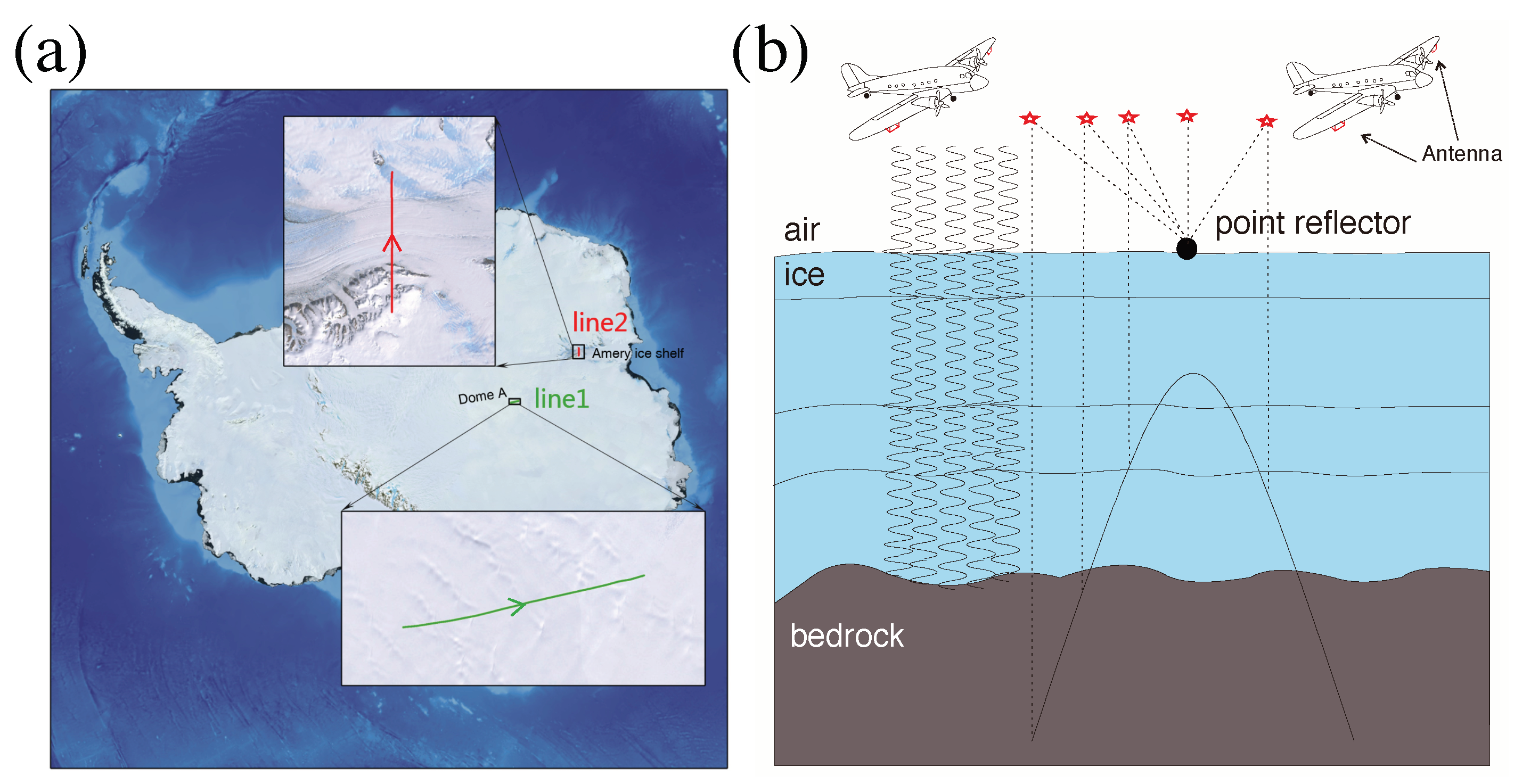
2. Data and Filtering Method

Since 2015, the Snow Eagle 601 fixed-wing airborne platform has performed Antarctic airborne geophysical surveys in five seasons by CHINARE, including IPR, gravity, magnetic, GPS, and optical and laser surface altimetry measurements. It covers several critical areas in East Antarctica, such as Princess Elizabeth Land, Ridge B, the Amery ice shelf, the West ice shelf, the Shackleton ice shelf, the George V coast, and the David Glacier catchment. The IPR, also named the High-Capability Airborne Radar Sounder (HiCARS), is a phase coherent radar system developed by the University of Texas Institute for Geophysics (UTIG), which has been used for measuring englacial stratigraphy, subglacial topography, and ice thickness [46,47,48,49]. HiCARS transmits 1 $\mathsf{\mu }$s-wide VHF chirps, linearly sweeping the frequency between $52.5$ MHz and $67.5$ MHz, with a 60 MHz center frequency, 15 MHz bandwidth, and 8 kW peak transmit power. The pulse repetition frequency is 6250 Hz, with 32 stacking traces in the hardware and a “slow time” sampling rate of 196 Hz for the trace dimension. The received signals are digitized with a 50 MHz sampling rate for a sampling time window of 64 $\mathsf{\mu }$s. Two flat-plate dipole antennas installed under the wings are used for both transmitting and receiving and provide a total bidirectional gain of 18 dB (Figure 1). The system has two channels with low gain for the surface and higher gain for the bed. Raw IPR data are processed through down-conversion, removing direct current offsets, pulse compression, filtering, coherent stacking ten times, and incoherent stacking five times to generate a field data product, referred to as “pik1”. The unfocused coherent stack in pik1 processing improves the SNR of horizontal internal reflectors and reduces surface scattering, but can eliminate inclined reflectors, while the incoherent stack retains steep reflectors, but loses some geometric fidelity [48,50]. The along-track horizontal sampling rate of the pik1 data is ∼20 m and the vertical resolution is ∼5.6 m [51].

2.1. F–K and KL Filtering

We selected two lines of typical radar data, as shown in Figure 1. We first used matGPR (ground penetrating radar (GPR)) software based on MATLAB to further process the pik1 data to improve the SNR [52]. The processing applied by traditional methods involved time zero correction, the Karhunen–Loeve (KL) filter [53,54], the frequency–wavenumber domain (F–K) filter, and F–K migration [54]. Before processing, based on the cubic polynomial interpolation method of the Delaunay triangle, the 2D radar data with a non-uniform “slow time” sampling interval were interpolated into an equal trace interval of 20 m. The time zero correction here also included directly removing the direct wave in the air and retaining only the signals on and below the ice surface. The KL transform in the KL filter is a pattern recognition method associated with a pattern and dataset, which was used to remove excess information and select signal features [55]. It is also a preferred method for a low-dimensional subspace to approximate a set of vectors or images. In matGPR, the size of the approximating subspace is defined by the first singular values of the number of largest eigenvectors, N. The KL filter was used to re-synthesize the data from the largest singular values N and vectors and to output the reconstructed model, and the residuals after subtracting the model from the input data [52]. Experiments can determine the appropriate value of N. A smooth model can be obtained using a considerable N value (over ∼3% of the shortest data dimension) to enhance the lateral coherence of the radar data. As shown in Figure 2b, the KL filter was used to remove the background speckle noise of the radar profile. F–K filtering is often applied in the field of seismic exploration and in GPR data processing to suppress strong direct waves and to improve radar image quality [56,57]. The very strong inclined (diagonal) fringes (Figure 3) were mainly produced by point targets in some radar profiles over Grove Mountain and the Amery ice shelf. The geometric principle is simply shown in Figure 1b. These inclined fringes, as diffracted wave interference signals, are mainly characterized by low apparent velocity in the F–K spectrum. It is prudent to eliminate inclined fringes by F–K filtering. For example, almost no ice internal layering was found on the Amery ice shelf, and the effective removal of inclined fringe interference is conducive to obtaining more accurate ice thicknesses (Figure 3). Finally, the radar wave propagation velocity of 0.1687 m/ns was used for F–K migration to process these unfocused data. The specific processed results of the two representative transects are shown in Figure 2 and Figure 3.

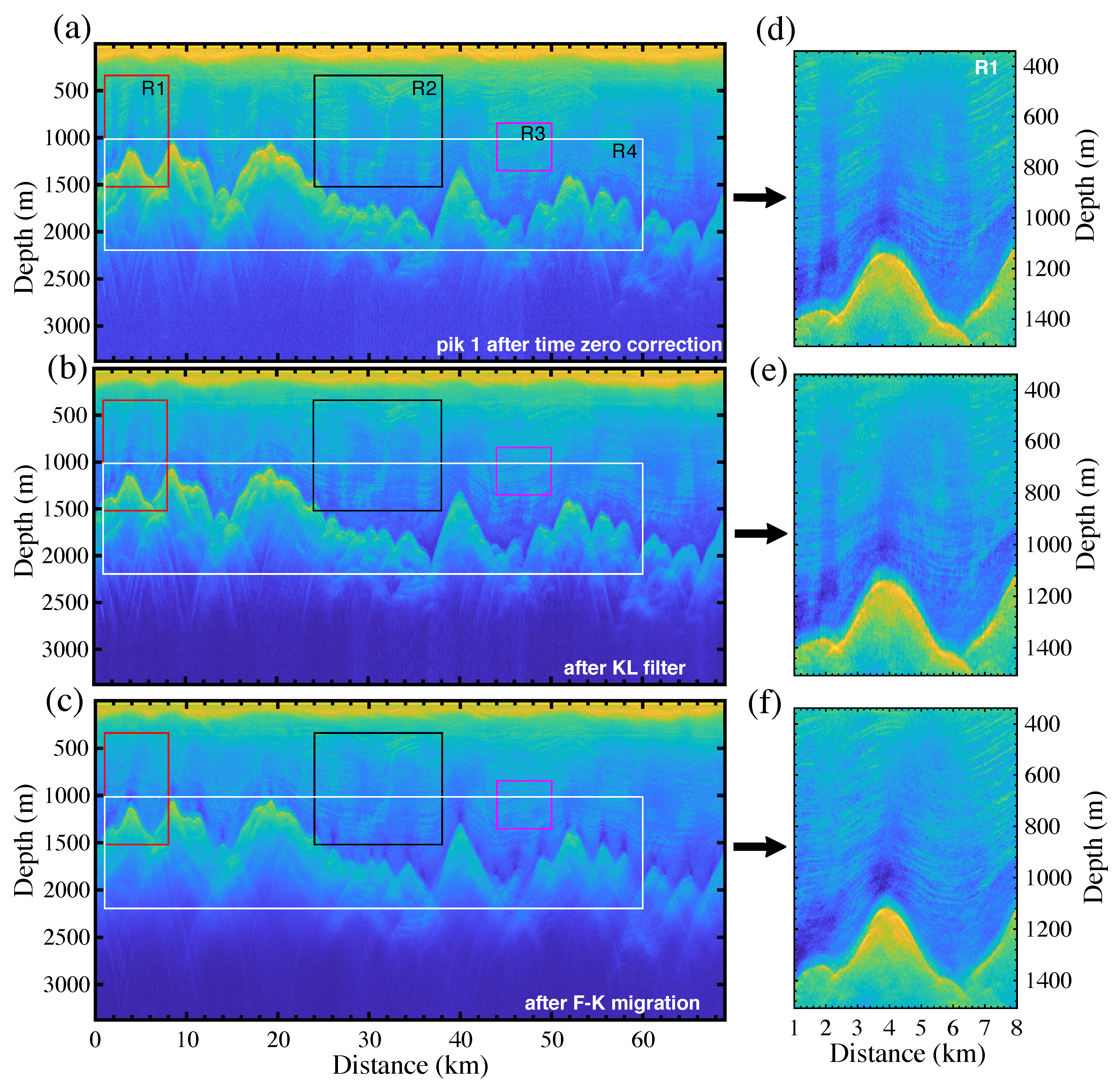
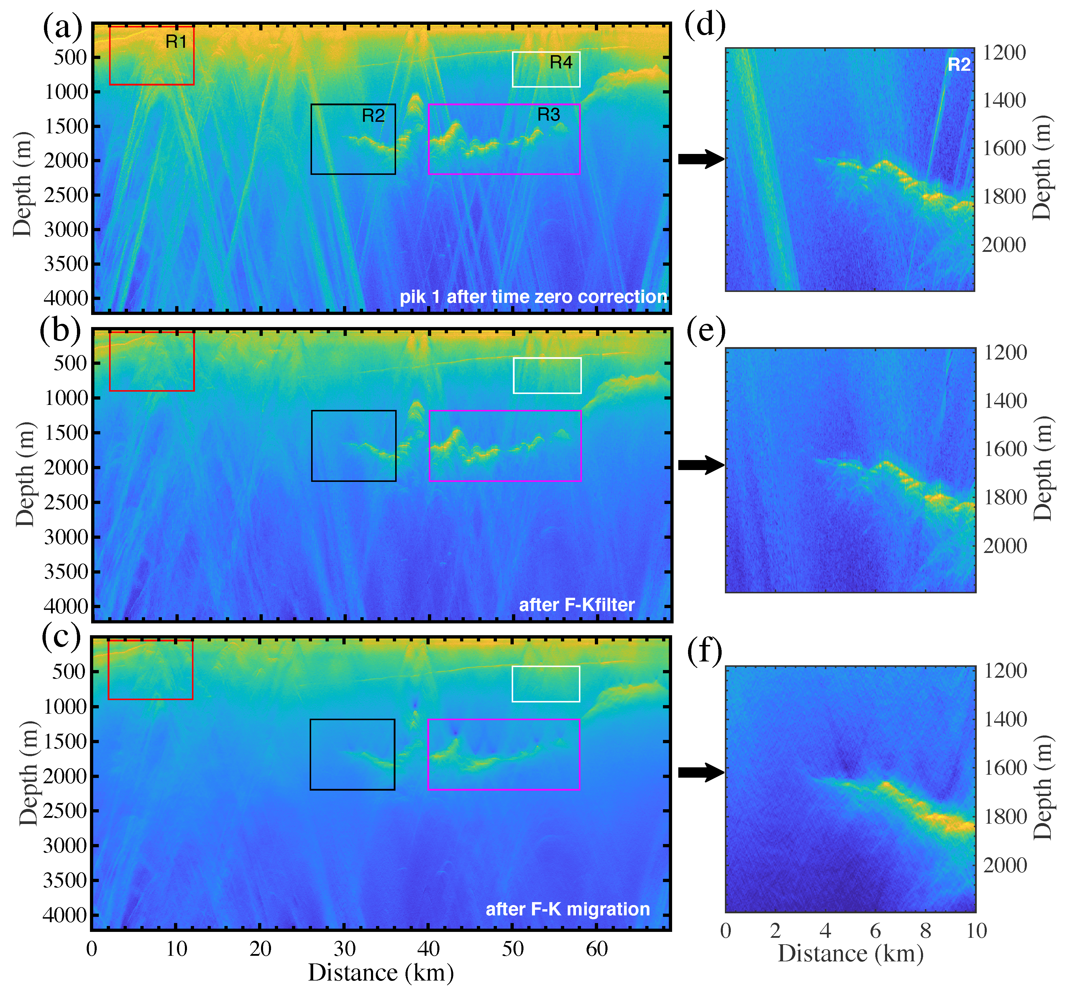
2.2. Results of the Filtering Methods

Figure 2 shows the processing results of Line 1 located inland of the East Antarctic ice sheet after two-dimensional interpolation, removing air, KL filtering, and F–K migration. From the enlarged profiles in the R1 region, the KL filter eliminated the speckle noise. Subsequently, F–K migration further improved the data SNR and not only focused the hyperbolic signal of the ice–rock interface, but also improved the visibility of the internal layers disturbed by aliasing. Figure 3 shows the results of Line 2 across the Amery ice sheet after two-dimensional interpolation, removal of the air layer signal, F–K filtering, and F–K migration processing. The bedrock can be seen at both ends of the transect. Inclined fringes formed by very strong diffracted wave interference cannot be eliminated only by F–K migration, but can be eliminated by setting an appropriate filter window in the F–K domain. As shown in Figure 3b, the inclined fringes were obviously weakened after filtering, and the bedrock was effectively highlighted. The F–K migration in Figure 3c also eliminated some weak hyperbolic inclined fringe interference remaining in Figure 3b. After the above processing flow, the resolution of the profile significantly improved.

Here, three quantitative indexes were used to evaluate the quality of image processing: the equivalent number of looks (ENL), edge protect index (EPI), and peak signal-to-noise ratio (PNSR). The ENL is used to measure the speckle noise suppression effect of the image processing methods. A larger value of the ENL means that the coherent speckle noise suppression effect is better in the image. The ENL is the ratio of the square of the mean value ($E\left[P\right]$) to the variance ($VAR\left[P\right]$) of pixels (P) in a certain area of the image [58,59]. The EPI refers to the ratio of the integral of the gradient difference between the adjacent pixels of the denoised image and the original image, which measures the ability to retain image details. If the value of EPI is closer to one, the edge retention ability of the algorithm is much stronger. The PSNR is an evaluation index of the similarity between the original image and the denoised image. A lower PSNR value implies a better denoising effect, especially when the SNR in the raw image is low. The specific operation formulas of the ENL, EPI, and PSNR are shown in Equations (1)–(3), respectively, as follows:

$$\begin{array}{cc}\mathrm{ENL}=\frac{{\left(E\left[P\right]\right)}^2}{VAR\left[P\right]}& =\frac{{\left[\frac{1}{(2M+1)(2Q+1)}{\sum }_{k=-M}^M{\sum }_{l=-Q}^{Q}D\left(P_i+k,P_j+l\right)\right]}^2}{(2M+1)(2Q+1){\sum }_{j=1}^n{\sum }_{i=1}^m\left\{D\left(P_i+k,P_j+l\right)-E\left[P\right]\right\}}(i=1,2,...,m;j=1,2,,n)\end{array}$$

(1)

$$\mathrm{EPI}=\frac{{\sum }_{j=1}^n{\sum }_{i=1}^m\left|I\left(P_{i+1},P_{j+1}\right)-I\left(P_i,P_j\right)\right|}{{\sum }_{j=1}^n{\sum }_{i=1}^m\left|D\left(P_{i+1},P_{j+1}\right)-D\left(P_i,P_j\right)\right|}$$

(2)

$$\mathrm{PSNR}=10{log}_{10}\left(\frac{{\mathrm{MAX}}_I^2}{\mathrm{MSE}}\right)=10{log}_{10}\left(\frac{{\mathrm{MAX}}_I^2}{\frac{1}{mn}{\sum }_{i=1}^m{\sum }_{j=1}^n\left|\right|I\left(P_i,P_j\right)-D\left(P_i,P_j\right){\left|\right|}^2}\right)$$

(3)

where I and D represent the original image and the denoised image with a size of $m\times n$, respectively; P is the intensity of the pixels; E and VAR are the mean and variance of P; $(P_i,P_j)$ is the position of the pixel in the selected area; M and Q are the window functions used in the calculation, usually both assigned values of two; ${\mathrm{MAX}}_I$ is the maximum value of the image point color; MSE is the mean-squared deviation of the image.

Table 1. Comparisons of quantitative indexes calculated after filtering in the rectangular regions of Line 1 (TSH data; Figure 2).

Rectangle	ENL		EPI		PSNR (dB)
	KL Filter	F–K Migration	KL Filter	F–K Migration	KL Filter	F–K Migration
R1 (r)	308.0	462.7	0.64	0.81	29.2	22.0
R2 (k)	307.8	347.6	0.66	0.75	25.3	20.7
R3 (m)	277.4	269.9	0.66	0.83	22.4	14.5
R4 (w)	105.5	139.6	0.66	0.64	27.4	22.5

and

Table 2. Comparisons of quantitative indexes calculated after filtering in rectangular regions of Line 2 (AMY data; Figure 3).

Rectangle	ENL		EPI		PSNR(dB)
	F–K Filter	F–K Migration	F–K Filter	F–K Migration	F–K filter	F–K Migration
R1 (r)	13.3	79.0	0.87	0.75	23.0	15.9
R2 (k)	7.9	162.0	0.83	0.60	21.1	17.6
R3 (m)	47.3	102.8	0.88	0.43	26.8	20.1
R4 (w)	73.0	95.0	0.99	0.89	23.9	18.9

are the results of the quantitative evaluation indexes of the four rectangular regions selected in the profiles of Line 1 and Line 2, respectively. It is worth noting that the quantitative calculation here was based on the original pik1 data with a low SNR ratio. Therefore, the smaller value of PSNR means a stronger noise suppression ability. As shown in Table 1, F–K migration can further suppress the speckle noise (larger ENL), can maintain the edge details better (larger EPI), and can improve the PSNR by 4.6∼7.9 dB after KL filtering. As shown in Table 2, after FK filtering, F–K migration also further suppressed the speckle noise (larger ENL) and improved the PSNR by 3.5∼7.1 dB, but had a worse edge retention ability (lower EPI). As a large number of strongly inclined fringe interference contained in the pik1 data of Line 2 cover the effective signal, a low EPI value indicates that the fringe interference removal effect is better. In addition, the value of the ENL after F–K migration was lower in the R3 region of Line 2, which may be related to the clear and continuous internal layering and good quality of the pik1 data.

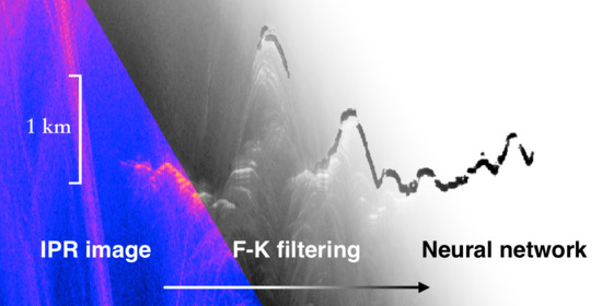
3. Machine Learning Methods

Recently, machine learning methods, especially the sparse dictionary and neural networks, have been widely applied as effective tools in geoscience in place of the experientially manual operation with high efficiency and accuracy [41]. The well-developed machine learning methods make it possible to discriminate the complicated feature between the noise and layers. Visually, the noise and interference in ice radar images, which impede radiostratigraphy research, can be concluded as three main types: (1) Gaussian-like random noise introduced by the instruments and subglacial scatters; (2) vertical shallow fringe interference, which presents the difference between traces; (3) hyperbolic curve-like stripes diffracted from the intense reflection of bedrock interfaces. According to the different characteristics of the noise and methods, appropriate machine-learning-based methods can be applied in noise removal. Here, we demonstrate two approaches to reducing the specified noise and a neural network to resist most of the noise and interference by extracting specific features.

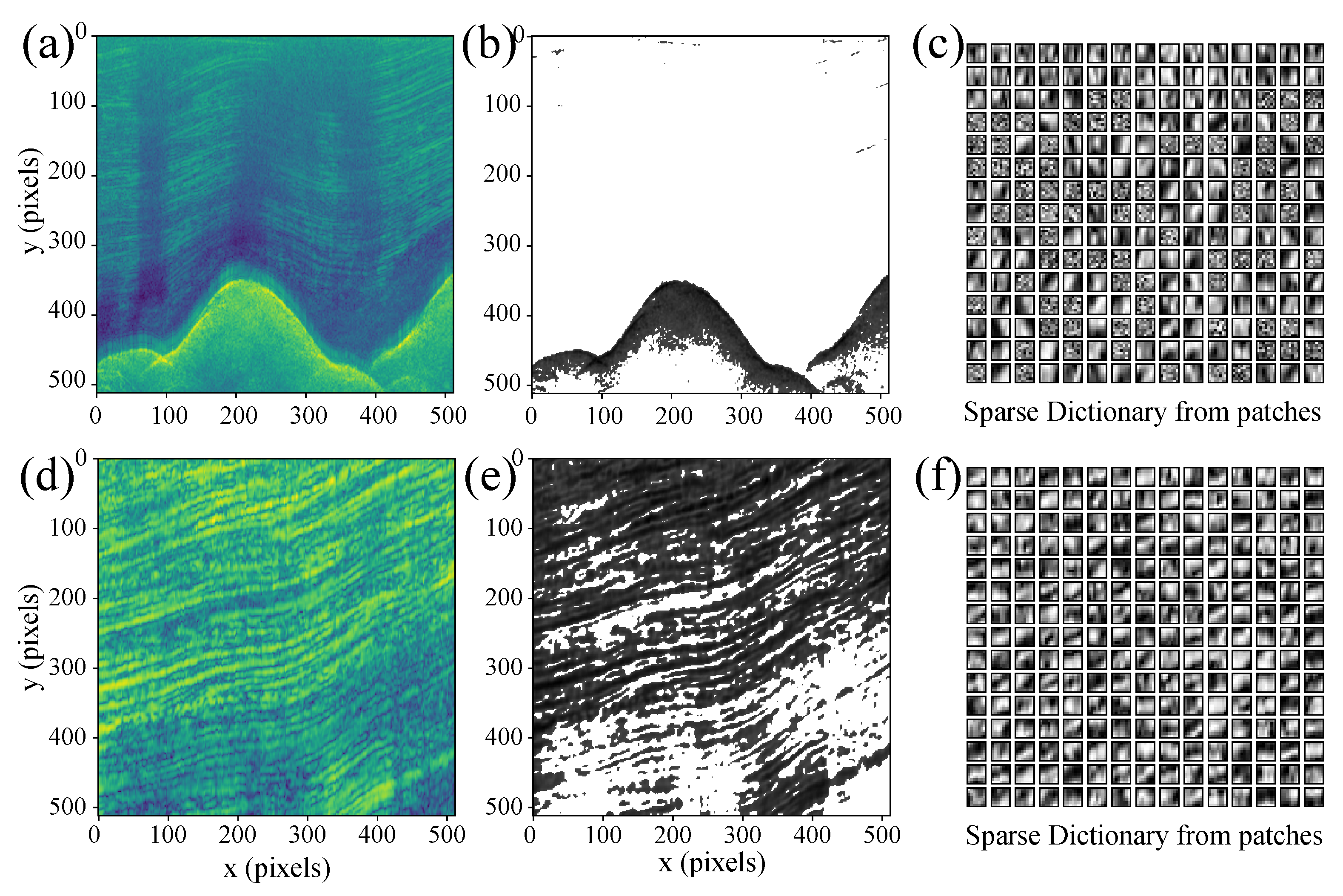
3.1. K-SVD Algorithm

Due to the uncertainty of the noise form and distributions, it is difficult to configure and reconstruct the observational noise in radar images, which also obstructs the application of supervised machine learning methods in noise reductions. Without prior indications as labeling, the unsupervised methods are first applied to exclude noise in the image processing. The K-SVD algorithm [60] has been validated as an effective method to exclude Gaussian noise [61]. As a dictionary-learning-based method, the K-SVD algorithm sparsely represents the patches from the input image as a linear combination of atoms from the redundant dictionary. The K-SVD algorithm uses orthonormal matching pursuit (OMP) [62] to solve:

$$\widehat{a}=\arg \underset{\alpha }{min}{\left|\right|\alpha \left|\right|}_0\mathrm{subject}\mathrm{to}D\alpha \approx x$$

(4)

where $\widehat{a}$ is the sparse representation of x and ${\left|\right|\alpha \left|\right|}_0$ is the count of nonzero entries in $\alpha$. The final denoised image $\widehat{x}$ is obtained by:

$$\widehat{x}=D\widehat{\alpha }$$

(5)

The K-SVD algorithm is widely used in image processing, but limited by the constant shape of image patches. Based on the concept of unsupervised learning, K-SVD learns and decodes the layer feature from patches to the sparse dictionary, in which the random noise is counteracted because of the non-sparse feature. The feature of the boundary between bedrock and ice, which is relatively distinct in observations, is accurately extracted by the water level in amplitude after K-SVD denoising (Figure 4b,e). However, K-SVD suggests low performance in the feature identification of an internal layer, which is fused with noise and visually ambiguous (Figure 4e). The dictionaries learned from patches in raw radar images are shown in Figure 4c,f. As the sizes of the patches are constant, the size of the view fields of K-SVD is stationary, similar to the dictionary. The noise removal of K-SVD was evaluated by the PSNR (Equation (3)), as shown in

Table 3. Comparisons of the PSNRs of K-SVD and the DnCNN in two radar image slices from Line 1 and the quantitative results of the DnCNN and U-Net on the $10\%$ reserved from the training dataset.

Data	PSNR (dB)		Precision		Recall		F1-Score
	K-SVD	DnCNN	U-Net	DnCNN	U-Net	DnCNN	U-Net	DnCNN
Line 1 (R1)	16.401	35.757	-	-	-	-	-	-
Line 1 (R3)	7.548	32.420	-	-	-	-	-	-
Test Dataset	-	-	0.501	0.299	0.293	0.286	0.375	0.292

.

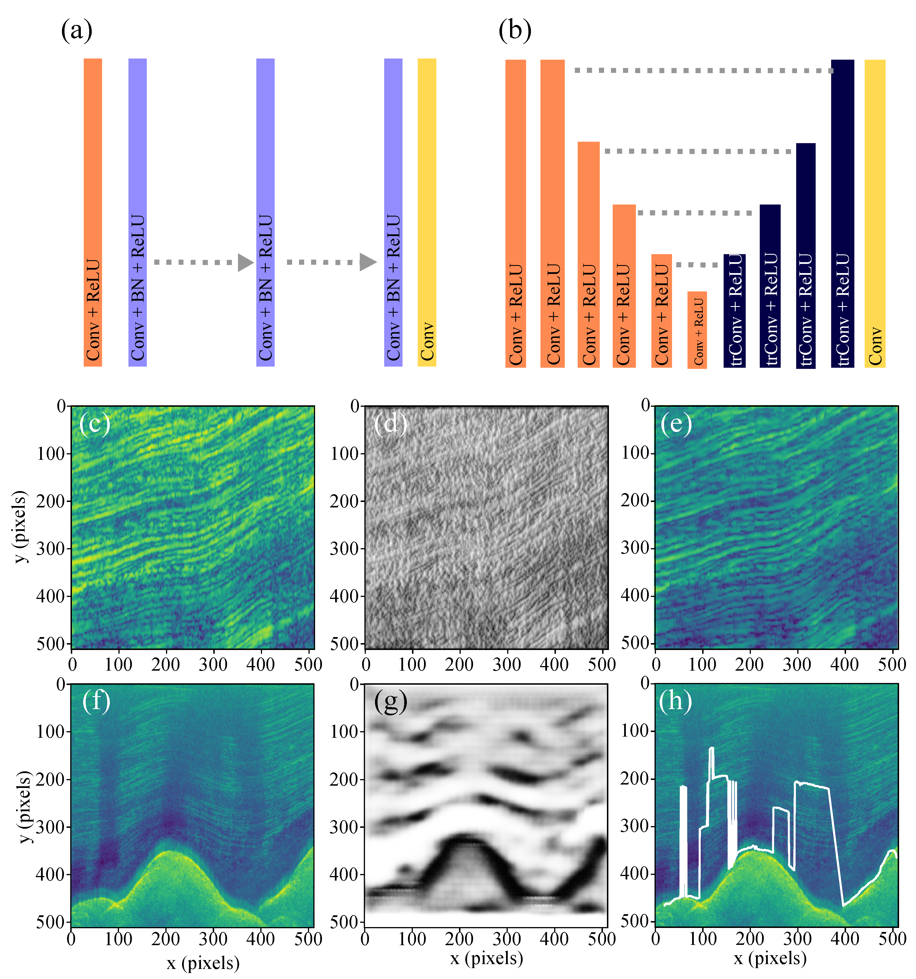
3.2. Artificial Neural Networks

In recent decades, the convolutional neural network (CNN) [63] has commonly been applied in visual imagery processing, including regression, classification, and segmentation. Based on the concept of deep residual learning [64], the DnCNN [65] learns from the residual distribution of the noise, which can be reduced by subtraction from the raw image. As a denoiser, the DnCNN is not only able to reduce Gaussian denoising with unknown noise levels, but is also able to further be extended in the removal of other types of noise, such as the block-like interference in a jpeg image. The architecture of the DnCNN is shown in Figure 5a, in which the color of the bars represents the difference of the layers used in the network, and the abbreviations of the layer types are also appended. The length of the bars indicates the relative width of the data flow from the convolutional layer (abbr. Conv), transpose convolutional layer (abbr. trConv), and batch normalization layer (abbr. BN). The activation used in the network is the rectified linear unit (ReLU). We demonstrate the application of the DnCNN in radar images (Figure 5c–e) after 100 epochs trained on 500 synthetic radar images, which contained Gaussian noise and were generated by the method introduced in Dong and others [45]. Similar to the results of the K-SVD method, the Gaussian-like noise was reduced, but the localized features of interference, such as stripes and fringes, still existed in the denoised result. The noise removal of the DnCNN was also evaluated by the PSNR (Equation (3)), as shown in Table 3. The difference between the DnCNN and K-SVD revealed the higher performance of the DnCNN in noise removal. Moreover, the higher PSNR than that in the result after conventional filtering methods in the same area (R1 and R3 in Line 1; Table 1) statistically suggests a better effect on the reduction in noise by the DnCNN.

The denoising methods above showed the capacities of the Gaussian-like random noise removal. However, for the noise types (2) and (3), the precise distribution of interference is hard to evaluate, and hence cannot be reduced. Another approach to feature tracing from radar images is to directly extract the features of layers, including the internal layers and bedrock interfaces. Based on the skip connection in the encoder–decoder structure, the CNN has obtained high benchmarks in the image segmentation task [66]. The architecture of U-Net is shown in Figure 5b. The human-indicated label of the bedrock interface and internal layers from observational radar images provides sufficient materials for the training of neural networks [38,42,43]. Figure 5f,g shows the prediction of U-Net in the bedrock interface. The network was trained on 87 slices from CHINARE with manually extracted labels after 30 epochs. The extraction result after grid searching in the predicted matrix is shown in Figure 5h as the white curve, in which the obstruction of the mistaken prediction of the layer features is also demonstrated. We used the fresh data to quantitatively analyze the DnCNN and U-Net in one-hundred and eight image slices, respectively, as shown in the last line of Table 3. The result showed relatively low accuracy for U-Net, which may be caused by the lack in the number and quality of manual labels applied in training.

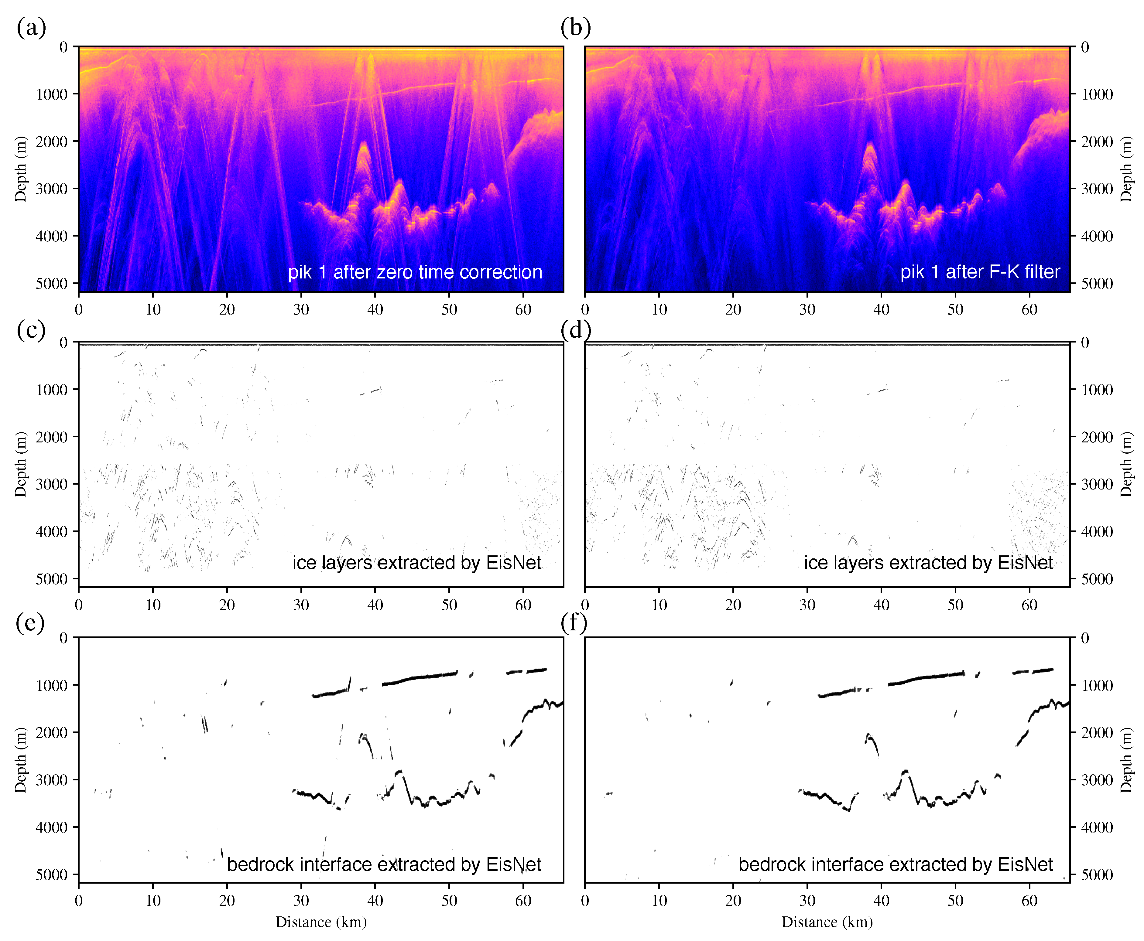
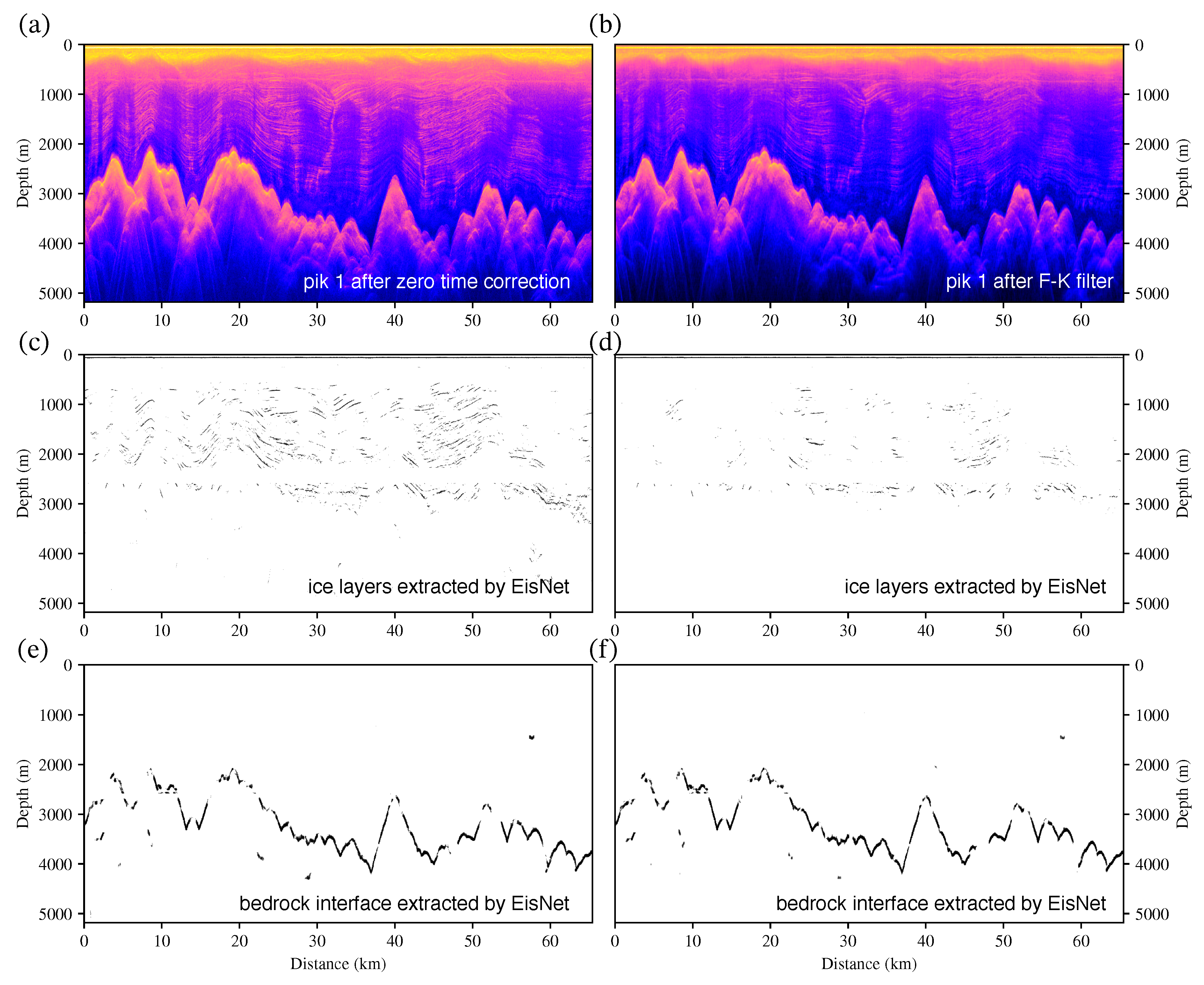
4. Fusion Applications of the Methods

In general, the F–K and KL filtering methods reveal reliable performance in single-feature textures, as mentioned above. The machine learning methods yield effective results in Gaussian noise removal and layer feature extraction as well. The EisNet was recently proposed to extract the internal layers and bedrock interface simultaneously with accuracy [45]. To unify the advantages of the methods and to optimize the extraction of the layer features, we further assembled the conventional methods in the preprocessing with the machine-learning-based method as the following extractor. Here, we used the same radar images in Figure 2 and Figure 3 to demonstrate the combined applications of F–K/KL filtering and the trained EisNet (as shown in Figure 6 and Figure 7).

The results in Figure 6 suggest that the extraction of the bedrock interface benefits from the preprocessing of F–K filtering, which reduces the hyperbolic signal before neural network extraction. The features of the internal layers are relatively ambiguous in both raw and filtered radar images; thus, the extracted internal layers are meaningless, as in Figure 6c,d. In contrast, the results shown in Figure 7e,f indicate a trivial difference in extractions before and after KL filtering, which implies that the machine-learning-based method presents a high capacity in feature identification. The comparison in Figure 7c,d shows a large decrease in internal layer extractions after KL filtering, which further indicates that the filtering is not as necessary as in the example in Figure 6. By considering the multiple methods and various types of noise, we suggest using the combined method for the condition in which the hyperbolic signal significantly affects the feature presentations in radar images, as in Figure 6.

On the other hand, the neural network method converts the input to binary results, which reduces nearly all features except for the features of internal layers and the bedrock interface. Therefore, ideally, the comparison of neural network extractions would be considered to evaluate the lost features of internal layers and the bedrock in the conventional filtering method. As shown in Figure 6c–f and Figure 7c–f, the filtering methods removed the specific features (e.g., the hyperbolic signal) in the global radar images, which optimized the presentations of the bedrock’s feature. However, the internal layers’ feature may fail in the localized area, which is dependent on the method and parameters used in the filtering. Moreover, we quantitatively evaluated the influence of filtering by calculating the PSNRs (Equation (3)) between the yielded feature distribution (binary results) and input radar image from two lines. The PSNRs show coinciding result with the extracted internal layer in Figure 6 and Figure 7. The first row in

Table 4. Comparisons of the PSNRs before and after filtering in two lines. The PSNRs are calculated by the MSE between the neural-network-extracted feature and input radar image.

Line	PSNR (dB)
	Before Filtering	After Filtering
Line 2 (AMY)	7.769	8.127
Line 1 (TSH)	9.384	7.277

reveals the promotion of the layer feature after F–K filtering. In contrast, the second row in Table 4 indicates the reduction in features after KL filtering. The comparisons of the PSNRs suggest that more noise and interferes were reduced in Line 2 (AMY data) after F–K filtering, whereas the decreasing PSNR in Line 1 (TSH data) reveals that more features from raw radar images, which could be extracted as layers by the EisNet, were reduced after KL filtering.

5. Conclusions

To enhance the feature presentations in IPR data, filtering methods are applied in the removal of feature noise and interference. In recent decades, machine-learning-based methods have improved the efficiency and accuracy of layer extraction from field radar data. We first compared the removal of fringe interference by F–K and KL filtering and second demonstrated the reduction in noise by the machine-learning-based DnCNN and K-SVD methods, as well as the extraction of bedrock interfaces by U-Net. The result suggests that the specific fringe interference can be effectively reduced using the filtering method and that machine-learning-based methods show good performance in layer extraction. Therefore, we proposed a fusion method based on filtering methods and machine learning. This fusion method provides an automatic approach in layer extraction with the advantages of both F–K of KL filtering in interference removal and the neural network in layer feature extraction. This method has potential applications to IPR data from the Antarctic and Greenland ice sheets as a constant strategy to rapidly extract features.

References

1. Hanna, E.; Pattyn, F.; Navarro, F.; Favier, V.; Goelzer, H.; van den Broeke, M.R.; Vizcaino, M.; Whitehouse, P.L.; Ritz, C.; Bulthuis, K.; et al. Mass balance of the ice sheets and glaciers–progress since AR5 and challenges. Earth-Sci. Rev. 2020, 201, 102976. [Google Scholar] [CrossRef]
2. Poloczanska, E.; Mintenbeck, K.; Portner, H.O.; Roberts, D.; Levin, L.A. The IPCC special report on the ocean and cryosphere in a changing climate. In Proceedings of the 2018 Ocean Sciences Meeting, Portland, OR, USA, 11–16 February 2018. [Google Scholar]
3. Mouginot, J.; Rignot, E.; Scheuchl, B. Sustained increase in ice discharge from the Amundsen Sea Embayment, West Antarctica, from 1973 to 2013. Geophys. Res. Lett. 2014, 41, 1576–1584. [Google Scholar] [CrossRef] [Green Version]
4. Shepherd, A.; Ivins, E.; Rignot, E.; Smith, B.; Van Den Broeke, M.; Velicogna, I.; Whitehouse, P.; Briggs, K.; Joughin, I.; Krinner, G.; et al. Mass balance of the Antarctic Ice Sheet from 1992 to 2017. Nature 2018, 558, 219–222. [Google Scholar]
5. Rignot, E.; Mouginot, J.; Scheuchl, B.; Van Den Broeke, M.; Van Wessem, M.J.; Morlighem, M. Four decades of Antarctic Ice Sheet mass balance from 1979–2017. Proc. Natl. Acad. Sci. USA 2019, 116, 1095–1103. [Google Scholar] [CrossRef] [PubMed] [Green Version]
6. Winter, K.; Woodward, J.; Ross, N.; Dunning, S.A.; Hein, A.S.; Westoby, M.J.; Culberg, R.; Marrero, S.M.; Schroeder, D.M.; Sugden, D.E.; et al. Radar-detected englacial debris in the West Antarctic Ice Sheet. Geophys. Res. Lett. 2019, 46, 10454–10462. [Google Scholar]
7. Bodart, J.A.; Bingham, R.G.; Ashmore, D.W.; Karlsson, N.B.; Hein, A.; Vaughan, D.G. Age-depth stratigraphy of Pine Island Glacier inferred from airborne radar and ice-core chronology. J. Geophys. Res. Earth Surf. 2021, 126, e2020JF005927. [Google Scholar] [CrossRef]
8. Cavitte, M.G.; Young, D.A.; Mulvaney, R.; Ritz, C.; Greenbaum, J.S.; Ng, G.; Kempf, S.D.; Quartini, E.; Muldoon, G.R.; Paden, J.; et al. A detailed radiostratigraphic data set for the central East Antarctic Plateau spanning from the Holocene to the mid-Pleistocene. Earth Syst. Sci. Data 2021, 13, 4759–4777. [Google Scholar] [CrossRef]
9. MacGREGOR, J.A.; Anandakrishnan, S.; Catania, G.A.; Winebrenner, D.P. The grounding zone of the Ross Ice Shelf, West Antarctica, from ice-penetrating radar. J. Glaciol. 2011, 57, 917–928. [Google Scholar] [CrossRef] [Green Version]
10. Reese, R.; Gudmundsson, G.H.; Levermann, A.; Winkelmann, R. The far reach of ice-shelf thinning in Antarctica. Nat. Clim. Chang. 2018, 8, 53–57. [Google Scholar] [CrossRef]
11. Robin, G.d.Q. Radio-echo sounding: Glaciological interpretations and applications. J. Glaciol. 1975, 15, 49–64. [Google Scholar] [CrossRef] [Green Version]
12. Fretwell, P.; Pritchard, H.D.; Vaughan, D.G.; Bamber, J.L.; Barrand, N.E.; Bell, R.; Bianchi, C.; Bingham, R.; Blankenship, D.D.; Casassa, G.; et al. Bedmap2: Improved ice bed, surface and thickness datasets for Antarctica. Cryosphere 2013, 7, 375–393. [Google Scholar] [CrossRef] [Green Version]
13. Schroeder, D.M.; Bingham, R.G.; Blankenship, D.D.; Christianson, K.; Eisen, O.; Flowers, G.E.; Karlsson, N.B.; Koutnik, M.R.; Paden, J.D.; Siegert, M.J. Five decades of radioglaciology. Ann. Glaciol. 2020, 61, 1–13. [Google Scholar] [CrossRef] [Green Version]
14. Matsuoka, K. Pitfalls in radar diagnosis of ice-sheet bed conditions: Lessons from englacial attenuation models. Geophys. Res. Lett. 2011, 38. [Google Scholar] [CrossRef]
15. Tang, X.; Sun, B.; Wang, T. Radar isochronic layer dating for a deep ice core at Kunlun Station, Antarctica. Sci. China Earth Sci. 2020, 63, 303–308. [Google Scholar] [CrossRef]
16. Bons, P.D.; Jansen, D.; Mundel, F.; Bauer, C.C.; Binder, T.; Eisen, O.; Jessell, M.W.; Llorens, M.G.; Steinbach, F.; Steinhage, D.; et al. Converging flow and anisotropy cause large-scale folding in Greenland’s ice sheet. Nat. Commun. 2016, 7, 11427. [Google Scholar] [CrossRef] [PubMed] [Green Version]
17. Cooper, M.; Jordan, T.; Siegert, M.; Bamber, J. Surface expression of basal and englacial features, properties, and processes of the Greenland ice sheet. Geophys. Res. Lett. 2019, 46, 783–793. [Google Scholar] [CrossRef] [Green Version]
18. Bingham, R.G.; Rippin, D.M.; Karlsson, N.B.; Corr, H.F.; Ferraccioli, F.; Jordan, T.A.; Le Brocq, A.M.; Rose, K.C.; Ross, N.; Siegert, M.J. Ice-flow structure and ice dynamic changes in the Weddell Sea sector of West Antarctica from radar-imaged internal layering. J. Geophys. Res. Earth Surf. 2015, 120, 655–670. [Google Scholar] [CrossRef] [Green Version]
19. Elsworth, C.W.; Schroeder, D.M.; Siegfried, M.R. Interpreting englacial layer deformation in the presence of complex ice flow history with synthetic radargrams. Ann. Glaciol. 2020, 61, 206–213. [Google Scholar] [CrossRef] [Green Version]
20. Jordan, T.M.; Cooper, M.A.; Schroeder, D.M.; Williams, C.N.; Paden, J.D.; Siegert, M.J.; Bamber, J.L. Self-affine subglacial roughness: Consequences for radar scattering and basal water discrimination in northern Greenland. Cryosphere 2017, 11, 1247–1264. [Google Scholar] [CrossRef] [Green Version]
21. Luo, K.; Liu, S.; Guo, J.; Wang, T.; Li, L.; Cui, X.; Sun, B.; Tang, X. Radar-Derived Internal Structure and Basal Roughness Characterization along a Traverse from Zhongshan Station to Dome A, East Antarctica. Remote Sens. 2020, 12, 1079. [Google Scholar] [CrossRef] [Green Version]
22. Jordan, T.; Martin, C.; Ferraccioli, F.; Matsuoka, K.; Corr, H.; Forsberg, R.; Olesen, A.; Siegert, M. Anomalously high geothermal flux near the South Pole. Sci. Rep. 2018, 8, 16785. [Google Scholar] [CrossRef] [Green Version]
23. Wolovick, M.; Moore, J.; Zhao, L. Joint Inversion for Surface Accumulation Rate and Geothermal Heat Flow from Ice-Penetrating Radar Observations at Dome A, East Antarctica. Part I: Model Description, Data Constraints, and Inversion Results. J. Geophys. Res. Earth Surf. 2021, 126, e2020JF005937. [Google Scholar] [CrossRef]
24. Young, D.; Schroeder, D.; Blankenship, D.; Kempf, S.D.; Quartini, E. The distribution of basal water between Antarctic subglacial lakes from radar sounding. Philos. Trans. R. Soc. Math. Phys. Eng. Sci. 2016, 374, 20140297. [Google Scholar] [CrossRef]
25. Jordan, T.M.; Williams, C.N.; Schroeder, D.M.; Martos, Y.M.; Cooper, M.A.; Siegert, M.J.; Paden, J.D.; Huybrechts, P.; Bamber, J.L. A constraint upon the basal water distribution and thermal state of the Greenland Ice Sheet from radar bed echoes. Cryosphere 2018, 12, 2831–2854. [Google Scholar] [CrossRef] [Green Version]
26. Wang, B.; Sun, B.; Wang, J.; Greenbaum, J.; Guo, J.; Lindzey, L.; Cui, X.; Young, D.A.; Blankenship, D.D.; Siegert, M.J. Removal of ‘strip noise’ in radio-echo sounding data using combined wavelet and 2-D DFT filtering. Ann. Glaciol. 2020, 61, 124–134. [Google Scholar] [CrossRef] [Green Version]
27. Heister, A.; Scheiber, R. Coherent large beamwidth processing of radio-echo sounding data. Cryosphere 2018, 12, 2969–2979. [Google Scholar] [CrossRef]
28. Lilien, D.A.; Hills, B.H.; Driscol, J.; Jacobel, R.; Christianson, K. ImpDAR: An open-source impulse radar processor. Ann. Glaciol. 2020, 61, 114–123. [Google Scholar] [CrossRef]
29. Partyka, G.; Gridley, J.; Lopez, J. Interpretational applications of spectral decomposition in reservoir characterization. Lead. Edge 1999, 18, 353–360. [Google Scholar] [CrossRef] [Green Version]
30. Wu, Z.; Huang, N.E. A study of the characteristics of white noise using the empirical mode decomposition method. Proc. R. Soc. London. Ser. A Math. Phys. Eng. Sci. 2004, 460, 1597–1611. [Google Scholar] [CrossRef]
31. Huang, N.E.; Shen, Z.; Long, S.R.; Wu, M.C.; Shih, H.H.; Zheng, Q.; Yen, N.C.; Tung, C.C.; Liu, H.H. The empirical mode decomposition and the Hilbert spectrum for nonlinear and non-stationary time series analysis. Proc. R. Soc. Lond. Ser. A Math. Phys. Eng. Sci. 1998, 454, 903–995. [Google Scholar] [CrossRef]
32. Dragomiretskiy, K.; Zosso, D. Variational mode decomposition. IEEE Trans. Signal Process. 2013, 62, 531–544. [Google Scholar] [CrossRef]
33. Cheng, S.; Liu, S.; Guo, J.; Luo, K.; Zhang, L.; Tang, X. Data processing and interpretation of Antarctic ice-penetrating radar based on variational mode decomposition. Remote Sens. 2019, 11, 1253. [Google Scholar] [CrossRef] [Green Version]
34. Zhu, Y.; Zhang, S.; Zhao, H.; Chen, S. Target Identification with Improved 2D-VMD for Carrier-Free UWB Radar. Sensors 2021, 21, 2465. [Google Scholar] [CrossRef]
35. Xiong, S.; Muller, J.P.; Carretero, R.C. A new method for automatically tracing englacial layers from MCoRDS data in NW Greenland. Remote Sens. 2018, 10, 43. [Google Scholar] [CrossRef] [Green Version]
36. Berger, V.; Xu, M.; Chu, S.; Crandall, D.; Paden, J.; Fox, G.C. Automated tracking of 2D and 3D ice radar imagery using VITERBI and TRW-S. In Proceedings of the IGARSS 2018—2018 IEEE International Geoscience and Remote Sensing Symposium, Honolulu, HI, USA, 25–30 July 2010; IEEE: Piscataway, NJ, USA, 2018; pp. 4162–4165. [Google Scholar]
37. Donini, E.; Thakur, S.; Bovolo, F.; Bruzzone, L. An automatic approach to map refreezing ice in radar sounder data. In Image and Signal Processing for Remote Sensing XXV; International Society for Optics and Photonics: Strasbourg, France, 2019; Volume 11155, p. 111551B. [Google Scholar]
38. Rahnemoonfar, M.; Yari, M.; Paden, J.; Koenig, L.; Ibikunle, O. Deep multi-scale learning for automatic tracking of internal layers of ice in radar data. J. Glaciol. 2021, 67, 39–48. [Google Scholar] [CrossRef]
39. Castelletti, D.; Schroeder, D.M.; Hensley, S.; Grima, C.; Ng, G.; Young, D.; Gim, Y.; Bruzzone, L.; Moussessian, A.; Blankenship, D.D. An interferometric approach to cross-track clutter detection in two-channel VHF radar sounders. IEEE Trans. Geosci. Remote Sens. 2017, 55, 6128–6140. [Google Scholar] [CrossRef]
40. Delf, R.; Schroeder, D.M.; Curtis, A.; Giannopoulos, A.; Bingham, R.G. A comparison of automated approaches to extracting englacial-layer geometry from radar data across ice sheets. Ann. Glaciol. 2020, 61, 234–241. [Google Scholar] [CrossRef]
41. Bergen, K.J.; Johnson, P.A.; Maarten, V.; Beroza, G.C. Machine learning for data-driven discovery in solid Earth geoscience. Science 2019, 363. [Google Scholar] [CrossRef]
42. Rahnemoonfar, M.; Fox, G.C.; Yari, M.; Paden, J. Automatic ice surface and bottom boundaries estimation in radar imagery based on level-set approach. IEEE Trans. Geosci. Remote Sens. 2017, 55, 5115–5122. [Google Scholar] [CrossRef]
43. Ibikunle, O.; Paden, J.; Rahnemoonfar, M.; Crandall, D.; Yari, M. Snow Radar Layer Tracking Using Iterative Neural Network Approach. In Proceedings of the IGARSS 2020—2020 IEEE International Geoscience and Remote Sensing Symposium, Waikoloa, HI, USA, 26 September–2 October 2020; pp. 2960–2963. [Google Scholar] [CrossRef]
44. Khami, N.; Imtiaz, O.; Abidi, A.; Aedavelli, A.; Goff, A.; Pisel, J.R.; Pyrcz, M.J. Automatic Feature Highlighting in Noisy RES Data With CycleGAN. arXiv 2021, arXiv:2108.11283. [Google Scholar]
45. Dong, S.; Tang, X.; Guo, J.; Fu, L.; Chen, X.; Sun, B. EisNet: Extracting Bedrock and Internal Layers from Radiostratigraphy of Ice Sheets with Machine Learning. IEEE Trans. Geosci. Remote Sens. 2021, 1. [Google Scholar] [CrossRef]
46. Young, D.A.; Wright, A.P.; Roberts, J.L.; Warner, R.C.; Young, N.W.; Greenbaum, J.S.; Schroeder, D.M.; Holt, J.W.; Sugden, D.E.; Blankenship, D.D.; et al. A dynamic early East Antarctic Ice Sheet suggested by ice-covered fjord landscapes. Nature 2011, 474, 72–75. [Google Scholar] [CrossRef]
47. Greenbaum, J.; Blankenship, D.; Young, D.; Richter, T.; Roberts, J.; Aitken, A.; Legresy, B.; Schroeder, D.; Warner, R.; Van Ommen, T.; et al. Ocean access to a cavity beneath Totten Glacier in East Antarctica. Nat. Geosci. 2015, 8, 294–298. [Google Scholar] [CrossRef]
48. Cavitte, M.G.; Blankenship, D.D.; Young, D.A.; Schroeder, D.M.; Parrenin, F.; Lemeur, E.; Macgregor, J.A.; Siegert, M.J. Deep radiostratigraphy of the East Antarctic plateau: Connecting the Dome C and Vostok ice core sites. J. Glaciol. 2016, 62, 323–334. [Google Scholar] [CrossRef] [Green Version]
49. Lindzey, L.E.; Beem, L.H.; Young, D.A.; Quartini, E.; Blankenship, D.D.; Lee, C.K.; Lee, W.S.; Lee, J.I.; Lee, J. Aerogeophysical characterization of an active subglacial lake system in the David Glacier catchment, Antarctica. Cryosphere 2020, 14, 2217–2233. [Google Scholar] [CrossRef]
50. Peters, M.E.; Blankenship, D.D.; Carter, S.P.; Kempf, S.D.; Young, D.A.; Holt, J.W. Along-track focusing of airborne radar sounding data from West Antarctica for improving basal reflection analysis and layer detection. IEEE Trans. Geosci. Remote Sens. 2007, 45, 2725–2736. [Google Scholar] [CrossRef]
51. Cui, X.; Jeofry, H.; Greenbaum, J.S.; Guo, J.; Li, L.; Lindzey, L.E.; Habbal, F.A.; Wei, W.; Young, D.A.; Ross, N.; et al. Bed topography of Princess Elizabeth Land in East Antarctica. Earth Syst. Sci. Data 2020, 12, 2765–2774. [Google Scholar] [CrossRef]
52. Tzanis, A. matGPR Release 2: A freeware MATLAB® package for the analysis & interpretation of common and single offset GPR data. FastTimes 2010, 15, 17–43. [Google Scholar]
53. Karhunen, K. Zur spektraltheorie stochastischer prozesse. Ann. Acad. Sci. Fennicae AI 1946, 34, 215–220. [Google Scholar]
54. Loeve, M. Probability theory. Foundations. Random sequences. Van Nostrand 1955, 33, 5–16. [Google Scholar]
55. Kawalec, A.; Owczarek, R.; Dudczyk, J. Karhunen-Loeve transformation in radar signal features processing. In Proceedings of the 2006 International Conference on Microwaves, Radar & Wireless Communications, Krakow, Poland, 22-24 May 2006; IEEE: Piscataway, NJ, USA, 2006; pp. 1168–1171. [Google Scholar]
56. Haizhong, Y.; Xiaojian, Y. Derivative seismic processing method for GPR data. In IGARSS’97, Proceedings of the 1997 IEEE International Geoscience and Remote Sensing Symposium Proceedings.; Remote Sensing—A Scientific Vision for Sustainable Development, Singapore, 3–8 August 1997; IEEE: Piscataway, NJ, USA, 1997; Volume 1, pp. 145–147. [Google Scholar]
57. Wei, X.; Zhang, Y. Interference removal for autofocusing of GPR data from RC bridge decks. IEEE J. Sel. Top. Appl. Earth Obs. Remote Sens. 2015, 8, 1145–1151. [Google Scholar] [CrossRef]
58. Moreira, A. Improved multilook techniques applied to SAR and SCANSAR imagery. IEEE Trans. Geosci. Remote Sens. 1991, 29, 529–534. [Google Scholar] [CrossRef]
59. Lang, S. Research on the Imaging and Signal Processing of High-Resolution Ice-Sounding Radar. Ph.D. Thesis, University of Chinese Academy of Sciences, Beijing, China, 2015. [Google Scholar]
60. Aharon, M.; Elad, M.; Bruckstein, A. K-SVD: An algorithm for designing overcomplete dictionaries for sparse representation. IEEE Trans. Signal Process. 2006, 54, 4311–4322. [Google Scholar] [CrossRef]
61. Elad, M.; Aharon, M. Image denoising via sparse and redundant representations over learned dictionaries. IEEE Trans. Image Process. 2006, 15, 3736–3745. [Google Scholar] [CrossRef] [PubMed]
62. Pati, Y.C.; Rezaiifar, R.; Krishnaprasad, P.S. Orthogonal matching pursuit: Recursive function approximation with applications to wavelet decomposition. In Proceedings of the 27th Asilomar Conference on Signals, Systems and Computers, Pacific Grove, CA, USA, 1–3 November 1993; IEEE: Piscataway, NJ, USA, 1993; pp. 40–44. [Google Scholar]
63. Krizhevsky, A.; Sutskever, I.; Hinton, G.E. Imagenet classification with deep convolutional neural networks. Adv. Neural Inf. Process. Syst. 2012, 25, 1097–1105. [Google Scholar] [CrossRef]
64. He, K.; Zhang, X.; Ren, S.; Sun, J. Deep residual learning for image recognition. In Proceedings of the IEEE Conference on Computer Vision and Pattern Recognition, Las Vegas, NV, USA, 27–30 June 2016; IEEE: Piscataway, NJ, USA, 2016; pp. 770–778. [Google Scholar]
65. Zhang, K.; Zuo, W.; Chen, Y.; Meng, D.; Zhang, L. Beyond a Gaussian denoiser: Residual learning of deep cnn for image denoising. IEEE Trans. Image Process. 2017, 26, 3142–3155. [Google Scholar] [CrossRef] [PubMed] [Green Version]
66. Ronneberger, O.; Fischer, P.; Brox, T. U-net: Convolutional networks for biomedical image segmentation. In Proceedings of the International Conference on Medical Image Computing and Computer-Assisted Intervention, Munich, Germany, 5–9 October 2015; Springer: Berlin/Heidelberg, Germany, 2015; pp. 234–241. [Google Scholar]
Figure 1. (a) Locations of the two selected airborne IPR data. Line 1 (green line) is part of the line named TSH_TRV01b (abbr. TSH), which was collected during CHINARE 32 (2015/2016), and Line 2 (red line), named AMY_Y335a (abbr. AMY), was collected during CHINARE 34 (2017/2018). The vectors in the green line and red line indicate the directions of the flights. (b) Schematic airborne IPR transect showing the resultant radar waves and a hyperbola geometry for a strong point reflector. Red stars indicate the position of the aircraft.
Remotesensing 14 00399 g001
Figure 2. Radar data and processing results of Line 1 (TSH data). (ac) are the results of time zero correction (two-dimensional interpolation and removal of the air layer signal), KL filtering, and F–K migration in the processing sequence. The rectangular boxes in the profile are the four areas selected for quantitative evaluation index calculation (R1—red; R2—black; R3—magenta; and R4—white). (df) are the corresponding R1 areas in (ac), respectively.
Remotesensing 14 00399 g002
Figure 3. Radar data and processing results of Line 2 (AMY data). (ac) are the results of time zero correction (two-dimensional interpolation and removal of the air layer signal), F–K filtering, and F–K migration in the processing sequence. The rectangular boxes in the profile are the four areas selected for quantitative evaluation index calculation (R1—red; R2—black; R3—magenta; and R4—white). (df) are the corresponding R2 areas in (ac), respectively.
Remotesensing 14 00399 g003
Figure 4. The extracted internal layers from denoised radar images from K-SVD. (a) The raw input of the radar image, which contains features of both the bedrock and internal layer and from R3 slices of Line 1; Figure 2. (b) The extraction of features by applying a 0.5 threshold in the denoised radar image. (c) The sparse dictionary learns from the patches from the input radar image from R1 slices of Line 1; Figure 2. (d) The raw input of the radar image, which contains the features of internal layers only. (e) Extracted feature by a 0.5 threshold in the denoised radar image from K-SVD. (f) The sparse dictionary learns from the patches from the input radar image.
Remotesensing 14 00399 g004
Figure 5. Structures of the DnCNN and U-Net that are applied in denoising and extraction and a demonstration of the denoise and bedrock interface extraction. (a) The network structure of the DnCNN for imagery denoising, in which the dash vectors present the data flow. (b) The network structure of U-Net for feature extraction, in which the gray dashed line presents the skip connections between layers. (c) The input radar image from R3 slices of Line 1 (Figure 2) for validation of DnCNN denoising. (d) The extracted noise from the input radar image. (e) The denoised result of radar image slices. (f) The input radar image from the R1 slices of Line 1 (Figure 2) for U-Net extraction. (g) The distribution of extracted bedrock interface features. (h) Comparison between the input radar image and the extracted bedrock.
Remotesensing 14 00399 g005
Figure 6. Comparison of EisNet extractions before and after F–K filtering from Line 2 (AMY data). (a) The raw input radar image. (b) The input radar image after F–K filtering as a preprocess. (c) The extracted feature of internal layers without F–K filtering. (d) The extracted feature of internal layers from the radar image after F–K filtering as a preprocess. (e) The extracted feature of the bedrock without F–K filtering. (f) The extracted feature of the bedrock from the radar image after F–K filtering as a preprocess.
Remotesensing 14 00399 g006
Figure 7. Comparison of EisNet extractions before and after KL filtering from Line 1 (TSH data). (a) The raw input radar image. (b) The inputted radar image after KL filtering as a preprocess. (c) The extracted feature of internal layers without KL filtering. (d) The extracted feature of internal layers from radar image after KL filtering as a preprocess. (e) The extracted feature of the bedrock without F–K filtering. (f) The extracted feature of the bedrock from the radar image after KL filtering as a preprocess.
Remotesensing 14 00399 g007