A Collaborative Despeckling Method for SAR Images Based on Texture Classification

Abstract

Speckle is an unavoidable noise-like phenomenon in Synthetic Aperture Radar (SAR) imaging. In order to remove speckle, many despeckling methods have been proposed during the past three decades, including spatial-based methods, transform domain-based methods, and non-local filtering methods. However, SAR images usually contain many different types of regions, including homogeneous and heterogeneous regions. Some filters could despeckle effectively in homogeneous regions but could not preserve structures in heterogeneous regions. Some filters preserve structures well but do not suppress speckle effectively. Following this theory, we design a combination of two state-of-the-art despeckling tools that can overcome their respective shortcomings. In order to select the best filter output for each area in the image, the clustering and Gray Level Co-Occurrence Matrices (GLCM) are used for image classification and weighting, respectively. Clustering and GLCM use the co-registered optical images of SAR images because their structure information is consistent, and the optical images are much cleaner than SAR images. The experimental results on synthetic and real-world SAR images show that our proposed method can provide a better objective performance index under a strong noise level. Subjective visual inspection demonstrates that the proposed method has great potential in preserving structural details and suppressing speckle noise.

1. Introduction

Synthetic Aperture Radar (SAR) is the high-resolution imaging radar that can obtain high-resolution radar images similar to optical images under low visibility weather conditions. SAR is not limited by climatic conditions, and, as an active microwave sensor, can continuously observe the earth. Moreover, it has a strong capability to distinguish the features of the surface. The image features obtained are rich in information, including amplitude, phase, and polarization, which compensates for the shortage of other imaging methods, such as visible light and infrared light. Therefore, SAR imaging is one of the most valuable data sources for analysis. Unfortunately, the SAR imaging system is based on coherence, which leads to a multiplicative noise called speckle noise. Therefore, the general models of reducing additive noise are ineffective. Intense speckle noise may seriously impact subsequent processing, such as segmentation, classification, and target detection [1,2,3]. Therefore, the study of despeckling is critical to applying SAR images.

SAR image despeckling has been a hot research field in recent decades [4,5]. Many new algorithms are proposed almost every year. Although traditional spatial filtering methods are simple [6,7,8], they may result in over-smoothing, loss of textures, and reduced resolution. At the end of the 20th century, the wavelet transform provided a new idea for SAR image despeckling [9,10,11]. The transform domain methods can effectively suppress speckle noise, but they may lead to pixel distortions and artifacts. This is mainly due to the selection of the base function in the transform domain. Total variation methods can maintain boundaries well [12,13], but a significant disadvantage is the filtered images’ staircase effect. In recent years, low-rank representation methods have achieved great success in image denoising [14,15]. However, it is necessary to convert the multiplicative noise model into an additive noise model before using low-rank methods. Furthermore, deep learning is showing outstanding performance in many natural image processing methods. Indeed, the remote sensing community is also starting to exploit the potential of this approach [16,17,18,19]. The abilities of deep learning to handle SAR images are advancing by leaps and bounds. Some approaches do not simply transfer the processing of natural images to SAR images, but also utilize the spatial and statistical characteristics of SAR images, or combine more complex methods [20,21,22]. Nevertheless, at present, deep learning-based SAR image despeckling methods require a large number of datasets and reference clean images. It is not easy to obtain the noise-free version of real SAR images.

Non-Local Means (NLM) methods with their particular advantages have achieved excellent despeckling results for SAR images [23]. The core idea of the NLM filter exploits spatial correlation in the entire image for noise removal, which can produce promising results. For example, the Probabilistic Patch-Based (PPB) [24] filter uses a new similarity criterion instead of Euclidean distance and achieves strong speckle suppression by iteratively thinning weights. SAR-Block-Matching 3D (SAR-BM3D) [25] is the SAR version of the BM3D [26] algorithm that combines the non-local methods and the transform methods. Similar patches are found in non-local regions and despeckled in the transform domain. Moreover, Guided Non-Local Means (GNLM) [27] uses the structure information of the co-registered optical images to provide beneficial image filtering, since it is easy to find the best predictor in a noise-free optical image. With this structural similarity, high filter quality can be obtained. Recently, more and more sophisticated despeckling methods have been proposed. Among these, it is worth mentioning that Guo et al. [28] proposed a truncated nonconvex nonsmooth variational model for speckle suppression, and Ferraioli et al. [29] obtained the similarity by evaluating the ratio patch and using the anisotropic method. Penna et al. [30] used the stochastic distance to replace Euclidean distance and despeckling in the Haar wavelet domain. Aranda-Bojorges et al. [31] incorporated clustering and sparse representation in the BM3D framework. In addition, polarimetric SAR can obtain richer target information than single-channel SAR. There are some studies on polarimetric SAR despeckling [32]. Nevertheless, polarimetric SAR despeckling is more complicated, and sophisticated methods are required. Mullisa et al. [33] proposed a multistream complex-valued fully convolution network to despeckle polarimetric SAR images that can effectively estimate the covariance matrix of polarimetric SAR.

However, at present, most of the despeckling methods have some drawbacks. PPB, for example, performs well in homogeneous regions, but cannot preserve texture details well in heterogeneous regions or wavelike visual artifacts. In contrast, SAR-BM3D performs well for texture structure, but the capability of speckle suppression in homogeneous regions is general. In a word, it is obvious that using one method for SAR image despeckling is not enough. Accordingly, this study reports a new despeckling method that combines two complementary filters.

We use co-registered optical images and Superpixel-Based Fast Fuzzy C-Means (SFFCM) clustering [34] to cluster pixels with the same characteristics, providing different weights to the filters based on the consistency of the structure information between co-registered optical images and SAR images. The weights are given by Gray Level Co-Occurrence Matrices (GLCM) [35]. The GLCM is a common method used to describe texture by studying the image gray level’s spatial distribution and correlation characteristics. We analyze the texture of many images in advance and save the optimal weight of the experiment as our reference dataset. When a new image patch is given, the nearest item in the dataset is taken and directly assigned to the weight. Experiments on simulated and real-world SAR images show that the proposed method shows a more significant improvement in objective and subjective indicators than a single method. Meanwhile, the ratio image of our proposed method contains less image texture information.

The following sections of this article are organized as below. We describe the materials and methods in Section 2. The experimental results are described in Section 3. Finally, the discussion and conclusions are given in Section 4 and Section 5, respectively.

2. Materials and Methods

In order to obtain the best despeckling results, we select the state-of-the-art despeckling methods. They are PPB, SAR-BM3D, Weighted Nuclear Norm Minimization (WNNM) [14], and GNLM. As mentioned earlier, PPB has a good speckle suppression effect in homogeneous areas, and SAR-BM3D has a good performance in texture preservation. However, WNNM cannot be used directly for SAR image despeckling as a low-rank method. We must use a logarithmic operator, called H-WNNM (homomorphic version of WNNM), to convert the multiplicative model to the additive model.

Let us consider that Y and X represent the observed SAR image and the noise-free image, respectively. Then Y is related to X by the multiplicative model [36]

$$Y=N\times X$$

(1)

where N is the multiplicative speckle noise. Assuming the speckle noise is fully developed, the noise in the L-look intensity SAR image follows a gamma distribution with unit mean and variance 1/L. The Probability Density Function (PDF) of N is given by [37]

$$p\left(N\right)=\frac{L^L{N}^{L-1}{e}^{-LN}}{\Gamma \left(L\right)}, N\ge 0, L\ge 1$$

(2)

where the gamma function is denoted as $\Gamma \left(L\right)={\int }_0^{\infty }{t}^{L-1}{e}^{-t}dt$. With a logarithmic operator applied on (1), the multiplicative speckle noise can be transformed to:

$$logY=logN+logX$$

(3)

In (3), $logN$ and $logX$ can be considered as unrelated signals, and $logN$ follows a near-Gaussian distribution with a biased (non-zero) mean value. Therefore, a biased mean correction is required after inverse logarithmic operations, especially for SAR images with high noise levels.

GNLM uses the optical image as guidance in SAR image despeckling. Although SAR and optical images are completely different imaging mechanisms, the structure information of the co-registered SAR and optical images is the same. Therefore, by utilizing this structural consistency, the co-registration of optical images can be very helpful for SAR image despeckling. However, using an optical image to guide SAR despeckling requires special attention. In fact, despite the careful co-registration and the obvious correspondence of the observed scene, important differences exist between optical and SAR images, especially in the presence of man-made objects and regions characterized by a significant orography. Therefore, while the optical data can certainly be helpful in guiding the despeckling process, there is the risk of injecting alien information into the filtered SAR image, generating annoying artifacts. To prevent injecting optical domain information into the filtered image, GNLM performs an SAR-domain statistical test to reject any risky predictors. Furthermore, for each target patch, GNLM carries out a preliminary test to single out unreliable predictors and exclude them altogether from the nonlocal average. GNLM also limits the maximum number of predictors. Thanks to these limitations, the time span and the mismatch do not significantly impact the filter results [27].

The key to this combination method is distinguishing homogeneous regions and heterogeneous regions in the image and allocating different weights to the corresponding filters. The solution in [38] is to compute the Equivalent Number of Looks (ENL) of different pixels to determine whether the area is homogeneous, heterogeneous, or extremely heterogeneous. The ENL can be converted to the weight of (0–1) through the sigmoid function. The larger the ENL, the more likely the region is to be homogeneous. Due to the SAR image being overwhelmed by the strong speckle noise, the ENL of the noisy SAR image may not be accurate in some cases. Therefore, this strategy may have some limitations.

Since co-registered optical images have the same structural information as SAR images, optical images can be used to guide filtering and extract other information. Therefore, the strategy we choose to distinguish different regions is SFFCM, which can divide images into some clusters based on the image self-similarity. Unlike supervised methods, i.e., Convolutional Neural Networks (CNN), Fully Convolutional Networks (FCN), etc., SFFCM is an unsupervised method. The former requires a large number of training samples and label data for feature learning, while the latter does not require any of these. Moreover, reference [34] uses a new watershed transform based on Multiscale Morphological Gradient Reconstruction (MMGR-WT) to generate superpixel images. Based on the superpixel image obtained by MMGR-WT, the objective function of SFFCM is as follows:

$$F_m={\displaystyle \sum }_{n=1}^q{\displaystyle \sum }_{k=1}^C{S}_n{u}_{kn}^m\Vert \left(\frac{1}{S_n}{\displaystyle \sum }_{p\in R_n}{x}_p\right)-v_k{\Vert }^2$$

(4)

where n is the color level, $1\le n\le q$, $q$ is the number of regions of the superpixel image, $n,q\in {\mathrm{N}}^{+}$. Superpixel will segment the original image into several small contiguous regions. Then we replace all pixels in the region with the average of each superpixel region to obtain fewer color levels n to optimize the processing time. C is the number of clusters (see more details in Section 3.1), $S_n$ is the number of pixels in the nth region $R_n$, and $x_p$ is the color pixel (i.e., the original pixel value) within the nth region of the superpixel image obtained by MMGR-WT. $u_{kn}^m$ represents the fuzzy membership of n with respect to the kth clustering center $v_k$, and m is the weighting exponent. The performance of SFFCM is insensitive to the value of m (from 2 to 100) according to [34].

We then compute the minimum of the objective function. By using the Lagrange multiplier operator, the above problem is transformed into an unconstrained optimization problem:

$$\widetilde{F_m}={\displaystyle \sum }_{n=1}^q{\displaystyle \sum }_{k=1}^C{S}_n{u}_{kn}^m\Vert \left(\frac{1}{S_n}{{\displaystyle \sum }}_{p\in R_n}{x}_p\right)-v_k{\Vert }^2-\lambda \left({\displaystyle \sum }_{k=1}^C{u}_{kn}-1\right)$$

(5)

where $\lambda$ is the Lagrange multiplier. Let the partial differential of $\widetilde{F_{\mathrm{m}}}$ to $u_{kn}$ and $v_k$ equal zero (i.e., $\frac{\partial \widetilde{F_m}}{\partial u_{kn}}=0$, $\frac{\partial \widetilde{F_m}}{\partial v_k}=0$).

The corresponding solutions for $u_{kn}$ and $v_k$ are computed by:

$$u_{kn}=\frac{\Vert \left(\frac{1}{S_n}{\sum }_{pϵR_n}{x}_p\right)-v_k{\Vert }^{-2/\left(m-1\right)}}{{\sum }_{j=1}^c\Vert \left(\frac{1}{S_n}{\sum }_{pϵR_n}{x}_p\right)-v_j{\Vert }^{-2/\left(m-1\right)}}$$

(6)

$$v_k=\frac{{\sum }_{n=1}^q{u}_{kn}^m{\sum }_{pϵR_n}{x}_p}{{\sum }_{n=1}^q{S}_n{u}_{kn}^m}$$

(7)

First, we need to initialize a random membership partition matrix $U^{\left(0\right)}$ to compute the clustering centers $v_k$. Then we update the membership partition matrix $U$ using (6) until $U^{\left(b\right)}-U^{\left(b+1\right)}<\eta$ then stop, to reduce accuracy losses, $\eta$ set to 10⁻⁵ empirically. $U$ represents which cluster the pixel belongs to. Finally, we can obtain the output image. The calculation speed is faster because the number of different colors in the superpixel image is much smaller than in the original image. As shown in Figure 1, (a) is the original optical image and (b) is the superpixel image. It can be seen clearly in (c) that SFFCM classifies the image into C classes based on the local spatial information and self-similarity.

In this work, we refer to GLCM for setting weights. However, the GLCM is only a quantitative description of the texture that cannot be used to extract the features of the texture image directly. Therefore, the four feature properties computed by the GLCM can well reflect the four different textures characteristics of the image, namely correlation (COR), contrast (CON), energy (ENE), and homogeneity (HOM). For example, the size of the COR value reflects the local gray correlation in the image, while the ENE is the sum of the squares of the GLCM element values, reflecting the uniformity of the gray level distribution in the image. CON represents the clarity of the textures. The more complex the textures, the higher the value of CON. HOM can be utilized for checking similarity in the image. The feature image is obtained by traversing the entire image using a 7*7 sliding window. If the window size is too small, the texture will not be adequately represented. If it is too large, the computational cost will be significantly increased. As shown in Figure 2, (a) is the COR, (b) is the CON, (c) is the ENE, and (d) is the HOM.

As mentioned above, we set the clustering to C classes. Therefore, we first use SFFCM to segment the image and assign different filter weights to each different cluster. Then, by iteratively changing the weights, the optimal weights are obtained when the best subjective and objective indicators are acquired. The mean and variance of the texture region corresponding to each cluster in the four feature images are computed at this time and then recorded as a set of datasets together with the optimal weight. In our experiment, we learned the best weight of different textures through 50 different types of images (including mountains, rivers, buildings, roads, forests, plains, etc.) in advance. Although this method is complicated, it is useful. When a new image patch is given, the Euclidean distance between the four feature properties of this patch and each dataset group are computed. Then the smallest distance is taken, and the corresponding optimal weights are derived. We summarize the complete algorithm of the proposed method for image despeckling in Algorithm 1.

Algorithm 1. The proposed SAR image despeckling algorithm.

Input: SAR image I, optical image O, cluster number C.   Obtain the filter 1 and filter 2 results Y1, Y2.   Clustering by SFFCM. for each cluster Ci do      Calculate the feature images by GLCM.      Estimate the weight wi. end for Obtain the weighting map. Weight sum of Y1, Y2. Output: The despeckling image $\widehat{I}$.

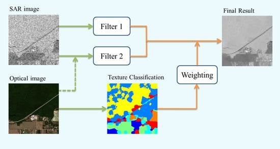
Following the method above, the proposed technique’s block diagram is shown in Figure 3. The original SAR image is filtered by filter 1. Filter 2 is performed with the co-registered optical image, if needed. At the same time, the optical image is split up by SFFCM to obtain the corresponding weights of different regions. Finally, a linear combination is performed to obtain the final SAR image.

3. Experimental Results

In this section, we first compared four filters (PPB, SAR-BM3D, H-WNNM, and GNLM) and then selected several complementary combinations. Next, we chose the best combination as the final output and compared it with other despeckling methods. Contrast experiments were performed on synthetic multiplicative noise images and real SAR images. As shown in Figure 4, we selected six images for the test, including three synthetic (a) and three real SAR images (b), with corresponding co-registration optical images at the bottom. According to [39], we selected representative images with homogeneous regions, complex texture regions, roads, etc. To compare the objective indices of the proposed method with others, we computed the Feature Similarity Index (FSIM) [40] and the Peak Signal-to-Noise Ratio (PSNR) in the synthetic multiplicative noise image. Generally, the larger the PSNR is, the better the image quality will be. FSIM is a number between 0 and 1. The larger FSIM shows that the image structure information preservation is better. The no-reference measure we selected is ENL for real-world SAR images. Generally, a larger ENL indicates a stronger capability of the filter to remove speckle. In addition, we also calculated the ratio images to compare the residual speckle noise.

3.1. Parameter Set

In order to test the sensitivity of the proposed method to parameter C, we further discussed the relationship between the number of clusters and the filtering results. All real-world SAR images and co-registered optical images are from Sentinel 1–2 dataset [41]. The SAR images are obtained by Sentinel-1, the pixel spacing is 20 m, azimuth is 5 m, polarization is VV, and acquisition mode is IW. The optical images are obtained by Sentinel-2, only using bands 4, 3, and 2 (i.e., red, green, and blue channels) to generate RGB images. As shown in Figure 4a, we selected three standard test images with rich homogeneous regions and structures to evaluate the impact of cluster C on the performance of PSNR and FSIM. In these experiments, we contaminated the reference test images with various looks of multiplicative speckle noise (L = 1, 2, 4, 8). We used a combination of SAR-BM3D and GNLM as output (the reason is given later) and set C from 2 to 10 to determine the best value. The curve in Figure 5a shows that PSNR increases significantly when C ranges from 2 to 7 and stabilizes when C is greater than 7. Similarly, the curve in Figure 5b shows that the FSIM values have a clearly increasing tendency when C ranges from 2 to 7. However, in the case of a high number of looks (greater than 7), the values of FSIM are stable. Therefore, we set the cluster number C to 7.

3.2. Comparison of Selected Tools

To acquire a comprehensive understanding of the selected filters, we tested the performance of the four filters. The results are shown in Figure 6. The top lines, from left to right, are noise images (L = 1), PPB, SAR-BM3D, H-WNNM, and GNLM. The bottom row is the corresponding ratio images.

From Figure 6, we can see that PPB and H-WNNM are characterized by excessive smoothing and the loss of many texture details, and PPB also produces some artifacts. On the other hand, SAR-BM3D demonstrates its good capability to preserve textures, but it does not perform well in speckle suppression. GNLM seems to be the best filter, performing well both in homogeneous and complex texture areas, and producing no artifacts. However, in some complex areas, GNLMs’ over-smoothing will lead to the loss of some texture details.

Table 1. FSIM, PSNR, and ENL of the selected despeckling methods.

Methods	FSIM	PSNR	ENL
Single-Look	0.7243	17.63	1.28
PPB	0.8573	25.29	161.69
SAR-BM3D	0.8626	24.86	12.38
H-WNNM	0.7450	21.78	136.24
GNLM	0.8502	26.66	358.58

confirms the visual assessment, where the best values are marked in bold. GNLM is an outperforming filter in despeckling and preserving the main structure details; it also presents the highest values of the PSNR and ENL measurements. The best FSIM is given by SAR-BM3D, which is equal to 0.8626, while the lowest is H-WNNM, which is only 0.7450. The ENL of SAR-BM3D is the lowest, which indicates that it has a poor capability to remove speckle. From the ratio images in the bottom row of Figure 6, we can see GNLM and H-WNNM retain a significant amount of textures, indicating that GNLM and H-WNNM have less capability to preserve texture details. The ratio image of PPB also shows slight texture, which indicates that some texture areas are over-smoothed. SAR-BM3D leaves little texture, which indicates that SAR-BM3D has excellent texture preservation characteristics.

3.3. Comparison of Selected Combinations

Based on the analysis of all the candidate filters in the previous section, we selected the following three combinations for further analysis. They were:

• SAR-BM3D and GNLM (Fusion #1)
• SAR-BM3D and PPB (Fusion #2)
• SAR-BM3D and H-WNNM (Fusion #3)

We combined two complementary filters to overcome their respective shortcomings and achieve the best performance. The experimental results are shown in Figure 7. Considering the very strong noise input, it seems certain that Fusion #1 is providing an encouraging filter quality.

The speckle is suppressed effectively without contaminating the image resolution. In addition, most details are well preserved, even complex textures, without introducing significant artifacts. In contrast, Fusions #2 and #3 cannot suppress speckle effectively. The corresponding ratio images are shown at the bottom of Figure 7. An excellent filter should only remove the injected speckle. Therefore, the ratio image should only contain the speckle without texture. There is an obvious structure leakage in the ratio image of Fusions #2 and #3. Fusion#1 also seems satisfactory. The results of RS1 in Figure 8 confirm these conclusions. It is evident that Fusions #2 and #3 have very limited speckle suppression, and the texture regions are distorted. In contrast, Fusion #1 preserves both detail and linear structure while smoothing the image, and the corresponding ratio image retains less structural information.

In

Table 2. The FSIM, PSNR, and ENL of the candidate combinations. (FSIM, PSNR, and ENL1 are computed on S2; ENL2 is computed on RS1).

Methods	FSIM	PSNR	ENL1	ENL2
Single-Look	0.7076	14.76	1.53	3.57
Fusion #1	0.8356	23.86	384.89	263.20
Fusion #2	0.8109	22.63	92.44	170.91
Fusion #3	0.7758	21.12	138.64	227.08

, we show the numerical results obtained from these images. The Fusion #1 approach seems to show significant performance improvement. Indeed, from the PSNR index, Fusion #1 is much higher (more than 1.2 db) than other combinations. Similar behavior is observed in regards to FSIM and ENL. Fusion #1 provides the best FSIM and ENL with respect to all combinations. Hence, we eventually chose Fusion #1 (SAR-BM3D and GNLM) as the final output based on the above evidence.

3.4. Comparison with Other Despeckling Methods

To further quantitatively and qualitatively evaluate the performance of the proposed method, in this section, all of the images were tested (including synthetic and real SAR images).

All results are compared with previously cited filtering methods (with the addition of the wavelet-contourlet filter (W-C) [42] and Fast Adaptive Non-Local SAR (FANS) [43]), and some regions are enlarged for more accurate analysis. Through visual inspection, we find that in Figure 9, PPB and H-WNNM cause over-smoothing of the image and blur the textures and edges of the image. W-C does not suppress the speckle effectively and produces some artifacts. Although SAR-BM3D preserves image details well, the speckle suppression is limited. FANS produces some artifacts when the noise level is high, mainly due to the recognition of structural errors.

GNLM suppresses speckle well, but blurs the details in complex textured areas. The proposed method preserves these structures while ensuring effective speckle suppression, as demonstrated in the zoomed region. In Figure 10, we can see some structures in the ratio images of W-C, PPB, H-WNNM, and GNLM. Fewer structures exist for the proposed method and FANS, while SAR-BM3D has hardly any structural leakage. The experimental results of another synthetic multiplicative noise image are shown in Figure 11 and Figure 12. Similar to the previous analysis, the proposed method achieves the best balance in preserving the textural structure and speckle suppression.

Objective indices of the selected three synthetic multiplicative noise images are shown in

Table 3. The FSIM, PSNR, and ENL of all filters on the synthesized multiplicative noise images (L = 1, 2, 4, 8).

			L = 1			L = 2			L = 4			L = 8
	Methods	FSIM	PSNR	ENL	FSIM	PSNR	ENL	FSIM	PSNR	ENL	FSIM	PSNR	ENL
	Noisy image	0.7243	17.63	1.28	0.7940	20.78	2.11	0.8534	23.02	3.38	0.9005	25.92	7.87
	W-C	0.7292	21.06	14.62	0.7646	23.12	19.08	0.8000	24.71	26.87	0.8332	26.36	42.74
	PPB	0.8573	25.29	161.69	0.8939	26.89	175.64	0.9195	28.58	243.17	0.9392	30.37	399.28
	SAR-BM3D	0.8626	24.86	12.38	0.8965	26.81	18.87	0.9243	28.89	20.87	0.9477	31.19	43.47
S1	H-WNNM	0.7450	21.78	136.24	0.8032	24.42	154.09	0.8622	27.06	299.54	0.8630	27.63	417.73
	GNLM	0.8502	26.66	358.58	0.8809	27.96	403.74	0.9122	29.22	641.59	0.9364	30.49	765.68
	FANS	0.8762	26.61	73.95	0.9081	28.57	79.96	0.9318	30.42	154.11	0.9506	32.42	197.41
	Proposed	0.8887	27.40	87.77	0.9124	28.80	119.87	0.9308	30.01	142.13	0.9470	31.33	247.33
	Noisy image	0.7076	14.76	1.53	0.7710	17.32	2.39	0.8311	20.15	3.98	0.8811	23.05	7.40
	W-C	0.7541	18.95	3.82	0.7865	20.94	22.25	0.8197	22.61	19.82	0.8522	24.08	27.80
	PPB	0.7342	21.77	192.73	0.8204	23.43	353.06	0.8812	24.92	456.78	0.9115	26.27	885.19
	SAR-BM3D	0.8186	21.63	7.83	0.8596	23.36	16.17	0.8979	25.57	23.24	0.9268	27.57	38.33
S2	H-WNNM	0.6903	17.80	410.32	0.7721	21.43	1522.13	0.8317	24.49	3853.19	0.8374	26.35	5100.64
	GNLM	0.7793	23.32	4641.76	0.8142	24.05	7809.26	0.8706	25.36	4167.69	0.9117	26.50	7353.35
	FANS	0.7861	22.85	67.77	0.8615	24.70	389.37	0.9037	26.62	706.51	0.9295	28.42	479.94
	Proposed	0.8356	23.86	384.89	0.8681	24.95	802.32	0.9017	26.28	693.17	0.9265	27.50	1122.42
	Noisy image	0.6510	19.47	0.96	0.7385	22.20	1.80	0.8174	25.08	3.73	0.8799	28.01	6.77
	W-C	0.7778	25.02	34.89	0.7923	26.63	41.51	0.8141	27.75	62.34	0.8392	28.88	88.23
	PPB	0.8102	28.34	131.32	0.8524	29.86	188.35	0.8903	31.30	226.18	0.9203	32.59	241.50
	SAR-BM3D	0.8405	27.41	10.12	0.8768	29.16	12.57	0.9116	31.27	18.24	0.9359	33.31	28.60
S3	H-WNNM	0.7081	24.59	1467.09	0.7545	27.34	2285.85	0.8098	29.69	2540.52	0.8250	30.57	2052.38
	GNLM	0.8340	30.14	190.29	0.8474	30.92	297.08	0.8757	31.94	264.05	0.9118	33.27	233.44
	FANS	0.8308	29.19	121.25	0.8723	31.03	271.44	0.9046	32.69	185.47	0.9328	34.42	130.82
	Proposed	0.8649	30.47	183.72	0.8818	31.53	196.25	0.9013	32.59	191.62	0.9261	33.81	139.86

. It can be seen that the FSIM and PSNR of the proposed method are nearly optimal when L is less than 4, and especially when L equal to 1 (the most challenging case). W-C and H-WNNM provide poor results, as shown in Table 3. PPB, SAR-BM3D, GNLM, and FANS obtain good objective values, but they are lower than the proposed method. This means the proposed method can obtain good despeckling results for images corrupted by very strong speckle noise.

However, when the number of looks is high (i.e., the noise level is low), SAR-BM3D and FANS perform quite well. The main reason is that when the noise level is low, the filtering results of SAR-BM3D and FANS do not introduce excessive residues and artifacts, respectively. Regarding ENL, GNLM and H-WNNM maintain nearly the highest ENL. PPB and FANS can obtain better ENL values than W-C and SAR-BM3D. Although the ENL of the proposed method is not the highest, it exceeds PPB and FANS. This indicates that the proposed method can adequately suppress speckle in homogeneous regions.

These results are even more important for real-world SAR images than for synthetic ones. The values of ENL of the three selected real-world SAR images are shown in

Table 4. The ENL and run times (in seconds) of all filters on real-world SAR images.

Methods	RS1	RS2	RS3	Time (s)
Noisy image	3.15	13.27	26.60	/
W-C	15.66	42.19	195.06	18
PPB	434.64	459.31	1137.34	23
SAR-BM3D	55.42	24.48	59.56	32
H-WNNM	5352.23	643.13	2411.27	138
GNLM	338.71	1417.92	5127.57	89
FANS	166.96	62.79	215.82	16
Proposed	263.20	589.10	2435.91	125

. H-WNNM and GNLM are the two filters with the strongest speckle noise suppression capability, while W-C and SAR-BM3D are the worst. PPB provides better performance than FANS.

Since the proposed method combines the features of GNLM and SAR-BM3D, the ENL is lower than that for GNLM. However, it is better than for PPB and FANS, demonstrating that the proposed method guarantees adequate speckle suppression.

Visual inspection is necessary for a solid evaluation. In Figure 13, we show the results of the real-world SAR image RS1 and the zooming area of interest. As shown in Figure 13, PPB, H-WNNM, GNLM, and FANS do not completely preserve texture details. PPB and FANS also produce ghost artifacts. W-C has limited speckle suppression capability, and it produces some artifacts. SAR-BM3D faithfully preserves the texture details, but it retains too much speckle noise. The proposed method shows good performance, not only in effective speckle suppression, but also in the preservation of the most textural details. The ratio images of the proposed method in Figure 14 also contain the least structures. The despeckling results for real-world SAR images RS2 and RS3 are shown in Figure 15, Figure 16, Figure 17 and Figure 18, respectively. It is reconfirmed that the proposed method preserves the edge and image details while removing speckle.

The executable codes of the compared methods can be downloaded from the authors’websites (http://www.math.u-bordeaux1.fr/~cdeledal/ppb; http://www.grip.unina.it/web-download.html; https://github.com/csjunxu/WNNM_CVPR2014; https://github.com/grip-unina/GNLM) accessed on 15 December 2020, and the parameters were set as recommended. All the experiments were run in MATLAB R2017a on a desktop computer with an Intel Pentium 2.80 GHz CPU and 8GB memory. In Table 4, it is shown that the processing speed of FANS is higher than the other competing algorithms. W-C, PPB, and SAR-BM3D also achieve faster speed. H-WNNM takes the longest time. The proposed method uses two different filtering strategies; therefore, it does not yield superior results in terms of processing time. In the future, we will study how to reduce the complexity of the algorithm in order to reduce the running time.

4. Discussion

In this study, two complementary filters are combined for despeckling, and the weights are allocated from an offline database based on GLCM learning. Since a single filter has different advantages and disadvantages, the proposed method can combine these advantages and overcome the disadvantages. Synthetic and real-world SAR images are used in the experiment. The purpose of using synthetic multiplicative noise images is to obtain rich objective indexes; this is helpful for us to evaluate the performance of the proposed method.

The experimental results compared with other filters show that the proposed method exhibits nearly the highest FSIM and PSNR at a high noise level (L less than 8). Although the ENL of the proposed method is not the highest, the visual inspection proves that the noise suppression capability of the proposed method is better. We observe similar results described previously in real-world SAR images, and the proposed method achieves an optimal balance between preserving image edges and textures and suppressing speckle. However, when the noise level is low, FANS achieves better filtering results. Perhaps when L is more than 4, we could add FANS as the third combination.

In the future, we will consider how to better solve this problem, and we will optimize the code scheme to reduce the processing time of the proposed method. Moreover, the probability of the incorrect assignment of weights can be reduced by increasing the training data. This would help reduce the generation of artifacts.

5. Conclusions

We propose a new weighted combination method based on block classification for the two most advanced SAR image despeckling methods. By clustering the co-registered optical images with SFFCM, similar blocks are obtained and weights are assigned to two different filters. The weights are set empirically by the feature images of the GLCM. Two complementary combinations of filters can produce better results. The two complementary filters are selected through experimental analysis of the existing filter schemes. The experimental results show that our proposed method provides the highest objective indices under very strong noise contamination when compared to other methods. Strong speckle suppression is observed, together with a faithful preservation of details. Other methods may show insufficient or excessive speckle rejection. Experiments on real-world SAR images are likewise encouraging, as the proposed method does an excellent job of texture preservation and artifact reduction. For SAR images with low noise level, although our method achieves good despeckling results, FANS seems to obtain even better results.

Since a large part of our scheme relies on the co-registration of optical images, the current research is not fully automated. Future work may resort to deep-learning methods to improve this issue. We hope that more people will invest in this research. Another important drawback of our method is its complexity. Simplifying this method is also a direction for our future research efforts.