Satellite-Derived Photosynthetically Available Radiation at the Coastal Arctic Seafloor

Abstract

Climate change has affected the Arctic Ocean (AO) and its marginal seas significantly. The reduction of sea ice in the Arctic region has altered the magnitude of photosynthetically available radiation (PAR) entering the water column, impacting primary productivity. Increasing cloudiness in the atmosphere and rising turbidity in the coastal waters of the Arctic region are considered as the major factors that counteract the effect of reduced sea ice on underwater PAR. Additionally, extreme solar zenith angles and sea-ice cover in the AO increase the complexity of retrieving PAR. In this study, a PAR algorithm based on radiative transfer in the atmosphere and satellite observations is implemented to evaluate the effect of these factors on PAR in the coastal AO. To improve the performance of the algorithm, a flag is defined to identify pixels containing open-water, sea-ice or cloud. The use of flag enabled selective application of algorithms to compute the input parameters for the PAR algorithm. The PAR algorithm is validated using in situ measurements from various coastal sites in the Arctic and sub-Arctic seas. The algorithm estimated daily integrated PAR above the sea surface with an uncertainty of 19% in summer. The uncertainty increased to 24% when the algorithm was applied year-round. The PAR values at the seafloor were estimated with an uncertainty of 76%, with 36% of the samples under sea ice and/or cloud cover. The robust performance of the PAR algorithm in the pan-Arctic region throughout the year will help to effectively study the temporal and spatial variability of PAR in the Arctic coastal waters. The calculated PAR data are used to quantify the changing trend in PAR at the seafloor in the coastal AO with depth < 100 m using MODIS-Aqua data from 2003 to 2020. The general trends calculated using the pixels with average PAR > 0.415 mol m${}^{-2}$ day${}^{-1}$ at the seafloor during summer indicate that the annual average of PAR entering the water column in the coastal AO between 2003 and 2020 increased by 23%. Concurrently, due to increased turbidity, the attenuation in the water column increased by 22%. The surge in incident PAR in the water column due to retreating sea ice first led to increased PAR observed at the seafloor (∼12% between 2003 and 2014). However, in the last decade, the rapid increase in light attenuation of the water column has restricted the increase in average annual PAR reaching the bottom in the coastal AO.

1. Introduction

In recent decades, the sea-ice cover in the Arctic Ocean (AO) has significantly declined in extent, thickness, and volume [1]. The lack of sea ice affects flora and fauna [2] and the traditional means of transportation and subsistence for coastal communities [3]. Light availability in the water column has changed significantly, with seasonal climatic oscillations affecting the growth of primary producers [4,5,6]. The light utilized by autotrophs for photosynthesis lies within the spectral range of 400 to 700 nm, called Photosynthetically Available Radiation (PAR) [7]. PAR acts as a critical indicator for predicting the health and production of autotrophs and the evolution of the marine ecosystem. Accurately estimating PAR availability has important implications in estimating the primary production, carbon budget, ocean acidification, water quality and heat budget in the water column [8,9,10,11,12,13].

The reduction in sea-ice thickness and spatial extent of the sea-ice cover has resulted in the increased magnitude of daily PAR entering the water surface in the AO [14,15,16]. Still, the lack of light availability due to long nights in winters, and sea-ice cover in the Arctic region makes PAR an essential environmental parameter of the Arctic ecosystem. Furthermore, increasing cloudiness and water turbidity due to increased coastal erosion and permafrost melting can counteract the increase in PAR and may lead to negative trends of PAR at local scale [14,17,18]. These factors affect the magnitude of light reaching the seafloor in the coastal AO, impacting the growth of macrophytes, especially kelp [19]. Macrophytes are key contributors to coastal primary production in the AO, provide important habitat, food sources and nursery for many animals (invertebrates, fish and sea birds) and are potential exporters of carbon to the deep ocean [20]. Increasing light in the water column due to sea-ice retreat and the contrasting role of increasing coastal turbidity has been suggested to counteract the increase in macrophytes [21]. Nevertheless, PAR is expected to increase in coastal waters, favouring the net growth of macrophytes along many Arctic coastlines [22,23,24].

In a previous study, Bélanger et al. [14] observed a 3% decrease in daily PAR reaching the ocean surface in the pan-Arctic region between 1998 and 2009 due to increasing cloudiness. Recently, Laliberté et al. [25] reported a similar decline in PAR reaching the ocean surface with a 2.3% reduction between 2000 and 2016. Yet, the PAR penetrating the sea surface in the Arctic region has increased significantly due to the shrinking of the sea-ice cover [6,14,16,26]. Meanwhile, melting ice over the land, glaciers, and rivers brings a substantial amount of sediments and dissolved organic matter to the littoral zone. This increase in terrestrial input combined with increased wind-induced sediment re-suspension over the ice-free coastal AO have increased the turbidity in coastal water, thereby limiting primary production [19]. Conversely, the increased light and nutrients from the riverine discharge resulted in a steady increase in primary production, particularly in the interior shelves of the AO [6]. Therefore, quantifying the variability in PAR can help understand the impacts of global warming on primary production and health of the coastal ecosystems.

Monitoring the AO is difficult due to lack of accessibility and expensive/labour-extensive field programs; thus, remote sensing can play an important role. Earth Observation (EO) satellites provide a synoptic view of the general spatial and temporal trends of PAR at the global [27], and regional scales [14,25]. Nevertheless, the dynamic climate variables at high latitude (such as winds, clouds, and sea-ice cover) coupled with higher solar zenith angle increases the complexity of PAR retrieval using remote sensing data [28]. The standard algorithm used by NASA Ocean Biology Processing Group (OBPG) (hereafter, OBPG algorithm) to calculate PAR just above the sea surface (PAR($0^{+}$)) from satellite data [29,30] performs well with uncertainty less than 20% in daily PAR($0^{+}$) [31]. However, it has limited application in the ice-covered polar waters as this algorithm is not designed to work in the presence of sea ice [32,33]. Besides incoming PAR, PAR reaching the seafloor (PAR($z_{\mathrm{b}}$)) can also be estimated from satellite observations using water column attenuation parameterization. Gattuso et al. [34] used the OBPG algorithm to estimate PAR at the ocean surface and Morel [35] to calculate downwelling diffused attenuation coefficient for PAR ($K_{\mathrm{d}}^{\mathrm{PAR}}$) to make the first assessment of PAR($z_{\mathrm{b}}$) at the global scale, including in the Arctic shelves. This PAR($z_{\mathrm{b}}$) estimation by Gattuso et al. [34] was upgraded with higher spatial resolution bathymetry and better $K_{\mathrm{d}}^{\mathrm{PAR}}$ by Gattuso et al. [36]. However, $K_{\mathrm{d}}^{\mathrm{PAR}}$ used in these studies is based on Chlorophyll-a concentration ($C_{\mathrm{Chl}-a}$), and the accuracy of $C_{\mathrm{Chl}-a}$ retrieval from remote sensing in coastal waters remains uncertain, as reported by Antoine et al. [37] in the Beaufort Sea. Therefore, more accurate surface PAR and $K_{\mathrm{d}}^{\mathrm{PAR}}$ are essential for a better estimate of PAR($z_{\mathrm{b}}$) in coastal Arctic waters.

Beside bathymetry, the other major components essential for the calculation of PAR reaching the seafloor are (1) PAR calculated just below the sea surface (PAR($0^{-}$)) and (2) $K_{\mathrm{d}}^{\mathrm{PAR}}$ to compute the attenuation of PAR($0^{-}$) in the water column. However, in polar waters covered with sea ice, sea-ice cover and transmittance also play an important role in the computation of underwater PAR. In general, the satellite-derived PAR is calculated just above the sea surface (PAR($0^{+}$)). The major factor affecting the incident PAR($0^{+}$) is the atmospheric transmission of light in the visible bands. Therefore, the magnitude of incident PAR($0^{+}$) is mainly governed by the scattering and absorption by the atmospheric gases (such as ${\mathrm{N}}_2$, ${\mathrm{O}}_2$ and ${\mathrm{O}}_3$), aerosols, clouds, surface albedo, and the direction of the incident light (represented by solar zenith angle, ${\theta }_0$) [27]. At higher ${\theta }_0$, a significant amount of light gets specularly reflected from the sea surface [38] leading to significantly lower PAR($0^{-}$) compared to PAR($0^{+}$). Therefore, it is essential to implement specialized methods to accurately estimate PAR($0^{-}$). Considering these necessities, Bélanger et al. [14] employed the Santa Barbara DISORT Atmospheric Radiative Transfer (SBDART) model [39] to estimate PAR($0^{+}$) and PAR($0^{-}$) at extreme solar zenith angles under changing climate variables (such as clouds, ozone layer, sea-ice cover). Laliberté et al. [32] (hereafter, LBF2016 algorithm) upgraded this algorithm by including the variability of mean surface albedo in the spectral range of PAR (${\overline{\alpha }}_{\mathrm{s}}$), increasing the accuracy of the PAR algorithm in the presence of sea ice. The cloud and ozone parameters used as input for these studies were provided by the International Satellite Cloud Climatology Project (ISCCP) at very low spatial resolution (280 km) [40]. Given that ISCCP data stopped in 2009, the coarse resolution of this dataset and the requirement for a continuous climate-compatible time series (i.e., free of sensor artifact), most of the input parameters were derived using a single sensor, i.e., the Moderate Resolution Imaging Spectroradiometer (MODIS) onboard Aqua (2002-present). The second essential parameter, $K_{\mathrm{d}}^{\mathrm{PAR}}$, can be estimated using the downwelling diffused attenuation coefficient at 490 nm ($K_{\mathrm{d}}$(490 nm)) [41], and Lee et al. [42] can be used to calculate $K_{\mathrm{d}}$ at a wavelength ($\lambda$) using satellite data with reasonable accuracy, even in the Arctic region [43]. Estimation of $K_{\mathrm{d}}\left(\lambda \right)$ in coastal waters from satellite data remains challenging due to increased uncertainty in the atmospheric correction of ocean colour data [28,44].

The main goal of this study was to upgrade and validate the LBF2016 model to assess daily PAR entering the water column and reaching the seafloor. Although the model can be used to evaluate primary production in the water column, here we focused on PAR received by the benthic component of the marine ecosystem, which has received less attention than the water column over the last decade [6,14,45,46], but is expected to play a major role along the Arctic coast in response to climate change [20,22]. The radiative transfer model to estimate daily integral PAR at the sea surface (especially PAR($0^{-}$)) is efficient while considering the merits and limitations of satellite-based retrieval of PAR in the sea-ice covered coastal waters of the AO. Therefore, in the present study, two look-up tables (LUTs) with solar zenith angle (${\theta }_0$), ozone optical thickness (${\mathsf{\tau }}_{\mathrm{oz}}$), cloud optical thickness (${\mathsf{\tau }}_{\mathrm{c}}$) and mean surface albedo in the spectral range of PAR (${\overline{\alpha }}_{\mathrm{s}}$) as variables are computed using the SBDART model as described by LBF2016 for PAR($0^{+}$) and PAR($0^{-}$). Then different methods are applied to either compute or retrieve the four input parameters for these LUTs from various satellite sources. The efficacy of the other important component for PAR($z_{\mathrm{b}}$) estimation, $K_{\mathrm{d}}\left(\lambda \right)$, can be improved significantly by using atmospheric correction especially designed for coastal waters. Therefore, the spectral shape parameter (SSP) based atmospheric correction method [47] is used to derive the aerosol optical thickness (${\mathsf{\tau }}_{\mathrm{a}}$) and remote-sensing reflectance used as input for the $K_{\mathrm{d}}$ model of Lee et al. [42]. The estimation/retrieval of input parameters for the LUTs from satellite data using SSP atmospheric correction algorithm [47], which is designed especially for coastal water applications, and more accurate computation of $K_{\mathrm{d}}\left(\lambda \right)$ using Lee et al. [42] increases the robustness of the algorithm substantially. To assess the performance of the PAR algorithm, long-term in situ data from stations/moorings at the surface and seafloor from different coastal regions in the AO are used. Additionally, the result from the present study is compared with the PAR($z_{\mathrm{b}}$) estimated by Gattuso et al. [36], and a general trend of PAR($z_{\mathrm{b}}$) between 2003 and 2020 in the pan-Arctic domain is computed for the coastal waters of the AO.

In the next section (Section 2), we provide the details of the satellite and in situ data used for the validation of the PAR model. Section 3 deals with the details of the method used to compute PAR values at surface and bottom. As stated above, the present study employed the LUTs derived from the SBDART model to compute PAR($0^{+}$) and PAR($0^{-}$). To increase the robustness of the model, the input parameters (${\theta }_0$, ${\mathsf{\tau }}_{\mathrm{oz}}$, ${\mathsf{\tau }}_{\mathrm{c}}$ and ${\overline{\alpha }}_{\mathrm{s}}$) for the LUTs are also computed using the full-resolution MODIS-Aqua data (Level 1A; Top of atmosphere radiance). This section also includes the assumptions and methods used to compute the input parameters. Section 4 contains the evaluation of the method, demonstrating the effectiveness of the assumptions made to compute input parameters in Section 3. A brief description of the pan-Arctic trends in PAR in recent decades is also presented in this section as an example of application of the method. Finally, a summary of the results and conclusion is given in the last section (Section 5) of the article.

2. Satellite and In Situ Data

2.1. Satellite Data

Algorithms based on ocean colour data from space-borne sensors can help estimate PAR($0^{+}$) with good accuracy and provide synoptic coverage of the AO with high temporal resolution. However, the gaps in satellite observations can degrade the quality of standard satellite-derived daily PAR [25,27,32]. Multiple overpasses of polar-orbiting satellites over the Arctic region within a day can fill the gaps in the observations and reduce the uncertainty in the estimation of PAR due to variation of clouds [25]. Therefore, the MODIS-Aqua data are used in the present study to calculate PAR at surface (PAR($0^{+}$) and PAR($0^{-}$) and used satellite derived $K_{\mathrm{d}}^{\mathrm{PAR}}$ to compute PAR($z_{\mathrm{b}}$). MODIS-Aqua has a wide swath (2330 km) with a moderate spatial resolution of 1 km at nadir, providing continuous coverage of PAR for the pan-Arctic region. Moreover, the surface PAR estimated using MODIS-Aqua data has low uncertainty over large timescales [30].

The MODIS-Aqua L1A data were downloaded from the NASA Ocean Biology Distributed Active Archive Center (OBDAAC, oceancolor.gsfc.nasa.gov, 16 September 2020). The L1A images were processed in SeaDAS v7.5 by implementing the SSP aerosol correction algorithm of Singh et al. [47] to calculate atmospheric and oceanic parameters (such as aerosol optical thickness (${\mathsf{\tau }}_{\mathrm{a}}\left(\lambda \right)$) and surface reflectance (${\rho }_{\mathrm{s}}\left(\lambda \right)$)) required for the estimation of PAR at surface and seafloor and $K_{\mathrm{d}}\left(\lambda \right)$. MODIS data are also used to compute ${\mathsf{\tau }}_{\mathrm{c}}$ and ${\overline{\alpha }}_{\mathrm{s}}$. The near real-time sea-ice concentration ($C_{\mathrm{ice}}$) was processed using the NASA Team algorithm [48] at 25 km × 25 km spatial resolution. This processed $C_{\mathrm{ice}}$ was acquired from the National Snow and Ice Data Center (NSIDC) [49,50] via NASA OBDAAC and re-sampled corresponding to the spatial resolution of MODIS-Aqua. Daily ${\mathsf{\tau }}_{\mathrm{oz}}$ was obtained from Earth Probe (EP) Total Ozone Mapping Spectrometer (TOMS) [51] at 1.0° × 1.25° spatial resolution and the Ozone Monitoring Instrument (OMI onboard Aura) [52] at 1.0° × 1.0° spatial resolution through NASA OBDAAC (Figure 1). Finally, ETOPO1 [53] was used for bathymetry as it matches the spatial resolution of MODIS-Aqua (Figure 2).

2.2. In Situ Data

The accuracy of the PAR obtained by the algorithm was tested using in situ data collected at various Arctic and sub-Arctic locations. These data were recorded at different coastal locations mostly spread through the western hemisphere, located at varying latitudes and, therefore, providing a wide range on environments to test the performance of the PAR algorithm.

Table 1. Details of the in situ data used to validate PAR.

Region	Name	Latitude (°N)	Longitude (°E)	Measurement Depth (m)	Period		Source
					From	To
James Bay	C33-JB	53.746	−79.121	$0^{+}$	28 June 2019	23 August 2019	UQAR
	V31-JB	52.360	−78.614	$0^{+}$	3 July 2019	20 August 2019
Isfjorden	ISA	78.223	15.652	$0^{+}$	19 February 2019	16 August 2020	UNIS
	IAF	78.233	15.689	1.2	17 June 2020	4 October 2020
Stefansson Sound	Endeavor	70.353	−147.961	$0^{+}$	26 July 2002	9 August 2006	[54]
	MPI	70.353	−147.961	$0^{+}$	26 July 2007	13 July 2018
	DS11	70.322	−147.578	6.1	25 July 2004	14 July 2018
	E1	70.314	−147.732	4.4	25 July 2004	14 July 2018
	E2	70.318	−147.715	4.3	22 July 2005	3 August 2006
	L1	70.289	−147.613	5.5	31 August 2014	14 July 2018
	W1	70.370	−147.873	6.0	27 August 2014	8 September 2014
	W2	70.370	−147.859	6.2	22 July 2005	9 August 2006
	W3	70.376	−147.794	6.6	30 July 2016	16 September 2017

UQAR = Université du Québec à Rimouski, UNIS = University Center in Svalbard.

lists the location of the stations along with the duration in which the data were recorded.

It is difficult to install and maintain stations/moorings in the Arctic region, and hence, data from some stations were collected during summer only. These include the data from two stations (C33-JB and V31-JB) installed on small islands (50–100 m wide) in James Bay (located in the south of Hudson Bay in Canada) and one station (Endeavor) installed in the Stefansson Sound situated in the Beaufort Sea at the northern coast of Alaska, USA. These stations are located in the sub-Arctic (James Bay, latitude ∼53°N) and the Arctic (latitude ∼70°N) and cover two distinct periods (Table 1 and Figure 2).

Furthermore, there were two stations, MPI (in Stefansson Sound) and ISA on the roof of the University Center in Svalbard (UNIS) (Longyearbyen, Svalbard), that have recorded PAR($0^{+}$) throughout the year. The station at UNIS (ISA) is located on land, but the algorithm used in the present study is developed for marine applications. The significant difference in the surface albedo of land when compared with water would lead to higher uncertainty in the estimation of PAR at land. Besides, potential adjacency and multiple scattering effects between the surface and the lower atmosphere in the presence of brighter land surface could yield higher PAR values if compared to PAR estimated over a water surface [32].

Seven moorings deployed underwater (almost near the seafloor) in the Stefansson Sound, and one PAR sensor (IAF) deployed at 1.2 m depth (the total depth of the statiion is 13 m) close to the innermost river catchment area of Adventfjorden were used to validate the satellite-derived PAR($z_{\mathrm{b}}$).

Sensitivity of In Situ Sensors

The PAR sensors used in the present study are manufactured by different companies and have different sensitivities. Moreover, they are deployed in extreme environmental conditions affecting the accuracy of these sensors. The PAR sensors are deployed in cold environments for long periods of time with varying amounts of sunlight ranging from minimum (∼zero) during the polar night and maximum during the polar day. According to the manufacturer, the sensors have an uncertainty of $\pm 5\%$ along with a temperature-induced uncertainty of $\pm 0.15\%$ per °C to the in situ PAR recorded by LICOR LI-193 and LICOR SPQA-193 sensors at all the sites except ISA. At ISA, HOBO S-LIA-M003 records in situ PAR with an uncertainty of $\pm 5\%$. However, this PAR sensor has a significantly higher drift of $\pm 0.75\mathsf{\mu }\mathrm{mol}{\mathrm{m}}^{-2}{\mathrm{s}}^{-1}{}^{\circ }{\mathrm{C}}^{-1}$ at 25 °C due to a change in temperature.

The uncertainty in PAR recorded by these sensors in good light conditions is ≤5%, fulfilling the uncertainty requirements defined for field measurement of radiometric quantities by IOCCG [55]. However, during the low light conditions in winter, and when the temperature reaches well below 0 °C the PAR values recorded by these in situ sensors drifts significantly from the actual value. The uncertainty in the PAR recorded from LICOR sensors increase by another $\pm 0.15\%$ per °C relative to sensor calibration (25 °C), yielding an uncertainty of $\pm 8.75\%$ at 0 °C [56]. At the same time, the in situ PAR recorded by HOBO S-LIA-M003 can deviate by $\pm 18.75\mathsf{\mu }\mathrm{mol}{\mathrm{m}}^{-2}{\mathrm{s}}^{-1}$ at 0 °C adding to the standard uncertainty of $\pm 5\%$. Therefore, it is essential to consider the effect of sensitivity of the PAR sensors deployed in low light and cold conditions (especially, MPI and ISA) on validation of the PAR values computed in the present study.

Due to the variation in the sensitivity of these sensors with respect to temperature and illumination conditions, the data from all these sensors may have a bias. The PAR sensors deployed at ISA and MPI collected data throughout the year, including low light conditions leading to polar night. These sensors also recorded PAR at sub-zero air temperatures, which would have increased the uncertainty in the PAR values recorded in these conditions. The uncertainty and bias vary for every in situ sensor. If the data from all sensors is used altogether to validate the model output, then the uncertainty in the in situ observations and the uncertainty of the model observations could not be resolved efficiently. Therefore, the data from these sensors were used separately for validation to avoid misrepresentation of uncertainty and bias of the in situ instrument with model uncertainty.

The data from PAR sensors are grouped in four different categories based on the deployment illumination conditions and temperature range. The four groups are (1) PAR sensors deployed during summer (C33-JB, V31-JB and Endeavor), (2) PAR sensor deployed at Stefansson Sound (MPI) throughout the year, (3) PAR sensor installed at Isfjorden (ISA) collecting PAR continuously for more than one year, and (4) the underwater moorings deployed in summer at the Stefansson Sound and Adventfjorden (IAF).

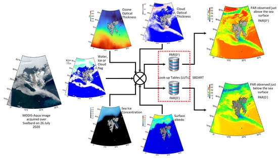
3. The PAR Algorithm

The LUTs used to calculate PAR were computed using the SBDART model as detailed in LBF2016. These LUTs are based on the variation in (1) Solar zenith angle (${\theta }_0$) denoting the direction of the incident PAR, (2) Ozone optical thickness (${\mathsf{\tau }}_{\mathrm{oz}}$) representing the absorption of PAR by ${\mathrm{O}}_3$ gas, (3) Cloud optical thickness (${\mathsf{\tau }}_{\mathrm{c}}$) quantifying the effect of clouds on PAR reaching the surface, and (4) Mean surface albedo in the spectral range of PAR (${\overline{\alpha }}_{\mathrm{s}}$) denoting the fraction of PAR reflected by the surface. As stated earlier, Bélanger et al. [14] and LBF2016 used ${\mathsf{\tau }}_{\mathrm{c}}$ provided by ISCCP. Surface albedo, ${\overline{\alpha }}_{\mathrm{s}}$, was assumed constant by Bélanger et al. [14], whereas LBF2016 (their Equation (2); and Equation (4) below) took a value that depended on sea-ice concentration ($C_{\mathrm{ice}}$) derived from passive microwave and the ice albedo for different phases of sea ice from Perovich et al. [57] (see also Laliberté et al. [25]). The present study aims to calculate ${\mathsf{\tau }}_{\mathrm{c}}$ and ${\overline{\alpha }}_{\mathrm{s}}$ for each pixel at a much finer spatial resolution than in previous works, which had a spatial resolution of 280 km and 25 km for ${\mathsf{\tau }}_{\mathrm{c}}$ and ${\overline{\alpha }}_{\mathrm{s}}$, respectively. Therefore, both ${\mathsf{\tau }}_{\mathrm{c}}$ and ${\overline{\alpha }}_{\mathrm{s}}$ are now retrieved from MODIS data directly. To do so, we defined a flag ($f_{\mathrm{WIC}}$) to identify pixels containing water, sea ice or cloud and treated them accordingly. $f_{\mathrm{WIC}}$ marks the MODIS pixels either as water, sea ice or cloud (fractional cloud or sea-ice cover is assumed to be unity). The detailed descriptions for estimation of $f_{\mathrm{WIC}}$, ${\overline{\alpha }}_{\mathrm{s}}$, ${\mathsf{\tau }}_{\mathrm{c}}$ and PAR are described below.

3.1. Water, Ice, or Cloud Flag ($f_{\mathrm{WIC}}$)

The sea ice, snow and clouds are white surfaces with similar spectral features in the visible bands. Therefore, it is necessary to segregate sea ice or snow (hereafter referred to as sea ice for simplicity) from cloud pixels to avoid miscalculation of atmospheric and surface parameters. The water, sea ice or cloud flag ($f_{\mathrm{WIC}}$) marks the pixel containing water and differentiates between thick clouds and sea ice. However, at 1 km spatial resolution, $f_{\mathrm{WIC}}$ will flag the pixel based on the dominant constituent in the pixel. For example, if the pixel is mainly filled with sea ice, it will be flagged as sea ice, even though it may contain water and clouds. At the higher spatial resolution, the $f_{\mathrm{WIC}}$ can misidentify whitecaps as clouds or sea ice; however, whitecaps are spatially averaged in 1 km pixels, diminishing their effect on the computed indices [58].

Sea ice is significantly brighter than water (Figure 3a); therefore, it can be easily distinguished. But the presence of clouds increase the complexity in the detection of sea ice [59]. Markus et al. [60] found that sea ice and water can be differentiated using a threshold value in the blue spectral band (${\lambda }_{\mathrm{b}}$). However, in the coastal waters, suspended particulate matter (SPM) or phytoplankton (high $C_{\mathrm{Chl}-a}$) may increase the reflectance at ${\lambda }_{\mathrm{b}}$ leading to uncertainty in sea-ice detection. For example, the elevated signals due to coccolithophore blooms to the southeast of Svalbard (Figure 3a) may result in these pixels being flagged as sea ice. Wang and Shi [61] found a remedy to this problem by employing the blue-green reflectance ratio, ${\mathcal{Q}}_{\mathrm{gb}}={\rho }_{\mathrm{s}}\left({\lambda }_{\mathrm{g}}\right)/{\rho }_{\mathrm{s}}\left({\lambda }_{\mathrm{b}}\right)$, to separate the sea-ice pixels from the turbid coastal water pixels. Moreover, the low albedo of sea ice can be distinguished from clouds using the reflective near-infrared band (${\lambda }_{\mathrm{n}}$) and shortwave infrared band (${\lambda }_{\mathrm{s}}$), which are sensitive to temperature (Figure 3b) [62]. The 859 nm and 2130 nm bands of MODIS-Aqua are used as ${\lambda }_{\mathrm{n}}$ and ${\lambda }_{\mathrm{s}}$, respectively.

The normalised difference indices ($\mathcal{N}$) are calculated using (${\lambda }_{\mathrm{g}}$, ${\lambda }_{\mathrm{b}}$) and (${\lambda }_{\mathrm{n}}$, ${\lambda }_{\mathrm{s}}$) to capture the difference in the spectra more effectively.

$${\mathcal{N}}_{\mathrm{gb}}=\frac{{\rho }_{\mathrm{s}}\left({\lambda }_{\mathrm{g}}\right)-{\rho }_{\mathrm{s}}\left({\lambda }_{\mathrm{b}}\right)}{{\rho }_{\mathrm{s}}\left({\lambda }_{\mathrm{g}}\right)+{\rho }_{\mathrm{s}}\left({\lambda }_{\mathrm{b}}\right)}$$

(1)

$${\mathcal{N}}_{\mathrm{ns}}=\frac{{\rho }_{\mathrm{s}}\left({\lambda }_{\mathrm{n}}\right)-{\rho }_{\mathrm{s}}\left({\lambda }_{\mathrm{s}}\right)}{{\rho }_{\mathrm{s}}\left({\lambda }_{\mathrm{n}}\right)+{\rho }_{\mathrm{s}}\left({\lambda }_{\mathrm{s}}\right)}$$

(2)

Finally, the shortwave-infrared (SWIR) band and near-infrared (NIR) bands are used to distinguish sea ice and clouds. The clouds have significantly higher radiance values in SWIR as compared to sea ice that is almost black due to high ice absorption coefficient in this spectral domain (Warren [63], Figure 3b). Moreover, clouds remain bright in NIR resulting in lower gradient between radiance at SWIR and NIR for clouds as compared to sea ice. Therefore, the projection of the slope between ${\rho }_{\mathrm{s}}\left({\lambda }_{\mathrm{n}}\right)$ and ${\rho }_{\mathrm{s}}\left({\lambda }_{\mathrm{s}}\right)$ on the y-axis ($\mathfrak{n}$) of the $\lambda$ vs. ${\rho }_{\mathrm{s}}$ plot can used to distinguish between the clouds and sea ice.

$$\mathfrak{n}=\frac{{\rho }_{\mathrm{s}}\left({\lambda }_{\mathrm{s}}\right){\lambda }_{\mathrm{n}}-{\rho }_{\mathrm{s}}\left({\lambda }_{\mathrm{n}}\right){\lambda }_{\mathrm{s}}}{{\lambda }_{\mathrm{n}}-{\lambda }_{\mathrm{s}}}$$

(3)

The $f_{\mathrm{WIC}}$ (shown in Figure 3d) is calculated using the following steps:

Step 1:

If ${\theta }_0>{83}^{\circ }$, then there will not be enough light to calculate $f_{\mathrm{WIC}}$. Else, the pixel is assumed to contain water, $f_{\mathrm{WIC}}$ = water.

Step 2:

The higher $\mathfrak{n}$ and lower ${\mathcal{N}}_{\mathrm{gb}}$ represent clouds that are almost spectrally flat in the visible region. Therefore, when $\mathfrak{n}>0.1$ and ${\mathcal{N}}_{\mathrm{gb}}<0.1$, the pixel is assumed to contain cloud, $f_{\mathrm{WIC}}$ = cloud.

Step 3:

The higher ${\mathcal{N}}_{\mathrm{ns}}$ shows that ${\rho }_{\mathrm{s}}\left({\lambda }_{\mathrm{n}}\right)$ is significantly higher than ${\rho }_{\mathrm{s}}\left({\lambda }_{\mathrm{s}}\right)$, which is more sensitive to temperature [62], pointing towards the presence of sea ice in the pixel. Furthermore, the effect of turbidity on ${\mathcal{N}}_{\mathrm{ns}}$ can be minimized using ${\mathcal{Q}}_{\mathrm{gb}}$. Hence, if ${\mathcal{N}}_{\mathrm{ns}}/{\mathcal{Q}}_{\mathrm{gb}}>0.6$ and ${\rho }_{\mathrm{s}}\left({\lambda }_{\mathrm{b}}\right)>0.12$, the pixel is assumed to contain ice, $f_{\mathrm{WIC}}$ = ice.

A pixel flagged as cloud may contain water or sea ice, which has implications for the estimation of PAR. Therefore, pixels flagged as clouds are treated separately while calculating the input parameters for the LUTs along with the daily integrated PAR values, as described in Section 3.2.3. $f_{\mathrm{WIC}}$ plays an essential role in coastal waters (Figure 3), especially in the summer months when $C_{\mathrm{ice}}$ acquired from passive microwaves at low spatial resolution has low accuracy due to melting sea ice [64].

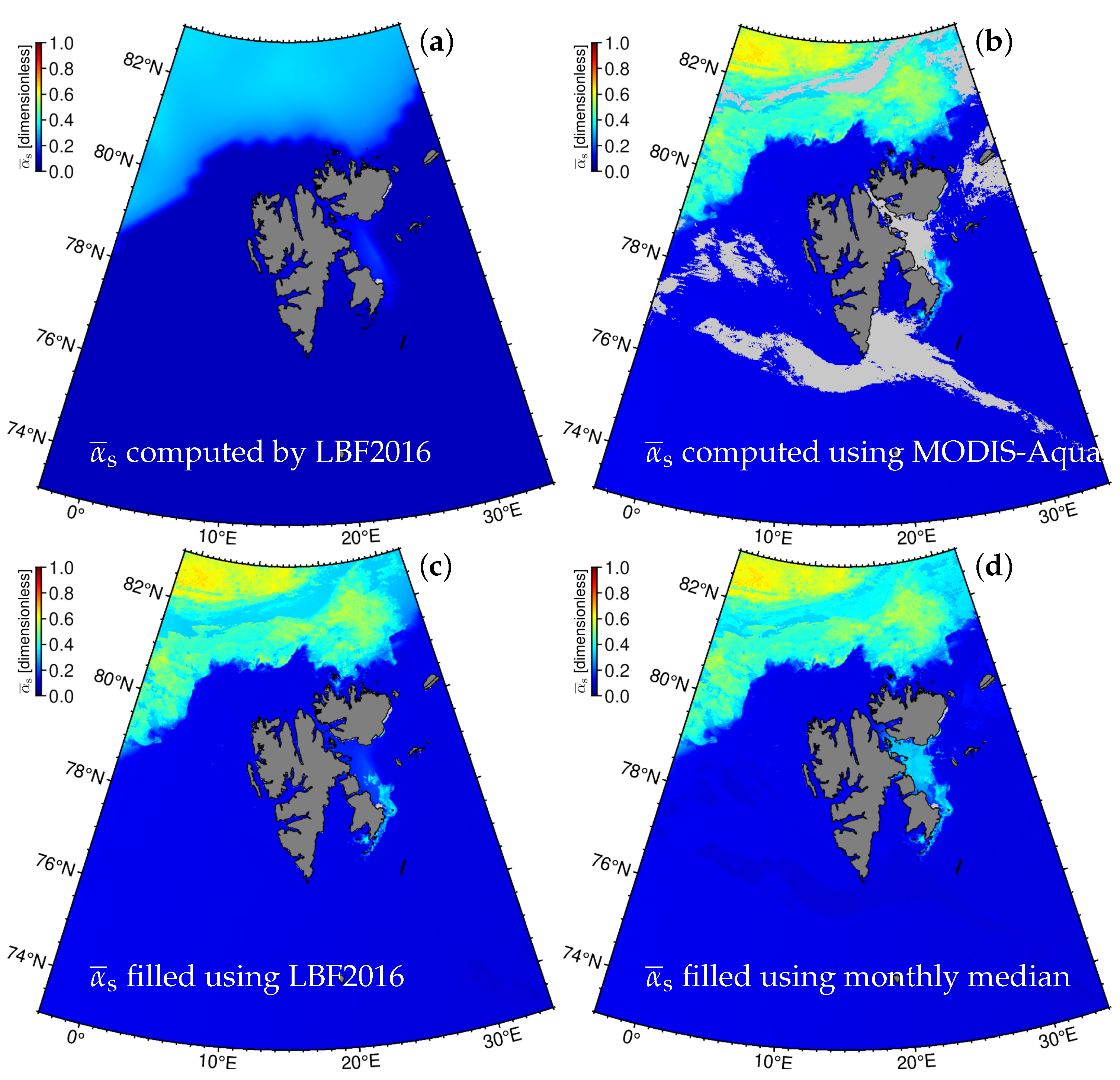
3.2. Mean Surface Albedo for PAR Bands (${\overline{\alpha }}_{\mathrm{s}}$)

The ${\overline{\alpha }}_{\mathrm{s}}$ plays a vital role in the estimation of surface PAR for bright ice-covered surfaces. Bélanger et al. [14] computed the irradiance LUT using a constant value of ${\overline{\alpha }}_{\mathrm{s}}$ pegged at 8% for all water surfaces. However, this assumption does not hold true for ice-covered water surfaces due to multiple scattering between the surface and the lower atmosphere; therefore, the LBF2016 algorithm updated the LUTs by adding the ${\overline{\alpha }}_{\mathrm{s}}$ parameter, which was estimated using

$${\overline{\alpha }}_{\mathrm{s}}={\overline{\alpha }}_{\mathrm{s}}^{\mathrm{w}}\left(1-C_{\mathrm{ice}}\right)+{\overline{\alpha }}_{\mathrm{s}}^{\mathrm{ice}}{C}_{\mathrm{ice}}$$

(4)

where the mean surface albedo for water (${\overline{\alpha }}_{\mathrm{s}}^{\mathrm{w}}$) was assumed to be 6%, and surface albedo of sea ice (${\overline{\alpha }}_{\mathrm{s}}^{\mathrm{ice}}$) was calculated as a function of day of the year for different phases of sea ice using Perovich et al. [57] in situ observations. The $C_{\mathrm{ice}}$ is available at the spatial resolution of 25 km × 25 km, which was super-sampled to 1 km × 1 km resolution to match the spatial resolution of MODIS-Aqua. However, as mentioned previously, the accuracy of passive microwave data during the melting and freezing season could be erroneous [65], as illustrated in Figure 4 (a versus b, see below). Moreover, the super-sampling of data can increase the uncertainty, especially in the coastal zone. Additionally, the rate of change of surface albedo of sea ice through the season used to calculate ${\overline{\alpha }}_{\mathrm{s}}^{\mathrm{ice}}$ also varies on a spatio-temporal scale. Therefore, in the present study, the method described in the next section was used to calculate ${\overline{\alpha }}_{\mathrm{s}}$.

3.2.1. ${\overline{\alpha }}_{\mathrm{s}}$ for Sea Ice under Clear Sky

Surface albedo at a specific wavelength (${\alpha }_{\mathrm{s}}\left(\lambda \right)$) can be estimated by the ratio of outgoing irradiance from the surface ($E_{\mathrm{s}}\left(\lambda \right)$) to the irradiance incident on the surface ($E_{\mathrm{i}}\left(\lambda \right)$) [66]. These irradiances can be estimated from satellite spectral radiance at the top-of-atmosphere (TOA) under clear sky. It should be noted that $E_{\mathrm{i}}\left(\lambda \right)$ used in this section is equal to $E_{\mathrm{d}}(\lambda ,0^{+})$. Still, different notations were used to distinguish between the approximate input irradiance used to compute ${\alpha }_{\mathrm{s}}\left(\lambda \right)$ and the more accurate output from the LUTs used in the PAR algorithm. With the help of atmospheric correction, the TOA radiance can be reduced to the bottom of atmosphere (BOA) radiance by subtracting the atmospheric path radiance ($L_{\mathrm{p}}\left(\lambda \right)$) due to atmospheric scattering. In atmospheric correction, the radiance components in the atmosphere for a linear system and the radiance components are treated as scalars; therefore, the path radiance due to scattering in the atmosphere will remain the same for the incident as well as the reflected light. In general, sea ice in the Arctic is covered with snow; therefore, by assuming sea-ice surface Lambertian [67], $E_{\mathrm{i}}\left(\lambda \right)$ and $E_{\mathrm{s}}\left(\lambda \right)$ can be estimated using $L_{\mathrm{p}}\left(\lambda \right)$, TOA radiance as measured by the sensor ($L_{\mathrm{t}}\left(\lambda \right)$), ${\theta }_0$, sensor viewing angle (${\theta }_{\mathrm{v}}$), gaseous transmittance due to atmospheric gases such as water vapour, CO${}_2$, CO, CH${}_4$ ($t_{\mathrm{g}}\left(\lambda \right)$, Gao et al. [68]) and diffuse atmospheric transmittance ($t_{\mathrm{d}}\left(\lambda \right)$, Wang [69]) for Rayleigh-aerosol atmosphere.

The TOA radiance ($L_{\mathrm{t}}$) can be expressed as [70,71,72]

$$\begin{array}{cc}\hfill L_{\mathrm{t}}\left(\lambda \right)& =\left[L_{\mathrm{R}}\left(\lambda \right)+L_{\mathrm{a}}\left(\lambda \right)+L_{\mathrm{ra}}\left(\lambda \right)+t_{\mathrm{glint}}^{\uparrow }\left(\lambda \right)L_{\mathrm{glint}}\left(\lambda \right)+t_{\mathrm{d}}^{\uparrow }\left(\lambda \right)L_{\mathrm{f}}\left(\lambda \right)+t_{\mathrm{d}}^{\uparrow }\left(\lambda \right)L_{\mathrm{w}}\left(\lambda \right)\right]\times t_{\mathrm{g}}^{\uparrow }\left(\lambda \right)\times f_{\mathrm{pol}}\left(\lambda \right)\hfill \\ \hfill & =\left[L_{\mathrm{p}}\left(\lambda \right)+t_{\mathrm{glint}}^{\uparrow }\left(\lambda \right)L_{\mathrm{glint}}\left(\lambda \right)+t_{\mathrm{d}}^{\uparrow }\left(\lambda \right)L_{\mathrm{f}}\left(\lambda \right)+t_{\mathrm{d}}^{\uparrow }\left(\lambda \right)L_{\mathrm{w}}\left(\lambda \right)\right]\times t_{\mathrm{g}}^{\uparrow }\left(\lambda \right)\times f_{\mathrm{pol}}\left(\lambda \right)\hfill \end{array}$$

(5)

where $L_{\mathrm{p}}\left(\lambda \right)$ is the atmospheric path radiance, which can be subdivided into $L_{\mathrm{R}}\left(\lambda \right)$ for Rayleigh radiance, $L_{\mathrm{a}}\left(\lambda \right)$ for aerosol radiance, and $L_{\mathrm{ra}}\left(\lambda \right)$ for the radiance due to multi-scattering. $L_{\mathrm{w}}\left(\lambda \right)$ is water-leaving radiance, $L_{\mathrm{glint}}\left(\lambda \right)$ is the radiance due to sunglint and $L_{\mathrm{f}}\left(\lambda \right)$ is caused due to whitecaps on the sea surface. $t_{\mathrm{d}}\left(\lambda \right)$ is the diffused transmittance [69] and $t_{\mathrm{glint}}\left(\lambda \right)$ is transmittance for sunglint [72]. Another loss in ${\rho }_{\mathrm{w}}\left(\lambda \right)$ will occur due to the absorption by atmospheric gases ($t_{\mathrm{g}}\left(\lambda \right)$). The arrows over $t_{\mathrm{d}}\left(\lambda \right)$, $t_{\mathrm{glint}}\left(\lambda \right)$ and $t_{\mathrm{g}}\left(\lambda \right)$ depict the path of the transmittance (↓ = sun to surface, ↑ = surface to the sensor). $f_{\mathrm{pol}}\left(\lambda \right)$ is the polarisation correction factor [73].

In the presence of sea ice, there will be no specular reflection from water, hence, $L_{\mathrm{glint}}\left(\lambda \right)\approx 0$. Furthermore, the spatially averaged $\sim 1$ km pixels of MODIS-Aqua sensor will result in negligible radiance due to whitecaps [58] making $L_{\mathrm{f}}\left(\lambda \right)\approx 0$. Therefore, Equation (5) can be written in the form of irradiance ($E\left(\lambda \right)$) using the mean earth-sun distance corrected extra-terrestrial solar irradiance for the day ($F_0\left(\lambda \right)$) and the solar-sensor geometry as

$$\pi L_{\mathrm{t}}\left(\lambda \right)cos{\theta }_{\mathrm{v}}=\left[\pi L_{\mathrm{p}}\left(\lambda \right)cos{\theta }_{\mathrm{v}}+t_{\mathrm{d}}^{\uparrow }\left(\lambda \right)E_{\mathrm{s}}\left(\lambda \right)\right]\times t_{\mathrm{g}}^{\uparrow }\left(\lambda \right)\times f_{\mathrm{pol}}\left(\lambda \right)$$

(6)

where $L_{\mathrm{p}}\left(\lambda \right)$ is the radiance due to atmospheric scattering (Rayleigh scattering, aerosol scattering and multi-scattering), ${\theta }_{\mathrm{v}}$ is the sensor zenith angle and $E_{\mathrm{s}}\left(\lambda \right)$ is the irradiance reflected from the sea-ice surface. $L_{\mathrm{p}}\left(\lambda \right)$ is computed using modified SeaDAS v7.5 to use the SSP aerosol correction algorithm [47] instead of the default option. The above equation can be re-arranged to give $E_{\mathrm{s}}\left(\lambda \right)$ as

$$E_{\mathrm{s}}\left(\lambda \right)=\pi cos{\theta }_{\mathrm{v}}\left[\frac{L_{\mathrm{t}}\left(\lambda \right)}{t_{\mathrm{g}}^{\uparrow }\left(\lambda \right)\times f_{\mathrm{pol}}\left(\lambda \right)}-L_{\mathrm{p}}\left(\lambda \right)\right]\times \frac{1}{t_{\mathrm{d}}^{\uparrow }\left(\lambda \right)}$$

(7)

Similarly, as the components of Equation (5) are scalar, the incident irradiance at the surface $E_{\mathrm{i}}\left(\lambda \right)$ can be expressed using the incident extra-terrestrial solar irradiance, $E_0\left(\lambda \right)=F_0\left(\lambda \right)cos{\theta }_0$, and as $E_{\mathrm{i}}$ is not observed by a sensor, polarisation correction is not required, hence $f_{\mathrm{pol}}\left(\lambda \right)=1$. Therefore, using Equation (7), the irradiance reaching the surface for clear sky, $E_{\mathrm{i}}^{\mathrm{clear}}\left(\lambda \right)$, can be expressed as

$$E_{\mathrm{i}}^{\mathrm{clear}}\left(\lambda \right)=\left[\frac{E_0\left(\lambda \right)}{t_{\mathrm{g}}^{\downarrow }\left(\lambda \right)}-\pi L_{\mathrm{p}}\left(\lambda \right)cos{\theta }_{\mathrm{v}}\right]\times \frac{1}{t_{\mathrm{d}}^{\downarrow }\left(\lambda \right)}$$

(8)

The bands (${\lambda }_{\mathrm{b}}$ = 469 nm, ${\lambda }_{\mathrm{g}}$ = 555 nm and ${\lambda }_{\mathrm{r}}$ = 645 nm) of MODIS-Aqua were used to calculate ${\overline{\alpha }}_{\mathrm{s}}$ to avoid band saturation in the presence of clouds and ice [74]. The spectrally weighted surface reflectance, ${\overline{\alpha }}_{\mathrm{s}}$, can be calculated as

$${\overline{\alpha }}_{\mathrm{s}}=\frac{{\displaystyle \sum _k}\frac{E_{\mathrm{s}}\left({\lambda }_k\right)}{E_{\mathrm{i}}^{\mathrm{clear}}\left({\lambda }_k\right)}\times E_0\left({\lambda }_k\right)}{{\displaystyle \sum _k}{E}_0\left({\lambda }_k\right)},k=\mathrm{b},\mathrm{g},\mathrm{r}$$

(9)

3.2.2. ${\overline{\alpha }}_{\mathrm{s}}$ for Water under Clear Sky

In the case of water pixels, radiance from the surface is very small compared to the path signal, which may increase uncertainty in the estimation of ${\overline{\alpha }}_{\mathrm{s}}$. Therefore, the ${\overline{\alpha }}_{\mathrm{s}}$ for water was calculated using mean total transmittance (${\overline{t}}_{\mathrm{t}}$) and direct transmittance (${\overline{T}}_{\mathrm{d}}$) as described by Frouin et al. [29]

$${\overline{\alpha }}_{\mathrm{s}}=\left[\frac{0.05}{1.1\times cos{{\theta }_0}^{1.4}+0.15}\right]\frac{{\overline{T}}_{\mathrm{d}}}{{\overline{t}}_{\mathrm{t}}}+0.08\times \left(1-\frac{{\overline{T}}_{\mathrm{d}}}{{\overline{t}}_{\mathrm{t}}}\right)$$

(10)

3.2.3. ${\overline{\alpha }}_{\mathrm{s}}$ under Clouds

The estimation of ${\overline{\alpha }}_{\mathrm{s}}$ under the clouds becomes difficult due to the absence of information about $E_{\mathrm{i}}\left(\lambda \right)$ and $E_{\mathrm{s}}\left(\lambda \right)$. However, as clouds are mobile and MODIS-Aqua has more than one overpass in a day over the Arctic circle, a major portion of ${\overline{\alpha }}_{\mathrm{s}}$ for cloudy pixels can be filled by the temporal mean of cloud-free data for the pixel in a day employing Equation (9) and Equation (10). However, even after multiple overpasses, it is not necessary that cloud-free ${\overline{\alpha }}_{\mathrm{s}}$ will be observed for every pixel of the scene within a day (Figure 4b). In such cases, Equation (10) can be employed to get the approximate ${\overline{\alpha }}_{\mathrm{s}}$ for water pixels under the clouds. The primary difficulty in using Equation (10) to estimate ${\overline{\alpha }}_{\mathrm{s}}$ for a pixel containing clouds is the unavailability of ${\mathsf{\tau }}_{\mathrm{a}}$ to calculate ${\overline{t}}_{\mathrm{d}}$ and ${\overline{T}}_{\mathrm{d}}$. However, scattering due to aerosols is significantly lesser than the scattering by air molecules in the Arctic region. Therefore, ${\mathsf{\tau }}_{\mathrm{a}}$ can be assumed to be zero to approximate ${\overline{\alpha }}_{\mathrm{s}}$ under the clouds.

The presence of sea ice under the clouds can increase the complexity of ${\overline{\alpha }}_{\mathrm{s}}$ retrieval. In such cases, the water surface albedo can be computed using Equation (10), assuming ${\mathsf{\tau }}_{\mathrm{a}}$ = 0 to calculate ${\overline{\alpha }}_{\mathrm{s}}$ using Equation (4). Then, the LBF2016 algorithm approach (Equation (4)) can be used to fill the gaps due to cloud cover, while accounting for the effect of sea ice on ${\overline{\alpha }}_{\mathrm{s}}$. However, lower accuracy of $C_{\mathrm{ice}}$ during the melting and freezing leads to significant uncertainties in ${\overline{\alpha }}_{\mathrm{s}}$ estimation under clouds. The uncertainty increases further in coastal waters due to super-sampling leading to substantial uncertainty in $C_{\mathrm{ice}}$ (Figure 4c). Therefore, these pixels that had clouds throughout the day were allocated with the median of the ${\overline{\alpha }}_{\mathrm{s}}$ calculated using MODIS-Aqua data for the month (Figure 4d). The approximation of ${\overline{\alpha }}_{\mathrm{s}}$ with the monthly median is essential near the coast. For example, in the east coast of Svalbard (Olgastretet) (Figure 4c), significantly low $C_{\mathrm{ice}}$ was detected by the passive microwave sensor leading to erroneous ${\overline{\alpha }}_{\mathrm{s}}$, which was corrected using the median values for the month as shown in Figure 4d. Hence, Equation (4) was used only for the pixels that have no ${\overline{\alpha }}_{\mathrm{s}}$ throughout the month due to cloud cover.

3.3. Cloud Optical Thickness (${\mathsf{\tau }}_{\mathrm{c}}$)

The presence of clouds in the atmosphere attenuates the incident light, the magnitude of this attenuation is given by cloud optical thickness (${\mathsf{\tau }}_{\mathrm{c}}$) [75]. The ${\mathsf{\tau }}_{\mathrm{c}}$ of a cloudy atmosphere is dependent on reflection, transmission and absorption [76]. However, optical remote sensing cannot see through the clouds and hence, it is difficult to compute cloud transmittance and absorption. Therefore, the following assumptions were made to compute ${\mathsf{\tau }}_{\mathrm{c}}$ from MODIS-Aqua observations (Figure 5 illustrates the different quantities defined below).

(1)

${\lambda }_{\mathrm{r}}$ (665 nm band as reference wavelength) is sensitive to the cloud optical thickness and at ${\lambda }_{\mathrm{r}}$, single scattering albedo of cloud is almost unity [77].

(2)

The absorption by clouds at ${\lambda }_{\mathrm{r}}$ is negligible [78].

(3)

The ${\mathsf{\tau }}_{\mathrm{c}}$ remains nearly spectrally constant in the visible range [79].

(4)

The transmittance of the atmosphere above the cloud is near unity.

(5)

The irradiance reflected by the surface, $E_{\mathrm{s}}$, is assumed to be transmitted to the bottom of the cloud ($E_{\mathrm{r}}\sim E_{\mathrm{s}}$).

(6)

Multiple scattering between bright sea-ice surface and bottom of the cloud is ignored.

Using these assumptions, we can compute cloud transmittance ($t_{\mathrm{c}}$) at ${\lambda }_{\mathrm{r}}$. Then $t_{\mathrm{c}}$ can be used to compute ${\mathsf{\tau }}_{\mathrm{c}}$ in the red waveband. As there is no absorption in the clouds at ${\lambda }_{\mathrm{r}}$ and single scattering albedo is near unity, the total upwelling irradiance at the TOA ($E_{\mathrm{t}}$) can be expressed as the sum of irradiance from the cloud surface ($E_{\mathrm{c}}$) and irradiance from the sea surface that has passed through the atmosphere to reach the bottom of the cloud ($E_{\mathrm{r}}$) and has transmitted through the cloud with transmittance $t_{\mathrm{c}}$. The last two assumptions listed above will have opposite impact on partition between the irradiance reflected back directly by the cloud, $E_{\mathrm{c}}$, and the irradiance coming from the surface that was transmitted through the clouds ($t_{\mathrm{c}}{E}_{\mathrm{r}}$) (Figure 5). Assumption 5 will overestimate $E_{\mathrm{r}}$ (or $E_{\mathrm{s}}$), while assumption 6 will underestimate the surface irradiance under clouds, $E_{\mathrm{i}}^{\mathrm{cloud}}$, and therefore $E_{\mathrm{s}}$. All these quantities are a function of $\lambda$ and were calculated at ${\lambda }_{\mathrm{r}}$, but it is not shown in the equation for brevity.

$$E_{\mathrm{t}}=E_{\mathrm{c}}+t_{\mathrm{c}}{E}_{\mathrm{r}}$$

(11)

Moreover, $E_{\mathrm{c}}$ can be expressed as the difference between the total incident irradiance over the cloud ($E_0$) and the irradiance transmitted through the cloud ($t_{\mathrm{c}}{E}_0$). In other words, the incident irradiance that is not transmitted through the clouds is assumed to be reflected [77]. Therefore, Equation (11) can be rewritten as

$$\begin{array}{cc}\hfill E_{\mathrm{t}}& =\left(1-t_{\mathrm{c}}\right)E_0+t_{\mathrm{c}}{E}_{\mathrm{r}}\hfill \\ \hfill & =\left(E_0-t_{\mathrm{c}}{E}_0\right)+t_{\mathrm{c}}{E}_{\mathrm{r}}\hfill \end{array}$$

(12)

Here $E_{\mathrm{t}}$ and $E_0$ values are available, but $E_{\mathrm{r}}$ is missing. To retrieve this quantity, we first computed the surface irradiance assuming there is no cloud using Equation (8) (i.e., $E_{\mathrm{i}}^{\mathrm{clear}}$). However, in the presence of cloud, $t_{\mathrm{c}}{E}_0$ will interact with the atmosphere. Hence, the irradiance incident on the surface in the presence of cloud ($E_{\mathrm{i}}^{\mathrm{cloud}}$) could be approximated as $t_{\mathrm{c}}{E}_{\mathrm{i}}^{\mathrm{clear}}$. If the surface albedo, ${\alpha }_{\mathrm{s}}$, below the cloud is known, then the irradiance reflected by the surface can be assessed. Therefore, $E_{\mathrm{s}}$ can be expressed as

$$\begin{array}{cc}\hfill E_{\mathrm{s}}& ={\alpha }_{\mathrm{s}}{E}_{\mathrm{i}}^{\mathrm{cloud}}\hfill \\ \hfill & ={\alpha }_{\mathrm{s}}{t}_{\mathrm{c}}{E}_{\mathrm{i}}^{\mathrm{clear}}\hfill \end{array}$$

(13)

Here the ${\alpha }_{\mathrm{s}}$ is computed at ${\lambda }_{\mathrm{r}}$ using the method described in Section 3.2.3, which is based in a clear sky estimation of ${\alpha }_{\mathrm{s}}$ and on a gap-filling approaches when persistent cloud cover is present (see above for details). However, due to computational constraints, for computation of $t_{\mathrm{c}}$, the ${\alpha }_{\mathrm{s}}$ is estimated using passive microwaves as in LBF2016.

$E_{\mathrm{s}}$ when it passes through the atmosphere to reach the bottom of the cloud ($E_{\mathrm{r}}$), it encounters diffusion and scattering in the atmosphere. However, it is difficult to quantify these effects using optical data under the clouds. Furthermore, these effects will result in a loss (due to diffusion) as well as a gain (due to atmospheric scattering, see Equation (5)) in the signal. Besides, the strength of $E_{\mathrm{r}}$ would be significantly low as compared to $(1-t_{\mathrm{c}})E_0$. Therefore, for simplicity, we have not considered the atmospheric effects and multi-scattering between bright sea-ice surface and clouds while calculating $E_{\mathrm{r}}$, making $E_{\mathrm{r}}$ equal to $E_{\mathrm{s}}$. Besides, as stated in the assumptions, the underestimated $E_{\mathrm{i}}^{\mathrm{cloud}}$, as a consequence of ignoring the multi-scattering between the bright sea-ice and cloud would compensate for the overestimation in the calculation of $E_{\mathrm{r}}$. Moreover, including multi-scattering in the atmosphere below the cloud could help reduce the uncertainty in the computed $E_{\mathrm{r}}$ [80].

Substituting Equation (13) in Equation (12) and using the quadratic formula $t_{\mathrm{c}}$ can be expressed as

$$t_{\mathrm{c}}=\frac{E_0-\sqrt{E_0^2-4{\alpha }_{\mathrm{s}}{E}_{\mathrm{i}}\left(E_0-E_{\mathrm{t}}\right)}}{2{\alpha }_{\mathrm{s}}{E}_{\mathrm{i}}}$$

(14)

Pandey et al. [81] implemented a semi-analytical algorithm to relate cloud transmittance $t_{\mathrm{c}}$ to ${\mathsf{\tau }}_{\mathrm{c}}$.

$${\mathsf{\tau }}_{\mathrm{c}}=\frac{1}{0.75}\times \left(\frac{1}{t_{\mathrm{c}}}-\gamma \right)\times \left(\frac{1}{1-g}\right)$$

(15)

Here, g is the cloud asymmetry factor with a value of 0.85, and $\gamma$ is 1.07.

An example of ${\mathsf{\tau }}_{\mathrm{c}}$ computed using $t_{\mathrm{c}}$ from MODIS-Aqua data is presented in Figure 6a. The use of $t_{\mathrm{c}}$ to compute ${\mathsf{\tau }}_{\mathrm{c}}$ works effectively for thick clouds over sea ice and open water. However, for thin clouds over sea ice (e.g., the clouds over sea ice in north of Svalbard, see Figure 3), ${\mathsf{\tau }}_{\mathrm{c}}$ is significantly overestimated as it becomes difficult to distinguish $E_{\mathrm{c}}$ and $E_{\mathrm{r}}$ at ${\lambda }_{\mathrm{r}}$. The higher value of $E_{\mathrm{r}}$ is interpreted as $E_{\mathrm{c}}$ resulting in a lower values of $t_{\mathrm{c}}$ giving a significantly high ${\mathsf{\tau }}_{\mathrm{c}}$.

3.4. Calculation of PAR

3.4.1. PAR at Sea Surface

To calculate daily PAR at the sea surface, for each day, the period from sunrise ($T_{\mathrm{rise}}$) to sunset ($T_{\mathrm{set}}$) was divided into ten equal parts, and ${\theta }_0$ was calculated at each time step (T). The ${\theta }_0$ values were provided as input to the LUTs, while keeping ${\mathsf{\tau }}_{\mathrm{oz}}$, ${\mathsf{\tau }}_{\mathrm{c}}$ and ${\overline{\alpha }}_{\mathrm{s}}$ constant, to calculate $E_{\mathrm{d}}(\lambda ,0^{+},T)$ and $E_{\mathrm{d}}(\lambda ,0^{-},T)$. These $E_{\mathrm{d}}$ at different time steps were then integrated over PAR wavelengths to give instantaneous PAR for that time of the day. These instantaneous PAR values were then integrated through the day to yield daily PAR using data from one overpass. The daily PAR values from different overpasses were averaged to get the daily integral PAR value for the day as shown in Figure 6b for above water PAR, and Figure 7 for PAR just below the sea surface using Equation (16).

$${\displaystyle \mathrm{PAR}\left(s\right)=\frac{1}{M}\sum _{m=1}^M{\int }_{T=T_{\mathrm{rise}}}^{T_{\mathrm{set}}}{\int }_{\lambda =400\mathrm{nm}}^{700\mathrm{nm}}{E}_{\mathrm{d},m}(\lambda ,s,T)d\lambda dT}$$

(16)

Here, s can be $0^{+}$ for PAR just above the sea surface and $0^{-}$ for PAR just below the sea surface (for open water), and M is the number of satellite overpasses in a day over the region.

3.4.2. PAR Penetrating the Sea Surface in the Presence of Ice

The presence of sea ice in the Arctic region is another critical factor affecting PAR entering the water column. The magnitude and shape of the spectra transmitting through ice depend upon thickness, surface conditions and physical composition [83]. Therefore, it is challenging to estimate light penetration through the sea ice from space-borne sensors, and assumptions are needed. According to Maykut and Grenfell [84], the maximum transmittance through a 185 cm thick ice was <20% (for green bands) for all surface conditions. On the ond hand, sea ice is often covered with snow, which can be turbid in the coastal region, further reducing the light penetration through the sea ice and changing the surface albedo. On the other hand, an optically thick layer of ice algae at the bottom of sea ice can attenuate (scattering from sea ice matrix and absorption) most of the PAR transmitted through the snow-ice, reducing the light transmission to the water column close to zero, e.g., [26]. Therefore, if it is assumed that the light is scattered from the surface only and a fraction of the remaining light is lost within the ice pack due to absorption, hereafter referred to as $\eta$, then the PAR($0^{-}$) just below the sea ice can be estimated by adding the $\eta$ component to the expression described by Laliberté [82] as

$$\mathrm{PAR}\left(0^{-}\right)=\left(1-\eta \right)\left(1-{\overline{\alpha }}_{\mathrm{s}}\right)\mathrm{PAR}\left(0^{+}\right)$$

(17)

Note that $\eta$ is not equal to the absorptance (i.e., the ratio of the absorbed to the incident radiant power) of the ice/snow cover, which is largely unknown for Arctic sea ice. Therefore, the summation of $\eta$, transmittance and reflectance will not be unity. $\eta$ varies through the season based on the thickness of sea ice and the presence of absorbing material in the snow and ice (ice-algae, mineral, organic matter, etc.) and mostly remains close to 0.8 during the winters [82], such that 80% of the PAR that penetrates the ice/snow cover (i.e., $\left(1-{\overline{\alpha }}_{\mathrm{s}}\right)\mathrm{PAR}\left(0^{+}\right)$ ) is lost due to absorption by snow, ice, impurities or ice algae. $\eta$ decreases during the summer as the sea-ice thickness decreases, the snow cover diminishes and ice-algae are flushed out [85]; therefore, it is not possible to quantify the change in $\eta$ from space-borne observations. Consequently, a range of PAR(0${}^{-}$) bound with $\eta =0.8$ (high loss of light in the sea-ice matrix yielding lower limit for PAR(0${}^{-}$)) and $\eta =0$ (no sea-ice cover, hence no loss of light due to sea ice; upper limit) is calculated. The upper and lower limit of the under-water light penetration is shown in Figure 7a and Figure 7b, respectively.

3.4.3. PAR at Seafloor

PAR at the seafloor (PAR($z_{\mathrm{b}}$)), where $z_{\mathrm{b}}$ denotes the bottom depth (Figure 8a), can be calculated by integrating downwelling irradiance at the seafloor ($E_{\mathrm{d}}(\lambda ,z_{\mathrm{b}},T)$). The depth limit chosen for this study was set at 100 m depth. The choice of depth limit is based on the finding of Krause-Jensen et al. [86], who reported the presence of kelp at 61 m depth offshore on the east coast of Greenland. Moreover, some Arctic kelp species can have a compensating irradiance in the order of 0.1–0.3 mol m${}^{-2}$ day${}^{-1}$ [87,88]. $E_{\mathrm{d}}(\lambda ,z_{\mathrm{b}},T)$ can be computed from $E_{\mathrm{d}}(\lambda ,0^{-},T)$ and depth-averaged downwelling diffused attenuation coefficient (${\overline{K}}_{\mathrm{d}}\left(\lambda \right)$) using the Beer-Lambert law

$${\displaystyle \mathrm{PAR}\left(z_{\mathrm{b}}\right)=\frac{1}{M}\sum _{m=1}^M{\int }_{T=T_{\mathrm{rise}}}^{T_{\mathrm{set}}}{\int }_{\lambda =400\mathrm{nm}}^{700\mathrm{nm}}{E}_{\mathrm{d},m}(\lambda ,0^{-},T)e^{-z_{\mathrm{b}}{\overline{K}}_{\mathrm{d},m}\left(\lambda \right)}d\lambda dT=\frac{1}{M}\sum _{m=1}^M\mathrm{PAR}{\left(0^{-}\right)}_m{e}^{-z_{\mathrm{b}}{K}_{\mathrm{d},m}^{\mathrm{PAR}}}}$$

(18)

${\overline{K}}_{\mathrm{d}}\left(\lambda \right)$ or $K_{\mathrm{d}}^{\mathrm{PAR}}$ (shown in Figure 8b) can be estimated with a significant accuracy (uncertainty ∼ 7–26%) using the absorption and back-scattering in the water column [41,42]. However, varying optically active constituent (OAC) concentration (such as coloured dissolved organic matter (CDOM), SPM and $C_{\mathrm{Chl}-a}$) under the sea ice can change $K_{\mathrm{d}}^{\mathrm{PAR}}$, thereby altering the underwater light field [89,90]. Hence, approximating $K_{\mathrm{d}}^{\mathrm{PAR}}$ below the sea ice can be erroneous, and the uncertainty in retrieving absorption coefficient through satellite-borne sensors can reach 40% in the AO [91]. Autonomous systems can be used to retrieve $K_{\mathrm{d}}^{\mathrm{PAR}}$ below sea ice, but the implementation of these systems is still at a nascent stage [15]. Therefore, $K_{\mathrm{d}}^{\mathrm{PAR}}$ for the cloudy and sea-ice covered pixels is approximated with the monthly median of $K_{\mathrm{d}}^{\mathrm{PAR}}$ (Figure 8c). This approximate value of $K_{\mathrm{d}}^{\mathrm{PAR}}$ can be used to estimate PAR($z_{\mathrm{b}}$) for most of the coastal region, as shown in Figure 8d. However, when $K_{\mathrm{d}}^{\mathrm{PAR}}$ is not available for some pixels due to sea-ice/cloud cover or lack of incident light for the whole month, PAR($z_{\mathrm{b}}$) is not calculated. For example, due to sea-ice cover over the northern part of Svalbard and east coast of Barentsøya and Edgeøya (Figure 8b,c) for the whole month of July 2020, median $K_{\mathrm{d}}^{\mathrm{PAR}}$ was absent and hence, PAR($z_{\mathrm{b}}$) was not calculated. As a result, our method will underestimate PAR reaching the seafloor at the beginning of the spring and summer season when ice cover is still present.

3.5. Validation of Calculated PAR with In Situ Data

The statistical measures (such as the slope of regression ($\mathfrak{m}$) and correlation coefficient (r)) are based on the assumption that uncertainty follows Gaussian distribution [92]. As the distribution of uncertainty in the present study was almost Gaussian (Figure 9b), $\mathfrak{m}$, and r were used to evaluate the performance of the PAR algorithm. However, these metrics alone cannot address the non-linearity and systematic difference in the results. Therefore, it is necessary to calculate other statistics such as bias, median percentage difference (MPD), the median of the ratio of calculated and in situ PAR (mR${}_{\mathrm{si}}$) and semi-interquartile range (SIQR) [92,93,94,95]. The expressions to calculate these metrics using the satellite-derived PAR (PAR${}_{\mathrm{Sat}}$) and in situ PAR (PAR${}_{insitu}$) for N observations are shown in the following equations. PAR${}_{insitu}$ and PAR${}_{\mathrm{Sat}}$ are referred to as X and Y, respectively, in these equations for brevity.

$$\mathfrak{m}=\frac{N{\displaystyle \sum _{i=1}^N}{X}_i{Y}_i-{\displaystyle \sum _{i=1}^N}{X}_i{\displaystyle \sum _{i=1}^N}{Y}_i}{N{\displaystyle \sum _{i=1}^N}{\left(X_i\right)}^2-{\left({\displaystyle \sum _{i=1}^N}{X}_i\right)}^2}$$

(19)

$$r=\frac{{\displaystyle \sum _{i=1}^N}\left(X_i-\overline{X}\right)\left(Y_i-\overline{Y}\right)}{\sqrt{{\displaystyle \sum _{i=1}^N}{\left(X_i-\overline{X}\right)}^2}\sqrt{{\displaystyle \sum _{i=1}^N}{\left(Y_i-\overline{Y}\right)}^2}}$$

(20)

here, $\overline{X}$ and $\overline{Y}$ are mean PAR${}_{insitu}$ and mean PAR${}_{\mathrm{Sat}}$, respectively.

$$\mathrm{Bias}=\frac{1}{N}\times \sum _{i=1}^N\left(Y_i-X_i\right)$$

(21)

$$\mathrm{MPD}=\mathrm{median}\left\{\frac{\left|Y-X\right|}{X}\times 100\right\}$$

(22)

$${\mathrm{mR}}_{\mathrm{si}}=\mathrm{median}\left\{\frac{Y}{X}\right\}$$

(23)

$$\mathrm{SIQR}=\frac{Q_3-Q_1}{2}$$

(24)

here, $Q_1$ and $Q_3$ are ${25}^{\mathrm{th}}$ and ${75}^{\mathrm{th}}$ percentiles of $\frac{Y}{X}$, respectively.

4. Results and Discussion

The use of MODIS-Aqua data to derive the input parameters for the PAR LUTs has reduced the algorithm’s dependency on other sources, making it robust and increasing its applicability. This is suggested to be a significant improvement relative to the previous LBF2016 method evaluated in the Arctic and by Somayajula et al. [31] in the Mediterranean Sea. However, these changes make it necessary to check the performance of the algorithm and validate the output PAR. The daily integral PAR($0^{+}$) and PAR($z_{\mathrm{b}}$) can be obtained from the stations/moorings deployed at the surface and seafloor (or at a specific depth, z). However, it is not easy to install PAR sensor just below the water surface and record in situ values for daily PAR($0^{-}$). Therefore, only daily PAR($0^{+}$) and PAR($z_{\mathrm{b}}$) were validated using the in situ data obtained in coastal waters (see Table 1). Moreover, PAR($z_{\mathrm{b}}$) is a function of PAR($0^{-}$) and $K_{\mathrm{d}}^{\mathrm{PAR}}$ (Equation (18)); therefore, PAR($z_{\mathrm{b}}$) can be used as a proxy to validate the efficacy of PAR($0^{-}$) and $K_{\mathrm{d}}^{\mathrm{PAR}}$ (

Table 2. Performance parameters calculated to validate the daily PAR derived from the satellite data.

Position (Depth)	Station/Mooring	mR${}_{\mathbf{si}}$ (±SIQR)	MPD (%)	Bias	$\mathfrak{m}$	r	N
Sea surface ($0^{+}$ m)	C33-JB	1.03 (±0.18)	19.29	0.87	0.83	0.76	132
	V31-JB
	Endeavor
	MPI	1.14 (±0.21)	24.47	3.81	1.10	0.94	1190
	ISA	0.63 (±0.16)	37.36	−9.47	1.10	0.90	378
Seafloor (6.1 m)	DS11	1.48 (±1.03)	76.71	0.54	0.71	0.74	381
Seafloor (4.4 m)	E1
Seafloor (4.3 m)	E2
Seafloor (5.5 m)	L1
Seafloor (6.0 m)	W1
Seafloor (6.2 m)	W2
Seafloor (6.6 m)	W3
Subsurface (1.2 m)	IAF

Note: The total depth of IAF station is 13 m. mR_si is the median of PAR_Sat/PAR_insitu, $\mathfrak{m}$ is the regression slope, r is the Pearson’s coefficient of correlation and N is the number of observations. Unit of SIQR and bias is mol m⁻² day⁻¹. $\mathfrak{m}$ and r for MPI, ISA and PAR at the seafloor/subsurface (PAR(z_b)) were calculated using log-transformed data as recommended by Bailey and Werdell [93].

). The uncertainty of the PAR model was also computed exclusively for days when the stations were covered with sea ice (

Table 3. Performance of the developed PAR algorithm in the presence of sea-ice cover.

Measurement Depth (m)	Station/Mooring	mR${}_{\mathbf{si}}$ (±SIQR)	MPD (%)	Bias	$\mathfrak{m}$	r	${\mathit{N}}_{\mathbf{cloud}}$	${\mathit{N}}_{\mathbf{total}}$
$0^{+}$	MPI	1.15 (±0.20)	24.27	3.58	1.08	0.94	373	892
	ISA	0.60 (±0.17)	40.31	−7.92	1.04	0.92	72	115
6.1	DS11	0.79 (±1.03)	61.07	0.12	0.61	0.48	11	18
4.4	E1
4.3	E2
6.2	W2
1.2	IAF

Note: Average value of η = 0.4 is used to calculate PAR(z_b) below sea ice. N_total is the total number of data points with sea-ice cover and N_cloud is the number of data points which have cloud cover along with sea-ice.

) to check the performance and consistence of PAR computed using present study in the presence of sea ice.

4.1. Accuracy of PAR($0^{+}$) Derived from Satellite

The computed daily integral PAR($0^{+}$) during summer (July and August) was validated using the data from three stations (C33-JB and V31-JB in James Bay and Endeavor in Alaska) with 132 daily integral PAR($0^{+}$) (Table 2). The scatter-plot of the data from these stations for the present study (Figure 9a) was plotted to visualise the relationship between in situ and computed PAR($0^{+}$) values and error statistics were calculated. Figure 9a indicates a slight overestimation (mR${}_{\mathrm{si}}$ = 1.03 and bias = 0.87 mol m${}^{-2}$ day${}^{-1}$) for the PAR($0^{+}$) computed using our method. At the same time, a moderately low spread (SIQR = ±0.18 mol m${}^{-2}$ day${}^{-1}$) of the ratio of satellite-derived PAR and in situ PAR was observed. The near-unity mR${}_{\mathrm{si}}$ and low bias signifies a good agreement between the in situ and computed daily integrated PAR($0^{+}$) for these stations. The MPD ignores the outliers in the relative difference; therefore, MPD = 19.29% suggests that the relative difference for most data points lies around 19.29% (here, 67 out of 132 data points have relative uncertainty <20%) for the three stations. The in situ daily integral PAR($0^{+}$) for these stations varied from 10.26 mol m${}^{-2}$ day${}^{-1}$ to 55.13 mol m${}^{-2}$ day${}^{-1}$. The $\mathfrak{m}$ and r values are relatively close to unity and are similar to the values reported by Somayajula et al. [31] for the LBF2016, which concludes that the effect of change in the input parameters to the LUTs is minimal.

The time-series plot (Figure 10) for these three stations depict a close correlation between the PAR($0^{+}$) values observed by the in situ sensors and the values computed using the OBPG algorithm and the present study (denoted by PS) from MODIS-Aqua data. The standard NASA PAR product (OBPG algorithm [29]) used in this figure was downloaded from OBDAAC at 9 km spatial resolution. Note that OBPG algorithm is not applicable in icy waters, hence, no data is available for the Endeavor site (Figure 10a). The daily PAR($0^{+}$) values from OBPG algorithm for the James Bay stations follow the trend of in situ daily PAR($0^{+}$) values, but it consistently overestimated the in situ PAR($0^{+}$) values. Besides, the daily PAR($0^{+}$) values computed using the present study capture the daily in situ variability in PAR($0^{+}$) more closely, confirming the validity of the assumptions made to retrieve the cloud optical thickness.

To evaluate the performance of the PAR algorithm in the Arctic coastal waters throughout the year, the data from two stations, MPI in Stefansson Sound (coast of Alaska) and ISA in Isfjorden (Svalbard), were used. MPI and ISA are located in the coastal region at 70.35°N and 78.22°N latitudes, respectively, (see Table 1 and Figure 2 for more details). Therefore, the data from these stations can provide good insight into the performance of the PAR algorithm year round. However, in situ PAR recorded for the days when ${\theta }_0>{85}^{\circ }$ at noon or days when the sensor recorded negative instantaneous PAR are discarded.

The overestimation by the PAR algorithm at MPI (Figure 11a) was quantified by deviation of mR${}_{\mathrm{si}}$ from the ideal value of 1 to 1.14 and bias of 3.81 mol m${}^{-2}$ day${}^{-1}$ (Table 2). The relatively higher value of bias can be attributed the deviation of in situ PAR sensor at sub-zero temperatures. The higher SIQR compared to the previous case indicates a larger spread in the PAR${}_{\mathrm{Sat}}$ and PAR${}_{insitu}$ ratio, which was expected as the range of in situ PAR for MPI varies from 0.51 mol m${}^{-2}$ day${}^{-1}$ in winter to 50.14 mol m${}^{-2}$ day${}^{-1}$ in summer (two order of magnitude). For this range of data, the MPD is 24.47% with near-unity $\mathfrak{m}$ and r (Table 2). The near unity $\mathfrak{m}$ and r suggest the algorithm works relatively well regardless of the high SIQR and can be applied to the Arctic waters throughout the year consistently. Furthermore, 1190 daily integrated PAR($0^{+}$) from 2007 to 2018 were used to calculate these performance statistics, demonstrating the robustness of the PAR algorithm.

Additionally, the performance of the algorithm was tested with 381 daily integrated PAR($0^{+}$) data from the northernmost station (ISA) in this study. The performance metrics for this station indicate a notable underestimation (Table 2), especially under low sun elevation (${\theta }_0>{70}^{\circ }$) (Figure 11b). It has resulted in a significantly low mR${}_{\mathrm{si}}$ and bias; the MPD have also increased to 37.36% when compared to the uncertainty estimated for MPI. The higher bias in the PAR retrieval could be a result of higher uncertainty in the in situ measurement (i.e., the HOBO versus LICOR sensors) and the increased uncertainty in retrieval of input parameters for the PAR model using remote sensing over land.

Moreover, at ISA the data is observed under cloud cover for 277 days out of the total 378 days resulting in higher uncertainty in ${\overline{\alpha }}_{\mathrm{s}}$ approximation and the retrieval of ${\mathsf{\tau }}_{\mathrm{c}}$ over sea ice. Furthermore, the algorithm tends to underestimate the PAR with ${\theta }_0$ beyond ${70}^{\circ }$ because the SBDART algorithm, used to compute the LUTs, assumes a plane-parallel atmosphere to solve the radiative transfer Equation [31,96]. Therefore, the PAR values estimated by the present study for ${\theta }_0$ beyond 70° were underestimated by $\sim 30\%$.

However, the higher uncertainties are encountered only during winter when coastal water of the AO are usually covered with sea ice. The lower PAR($0^{+}$) during winter (Figure 11) in the presence of sea ice with significantly high ${\overline{\alpha }}_{\mathrm{s}}$ and $\eta$ will result in very low PAR reaching the seafloor (PAR($z_{\mathrm{b}}$) < 0.17 mol m${}^{-2}$ day${}^{-1}$). In general, this low magnitude of PAR would not be sufficient to sustain the positive growth rates of primary producers [87,88]. Besides, the performance of the present study at ISA was consistent with similar uncertainty when the parameters are calculated exclusively for days when sea-ice cover was present at the station (Table 3).

4.2. Uncertainty in Satellite Estimation of PAR($z_{\mathrm{b}}$)

PAR($z_{\mathrm{b}}$) is a function of PAR($0^{-}$) and $K_{\mathrm{d}}^{\mathrm{PAR}}$ (Equation (18)); consequently, the uncertainty in the retrieval of these parameters will propagate to the uncertainty of PAR($z_{\mathrm{b}}$) computation. Therefore, the validation of PAR($z_{\mathrm{b}}$) will help ascertain the performance of the LUTs to compute PAR($0^{-}$) and the method to calculate $K_{\mathrm{d}}^{\mathrm{PAR}}$. The 435 daily in situ PAR($z_{\mathrm{b}}$) values ranges from a minimum of 1.8 × 10⁻⁴ mol m${}^{-2}$ day${}^{-1}$ to the maximum of 39.00 mol m${}^{-2}$ day${}^{-1}$. However, the accuracy of the PAR sensor at such low values cannot be ascertained; therefore, only 381 daily in situ PAR($z_{\mathrm{b}}$) values greater than 0.01 mol m${}^{-2}$ day${}^{-1}$ are used for validating the results of the present study. These in situ daily PAR($z_{\mathrm{b}}$) values were recorded by seven sensors on moorings attached to the bottom in the coastal waters of Stefansson Sound in the Beaufort Sea off-Alaskan coast and one mooring (IAF) in the catchment area of Adventfjorden in Isfjorden. For the mooring at IAF, PAR is computed at 1.2 m depth (depth at which the sensor is deployed) instead of the bottom, which was 13 m deep.

The daily PAR($z_{\mathrm{b}}$) values include 137 observations under clouds/sea ice, and hence, approximate $K_{\mathrm{d}}^{\mathrm{PAR}}$ was used to estimate satellite-derived daily PAR($z_{\mathrm{b}}$) (see Section 3.4.3). The statistics for PAR($z_{\mathrm{b}}$) presented in Table 2 are computed using $\eta =0$, as the moorings recording PAR($z_{\mathrm{b}}$) were deployed only in summer when $\eta$ approaches zero due to formation of melt ponds and leads. The low bias with r and $\mathfrak{m}$ approaching unity illustrates the good agreement between the in situ and satellite-derived PAR($z_{\mathrm{b}}$) (Table 2). Moreover, around 42% of the in situ data points were observed under sea ice (triangles in Figure 12a) or clouds (squares in Figure 12b).

The broad range of in situ PAR($z_{\mathrm{b}}$) (i.e., three to four orders of magnitude) resulted in a higher SIQR of 1.03 mol m${}^{-2}$ day${}^{-1}$ and a significant deviation of mR${}_{\mathrm{si}}$ from unity, signifying overestimation. The overestimation of PAR($z_{\mathrm{b}}$) was expected as satellite-derived $K_{\mathrm{d}}^{\mathrm{PAR}}$ cannot account for the attenuation in the benthic nepheloid layers resulting in underestimation of effective $K_{\mathrm{d}}^{\mathrm{PAR}}$ for the water column [36]. Furthermore, in general, the higher MPD values can be attributed to the fact that for very small PAR($z_{\mathrm{b}}$) (on the order of ${10}^{-2}$ mol m${}^{-2}$ day${}^{-1}$), a minor deviation in the computed values will result in a higher relative difference. Another source of higher MPD in PAR($z_{\mathrm{b}}$) could be the uncertainty in in situ data due to the precision of the PAR sensors while recording near-zero values of PAR. Despite higher MPD, the computed PAR($z_{\mathrm{b}}$) demonstrates a firm agreement with the in situ daily integrated PAR($z_{\mathrm{b}}$) from all eight moorings (Figure 12), establishing the robustness of the satellite-derived daily integral PAR($z_{\mathrm{b}}$). Consequently, the estimation of PAR($z_{\mathrm{b}}$) under sea-ice and cloud cover remain consistent with slight deviation in the uncertainty metrics (Table 3) when compared with the uncertainty estimates reported in Table 2.

4.3. Comparison with Existing Algorithm

Gattuso et al. [34] used the NASA standard OBPG algorithm to calculate PAR at the surface and used Morel [35] to estimate $K_{\mathrm{d}}^{\mathrm{PAR}}$, which uses $C_{\mathrm{Chl}-a}$ as a proxy. In a more recent study, Gattuso et al. [36] improved the estimation of $K_{\mathrm{d}}^{\mathrm{PAR}}$ using Morel et al. [97], though it was still dependent on $C_{\mathrm{Chl}-a}$ only. In addition, while the OBPG algorithm can retrieve PAR with high accuracy [31], it tends to overestimate PAR in JB, and it is limited to ice-free waters defined by $C_{\mathrm{ice}}<0.1$, limiting its applicability in icy Arctic waters (as shown in Figure 10) [25,32].

The rising temperature in the AO has resulted in the thawing of the ice on land and sea ice retreat resulting in increased terrestrial input and its re-suspension in the littoral zone [19]. These processes significantly increase the CDOM, SPM and $C_{\mathrm{Chl}-a}$ in the coastal AO, affecting the light reaching the seafloor [19,98,99]. Therefore, $K_{\mathrm{d}}^{\mathrm{PAR}}$, used by Gattuso et al. [36], underestimates the absorption and scattering in the water column nearshore due to increased optical complexity by the OACs, leading to higher PAR($z_{\mathrm{b}}$) estimation near the coastline (Figure 13a). On the contrary, the PAR($z_{\mathrm{b}}$) values estimated in the present study show significantly lower values as compared to Gattuso et al. [36] in the near-shore waters (Figure 13b). The difference between the PAR($z_{\mathrm{b}}$) values estimated by the two algorithms is more dominant in the shallower regions of the coastal AO in the eastern hemisphere. For example, in the near-shore waters of the Kara Sea, Gattuso et al. [36] computed PAR($z_{\mathrm{b}}$) values around 10 mol m${}^{-2}$ day${}^{-1}$ (Figure 13c) while PAR($z_{\mathrm{b}}$) values estimated by the present study vary around 0.1–1 mol m${}^{-2}$ day${}^{-1}$ (Figure 13d). The lower value of PAR($z_{\mathrm{b}}$) estimated by the present study can be attributed to the higher riverine inputs leading to a higher concentration of OACs, especially SPM, resulting in a significant attenuation of light [100,101].

The higher values of PAR($z_{\mathrm{b}}$) estimated by Gattuso et al. [36] can also be attributed to the usage of PAR($0^{+}$) to estimate PAR($z_{\mathrm{b}}$). Frouin et al. [29] calculates PAR($0^{+}$), which is translated to the seafloor using $K_{\mathrm{d}}^{\mathrm{PAR}}$, instead of PAR($0^{-}$). For higher ${\theta }_0$, the surface reflectivity increases exponentially [102]; hence, PAR($0^{-}$) becomes significantly less than PAR($0^{+}$). Therefore, using PAR($0^{+}$) to calculate PAR($z_{\mathrm{b}}$) can lead to significant over-estimation in the polar regions.

Furthermore, it is essential to approximate ${\overline{K}}_{\mathrm{d}}\left(\lambda \right)$ or $K_{\mathrm{d}}^{\mathrm{PAR}}$ for cloud/ice pixels, for which $K_{\mathrm{d}}$ cannot be calculated from satellite data. Ignoring the cloud/ice pixels due to the absence of $K_{\mathrm{d}}$ while estimating PAR($z_{\mathrm{b}}$) can lead to significant overestimation due to the exclusion of lower PAR($z_{\mathrm{b}}$) values under sea ice and clouds.

4.4. Trends of PAR($z_{\mathrm{b}}$) in the Coastal AO: A Brief Overview

A detailed analysis of the trends in PAR reaching the seafloor in the AO is beyond the scope of this study, but here we present a brief overview of the application of the method to assess the pan-Arctic trend as a case study. The magnitude of PAR reaching the seafloor in the coastal AO is mainly affected by the atmospheric turbidity (primarily due to clouds/fog), sea-ice cover and its snow cover and ice-algal content, and water transparency controlled by CDOM concentration and/or turbidity. The effect of these factors on PAR($z_{\mathrm{b}}$) can be accounted for by using PAR($0^{-}$) computed in the presence of clouds and sea ice, and $K_{\mathrm{d}}^{\mathrm{PAR}}$, which quantifies the attenuation of the PAR within the water column. The computed daily PAR($z_{\mathrm{b}}$) remained very low throughout the year for a major part of the coastal zone (Figure 13). Hence, the annual mean of daily PAR($z_{\mathrm{b}}$) for the pan-Arctic region would get dominated by these near-zero values resulting in very low average coastal PAR($z_{\mathrm{b}}$).

Therefore, a threshold of PAR($z_{\mathrm{b}}$) can be utilised to identify the pixels which should be included to compute the daily average PAR($z_{\mathrm{b}}$) for the pan-Arctic region. Borum et al. [87] reported that a minimum compensation radiance of 0.17 mol m${}^{-2}$ day${}^{-1}$ is required to sustain positive net photosynthesis daily. Similar estimates were reported by Henley and Dunton [88], who found that ∼2-4 μmol m${}^{-2}$ s${}^{-1}$ is needed for 12 h to sustain positive growth rates. These compensating irradiance values represent the minimum PAR required for the kelp species to survive. For positive growth rates, higher PAR values will be needed. The requirement of incident PAR values differs from species to species, and hence, a general value of 0.415 mol m${}^{-2}$ day${}^{-1}$ (∼4.8 μmol m${}^{-2}$ s${}^{-1}$ for 24 h), first described by Letelier et al. [103], is chosen as a threshold to ascertain positive growth rates. It is a general threshold that has been used in contrasting regions such as the North Atlantic [104] and the Arctic [105]. This threshold could be used to define the depth range where positive growth rates are highly probable, instead of using the physiological limit for the kelp species.

Moreover, the maximum number of pixels with a significant PAR($z_{\mathrm{b}}$) value could be observed in summer. Hence, the climatology of PAR($z_{\mathrm{b}}$) from 2003 to 2020 for the month of August (shown in Figure 13b) was used as the reference to choose the pixels for which the computed values should be included in the daily pan-Arctic average. All pixels in Figure 13b with PAR($z_{\mathrm{b}}$) more than the threshold value of 0.415 mol m${}^{-2}$ day${}^{-1}$ were chosen as a reference to calculate the daily pan-Arctic average values from 2003 till 2020. The daily average values were then averaged for the respective year to compute the annual averages plotted in Figure 14.

The significance of the trend in the time-series data is tested using the test statistic ($\mathsf{\tau }$) and p-value of the Mann–Kendall Test (M-K Test) [106]. We have used the p-value < 0.05 to reject the null hypothesis of the M-K Test and deduced that the trend is significant.

The reducing sea-ice cover in the coastal AO has resulted in a steady increase in the annual average values of PAR($0^{-}$) (Figure 14a). The annual mean of PAR entering the water column increased by 24% between 2003 and 2020 (M-K Test, $\mathsf{\tau }$ = 0.68 and p-value = $8.17\times {10}^{-5}$) as a consequence of retreating sea-ice cover. Along with increasing the PAR in the water column, the lack of sea ice also resulted in a larger fetch leading to stronger wave activity with more re-suspension of the OACs, increasing the turbidity of some coastal waters, as reported by Bonsell and Dunton [19] along the Alaskan coast. Furthermore, the increased terrestrial discharge and accelerated hydrological cycles due to rising temperature have also increased the coastal turbidity and possibly the CDOM concentration. The increasing turbidity and/or CDOM increased $K_{\mathrm{d}}^{\mathrm{PAR}}$ by 22% between 2003 and 2020 (M-K Test, $\mathsf{\tau }$ = 0.50 and p-value = 0.003) (Figure 14b). Concisely, while the PAR entering the water column is increasing in the coastal AO, the water column is getting less transparent, leading to increased attenuation of PAR. As a result, PAR($z_{\mathrm{b}}$) in the coastal AO remained almost steady throughout the temporal range of the present study (Figure 14c) with a net increase of 2% between the years 2003 and 2020 (M-K Test, $\mathsf{\tau }$ = 0.47 and p-value = 0.006).

Although, PAR($0^{-}$) continued to increase between 2003 and 2010, resulting in an increasing trend in PAR($z_{\mathrm{b}}$) while $K_{\mathrm{d}}^{\mathrm{PAR}}$ remained almost constant. After 2010, the $K_{\mathrm{d}}^{\mathrm{PAR}}$ started increasing in the coastal AO, nullifying the effect of increasing PAR($0^{-}$). The retreating sea-ice cover led to an immediate increase in the PAR($0^{-}$) while the drivers affecting $K_{\mathrm{d}}^{\mathrm{PAR}}$ led to a delayed response. However, the rate of increase in PAR($0^{-}$) is almost steady (an increase of 11.5% between 2003 and 2013 and 11.0% between 2013 and 2020), while an accelerated rate of increase in $K_{\mathrm{d}}^{\mathrm{PAR}}$ can be observed in recent years (an increase of 1.2% between 2003 and 2013 and 20.7% between 2013 and 2020). The increase in the $K_{\mathrm{d}}^{\mathrm{PAR}}$ has resulted in a flattened PAR($z_{\mathrm{b}}$) curve in the last decade (Figure 14c). The higher $K_{\mathrm{d}}^{\mathrm{PAR}}$ values are computed because the pixels with PAR($z_{\mathrm{b}}$) > 0.415 mol m${}^{-2}$ day${}^{-1}$ mainly consists of shallow/nearshore pixels with higher turbidity due to terrestrial input and higher re-suspension leading to higher $K_{\mathrm{d}}^{\mathrm{PAR}}$.

The increasing trend of PAR($0^{-}$) and a steady PAR($z_{\mathrm{b}}$) in Figure 14 depict that the light entering the water column is not reaching the seafloor. This implies that PAR in the water column at a given depth, z, has increased over time when z remains above a “tipping depth”. Below this “tipping depth”, PAR has decreased resulting in a stable PAR($z_{\mathrm{b}}$) while PAR($0^{-}$) has increased steadily. However, the results shown in Figure 14 consists of the average values from the pan-Arctic region showing a very general trend of PAR and $K_{\mathrm{d}}^{\mathrm{PAR}}$. Therefore, the increasing PAR($0^{-}$) with stable PAR($z_{\mathrm{b}}$) can be a consequence of the average values from contrasting regions with clear water (PAR($z_{\mathrm{b}}$) is increasing) and turbid water (PAR($z_{\mathrm{b}}$) is decreasing) as shown in Figure 15. There are many regions in the AO where PAR($z_{\mathrm{b}}$) is increasing, such as the coast of Greenland, part of the Canadian Arctic and the coastal areas of the Norwegian Sea (Figure 15). Therefore, region-specific studies are needed in the AO to get the whole picture of the changing AO.

5. Conclusions

Estimation of PAR in the AO using satellite data is challenging due to extreme solar zenith angles, persistent cloud cover, and sea-ice cover. Moreover, in recent decades, the increasing cloudiness and OAC induced optical complexity in the coastal AO has increased the sources of uncertainty in the retrieval of PAR($z_{\mathrm{b}}$). Radiative transfer models can help simulate the incident light on the sea surface in the presence of sea ice and clouds at higher solar zenith angles. However, accurate input parameters are needed to calculate correct values of PAR reaching the surface. In the present study, we have employed different methods to calculate/retrieve the input parameters (namely, ozone optical thickness (${\mathsf{\tau }}_{\mathrm{oz}}$), cloud optical thickness (${\mathsf{\tau }}_{\mathrm{c}}$), mean surface albedo (${\overline{\alpha }}_{\mathrm{s}}$) and solar zenith angle (${\theta }_0$)) for the SBDART model to estimate PAR($0^{+}$) and PAR($0^{-}$) using MODIS-Aqua data. A flag ($f_{\mathrm{WIC}}$) was defined to distinguish between the water, sea ice and clouds and calculate the input parameters accordingly. The estimation of the input parameters (such as ${\overline{\alpha }}_{\mathrm{s}}$ and ${\mathsf{\tau }}_{\mathrm{c}}$) using the sensor data decreased the dependency of the PAR algorithm on other sources, which increased the robustness of the algorithm. Moreover, we used SeaDAS (seadas.gsfc.nasa.gov) for estimation of the input parameters at the sensor to get real-time values, increasing the efficiency of the algorithm. The at-sensor calculation of ${\overline{\alpha }}_{\mathrm{s}}$ in the new method increased the performance of the algorithm, especially in the presence of sea ice where ${\overline{\alpha }}_{\mathrm{s}}$ played a major role in determining the value of incident PAR at the surface (both PAR($0^{+}$) and PAR($0^{-}$)).

The $K_{\mathrm{d}}^{\mathrm{PAR}}$ was estimated using the absorption and back-scattering values retrieved from the inversion of remote-sensing reflectance ($R_{\mathrm{rs}}$) from MODIS-Aqua data to compute the PAR($z_{\mathrm{b}}$) from on the estimated PAR($0^{-}$). However, $R_{\mathrm{rs}}$ can be observed for cloud-free and ice-free pixels only. Therefore, $K_{\mathrm{d}}^{\mathrm{PAR}}$ could only be estimated for water pixels, which had led to the overestimation of average PAR($z_{\mathrm{b}}$) due to the exclusion of lower PAR($z_{\mathrm{b}}$) (due to cloud/ice shadow) below the clouds and sea ice. Therefore, to estimate PAR($z_{\mathrm{b}}$) for cloud/ice pixels, $K_{\mathrm{d}}^{\mathrm{PAR}}$ for all the cloudy and sea-ice covered pixels for a day were approximated with the median value for the month to get the best possible estimate. In the absence of ocean color observation in spring and early summer time, no estimation of PAR is available, leading to a level of underestimation that remains to be assessed. Model-based methods, e.g., [16] may be used to fill the gaps in the satellite data to get more realistic estimation of PAR at the beginning of the season.

The PAR derived by the present study was validated using data collected during summer and year-round. The estimated PAR($0^{+}$) was found to have a better accuracy when validated with in situ data compared to previous assessment by LBF2016 based on the same LUTs of $E_{\mathrm{d}}\left(\lambda \right)$, but relying on low spatial resolution cloud inputs. Moreover, the strong correlation between the in situ and satellite-derived PAR($0^{+}$) indicated the good performance of the methods used to calculate the input parameters for the PAR algorithm. Similarly, the good agreement between the in situ and satellite-derived PAR($z_{\mathrm{b}}$) verified the performance of the PAR algorithm to derive PAR($0^{-}$) and the estimated $K_{\mathrm{d}}^{\mathrm{PAR}}$ over a wide range of PAR($z_{\mathrm{b}}$).

The results from the pan-Arctic assessment of PAR($z_{\mathrm{b}}$) show an increasing trend of annual PAR($0^{-}$) that is counteracted by an increase in $K_{\mathrm{d}}^{\mathrm{PAR}}$, resulting in a stable PAR($z_{\mathrm{b}}$) over the last two decades. The rate of increase in PAR($0^{-}$) is almost steady, while $K_{\mathrm{d}}^{\mathrm{PAR}}$ increased rapidly in the last decade. The results shown in the present study describe a very general view of the change in PAR($z_{\mathrm{b}}$) in the coastal AO. Our data do not support the general statement that more light will be available to sustain coastal vegetation in a future Arctic [20], but is consistent with observations on sedimentary and erosional coasts, e.g., in Alaskan coast [19]. In fact, many physical and ecological variables affect the magnitude of PAR($z_{\mathrm{b}}$) and are regional and vary significantly. For example, benthic scattering in shallow waters may lead to the underestimation of PAR($z_{\mathrm{b}}$). Moreover, benthic scattering from bright sandy bottom under clear water can increase the surface reflectance by two folds in the green wavelengths [107], leading to erroneous retrieval of $K_{\mathrm{d}}^{\mathrm{PAR}}$. Hence, more region-specific studies are needed to understand the changing light field in the coastal AO. The present study can be employed to study these local processes at a fairly good spatial resolution (1 km). It can also be adapted to different sensors and generate PAR at different spatial and temporal resolutions to analyze the change in PAR at different spatio-temporal scales to achieve this goal. However, the lack of high resolution and accurate bathymetry of most of the Arctic coastline will be a limitation to quantify PAR at local scales.

Regardless of the limitations in the PAR algorithm (i.e., assumptions on light absorption of snow-ice-algal cover; under-ice attenuation coefficient; overestimation of ${\mathsf{\tau }}_{\mathrm{c}}$ for thin clouds over sea ice), its applicability and accuracy can help quantify the changes in the light field in the coastal AO effectively. The availability of satellite data makes the analysis of temporal and spatial variability of PAR in the AO easier. A better understanding of the variation of $K_{\mathrm{d}}^{\mathrm{PAR}}$ under the sea ice will further improve the applicability of the present study and increase the accuracy of PAR($z_{\mathrm{b}}$) computation. Furthermore, implementation of the PAR algorithm on high spatial resolution sensors such as MultiSpectral Instrument (MSI) on Sentinel-2 and Operational Land Imager (OLI) on Landsat 8 can help to assess the spatial variability of PAR($z_{\mathrm{b}}$) in the nearshore waters more accurately. Better retrieval of PAR($z_{\mathrm{b}}$) on a spatio-temporal scale using the present algorithm will help understand the underwater light field and its effect on coastal flora and fauna in the Arctic region.

References

1. Maksym, T. Arctic and Antarctic Sea Ice Change: Contrasts, Commonalities, and Causes. Annu. Rev. Mar. Sci. 2019, 11, 187–213. [Google Scholar] [CrossRef] [PubMed] [Green Version]
2. Descamps, S.; Aars, J.; Fuglei, E.; Kovacs, K.M.; Lydersen, C.; Pavlova, O.; Pedersen, Å.Ø.; Ravolainen, V.; Strøm, H. Climate change impacts on wildlife in a High Arctic archipelago—Svalbard, Norway. Glob. Chang. Biol. 2017, 23, 490–502. [Google Scholar] [CrossRef]
3. Cooley, S.W.; Ryan, J.C.; Smith, L.C.; Horvat, C.; Pearson, B.; Dale, B.; Lynch, A.H. Coldest Canadian Arctic communities face greatest reductions in shorefast sea ice. Nat. Clim. Chang. 2020, 10, 533–538. [Google Scholar] [CrossRef]
4. Slagstad, D.; Wassmann, P.F.J.; Ellingsen, I. Physical constrains and productivity in the future Arctic Ocean. Front. Mar. Sci. 2015, 2, 85. [Google Scholar] [CrossRef] [Green Version]
5. Tremblay, J.É.; Gagnon, J. The effects of irradiance and nutrient supply on the productivity of Arctic waters: A perspective on climate change. In Influence of Climate Change on the Changing Arctic and Sub-Arctic Conditions; Nihoul, J.C.J., Kostianoy, A.G., Eds.; Springer: Dordrecht, The Netherlands, 2009; Chapter 7; pp. 73–93. [Google Scholar] [CrossRef]
6. Arrigo, K.R.; van Dijken, G.L. Continued increases in Arctic Ocean primary production. Prog. Oceanogr. 2015, 136, 60–70. [Google Scholar] [CrossRef]
7. McCree, K.J. Photosynthetically Active Radiation. In Physiological Plant Ecology I; Lange, O.L., Nobel, P.S., Osmond, C.B., Ziegler, H., Eds.; Springer: Berlin/Heidelberg, Germany, 1981; Chapter 2; pp. 41–55. [Google Scholar] [CrossRef]
8. Gupta, M.; Follows, M.J.; Lauderdale, J.M. The Effect of Antarctic Sea Ice on Southern Ocean Carbon Outgassing: Capping Versus Light Attenuation. Glob. Biogeochem. Cycles 2020, 34, e2019GB006489. [Google Scholar] [CrossRef]
9. Jönsson, B.F.; Sathyendranath, S.; Platt, T. Trends in Winter Light Environment Over the Arctic Ocean: A Perspective From Two Decades of Ocean Color Data. Geophys. Res. Lett. 2020, 47, e2020GL089037. [Google Scholar] [CrossRef]
10. Kirk, J.T.O. Light and Photosynthesis in Aquatic Ecosystems, 3rd ed.; Cambridge University Press: Cambridge, UK, 2011; p. 649. [Google Scholar]
11. Lee, Z.; Weidemann, A.; Kindle, J.; Arnone, R.; Carder, K.L.; Davis, C. Euphotic zone depth: Its derivation and implication to ocean-color remote sensing. J. Geophys. Res. 2007, 112, C03009. [Google Scholar] [CrossRef]
12. Nicolaus, M.; Katlein, C.; Maslanik, J.; Hendricks, S. Changes in Arctic sea ice result in increasing light transmittance and absorption. Geophys. Res. Lett. 2012, 39, 2012GL053738. [Google Scholar] [CrossRef] [Green Version]
13. Wollschläger, J.; Neale, P.J.; North, R.L.; Striebel, M.; Zielinski, O. Editorial: Climate Change and Light in Aquatic Ecosystems: Variability & Ecological Consequences. Front. Mar. Sci. 2021, 8, 39–49. [Google Scholar] [CrossRef]
14. Bélanger, S.; Babin, M.; Tremblay, J.É. Increasing cloudiness in Arctic damps the increase in phytoplankton primary production due to sea ice receding. Biogeosciences 2013, 10, 4087–4101. [Google Scholar] [CrossRef] [Green Version]
15. Laney, S.R.; Krishfield, R.A.; Toole, J.M. The euphotic zone under Arctic Ocean sea ice: Vertical extents and seasonal trends. Limnol. Oceanogr. 2017, 62, 1910–1934. [Google Scholar] [CrossRef] [Green Version]
16. Stroeve, J.; Vancoppenolle, M.; Veyssiere, G.; Lebrun, M.; Castellani, G.; Babin, M.; Karcher, M.; Landy, J.; Liston, G.E.; Wilkinson, J. A Multi-Sensor and Modeling Approach for Mapping Light Under Sea Ice During the Ice-Growth Season. Front. Mar. Sci. 2021, 7, 592337. [Google Scholar] [CrossRef]
17. Connolly, C.T.; Cardenas, M.B.; Burkart, G.A.; Spencer, R.G.M.; McClelland, J.W. Groundwater as a major source of dissolved organic matter to Arctic coastal waters. Nat. Commun. 2020, 11, 1479. [Google Scholar] [CrossRef] [PubMed] [Green Version]
18. McGovern, M.; Pavlov, A.K.; Deininger, A.; Granskog, M.A.; Leu, E.; Søreide, J.E.; Poste, A.E. Terrestrial Inputs Drive Seasonality in Organic Matter and Nutrient Biogeochemistry in a High Arctic Fjord System (Isfjorden, Svalbard). Front. Mar. Sci. 2020, 7, 542563. [Google Scholar] [CrossRef]
19. Bonsell, C.; Dunton, K.H. Long-term patterns of benthic irradiance and kelp production in the central Beaufort sea reveal implications of warming for Arctic inner shelves. Prog. Oceanogr. 2018, 162, 160–170. [Google Scholar] [CrossRef]
20. Krause-Jensen, D.; Duarte, C.M. Expansion of vegetated coastal ecosystems in the future Arctic. Front. Mar. Sci. 2014, 1, 77. [Google Scholar] [CrossRef] [Green Version]
21. Filbee-Dexter, K.; Wernberg, T.; Fredriksen, S.; Norderhaug, K.M.; Pedersen, M.F. Arctic kelp forests: Diversity, resilience and future. Glob. Planet. Chang. 2019, 172, 1–14. [Google Scholar] [CrossRef]
22. Krause-Jensen, D.; Archambault, P.; Assis, J.; Bartsch, I.; Bischof, K.; Filbee-Dexter, K.; Dunton, K.H.; Maximova, O.; Ragnarsdóttir, S.B.; Sejr, M.K.; et al. Imprint of Climate Change on Pan-Arctic Marine Vegetation. Front. Mar. Sci. 2020, 7, 1–27. [Google Scholar] [CrossRef]
23. Marbà, N.; Krause-Jensen, D.; Masqué, P.; Duarte, C.M. Expanding Greenland seagrass meadows contribute new sediment carbon sinks. Sci. Rep. 2018, 8, 14024. [Google Scholar] [CrossRef] [Green Version]
24. Goldsmit, J.; Schlegel, R.W.; Filbee-Dexter, K.; MacGregor, K.A.; Johnson, L.E.; Mundy, C.J.; Savoie, A.M.; McKindsey, C.W.; Howland, K.L.; Archambault, P. Kelp in the Eastern Canadian Arctic: Current and future predictions of habitat suitability and cover. Front. Mar. Sci. 2021, 18, 1453. [Google Scholar] [CrossRef]
25. Laliberté, J.; Bélanger, S.; Babin, M. Seasonal and interannual variations in the propagation of photosynthetically available radiation through the Arctic atmosphere. Elem. Sci. Anthr. 2021, 9, 00083. [Google Scholar] [CrossRef]
26. Matthes, L.C.; Mundy, C.J.; L.-Girard, S.; Babin, M.; Verin, G.; Ehn, J.K. Spatial Heterogeneity as a Key Variable Influencing Spring-Summer Progression in UVR and PAR Transmission Through Arctic Sea Ice. Front. Mar. Sci. 2020, 7, 183. [Google Scholar] [CrossRef]
27. Frouin, R.; Ramon, D.; Boss, E.; Jolivet, D.; Compiègne, M.; Tan, J.; Bouman, H.; Jackson, T.; Franz, B.; Platt, T.; et al. Satellite Radiation Products for Ocean Biology and Biogeochemistry: Needs, State-of-the-Art, Gaps, Development Priorities, and Opportunities. Front. Mar. Sci. 2018, 5, 3. [Google Scholar] [CrossRef] [Green Version]
28. IOCCG. IOCCG Report Number 16, Ocean Colour Remote Sensing in Polar Seas. In Reports and Monographs of the International Ocean Colour Coordinating Group; Babin, M., Arrigo, K.R., Bélanger, S., Forget, M.H., Eds.; International Ocean Colour Coordinating Group: Dartmouth, NS, Canada, 2015; Chapter 16; p. 130. [Google Scholar]
29. Frouin, R.J.; Franz, B.A.; Werdell, P.J. The SeaWiFS PAR Product. In SeaWiFS Postlaunch Technical Report Series, Volume 22, Algorithm Updates for the Fourth SeaWiFS Data Reprocessing; Hooker, S.B., Firestone, E.R., Eds.; NASA Technical Memorandum: Greenbelt, MD, USA, 2003; Chapter 8; pp. 46–50. [Google Scholar]
30. Frouin, R.; McPherson, J.; Ueyoshi, K.; Franz, B.A. A time series of photosynthetically available radiation at the ocean surface from SeaWiFS and MODIS data. In SPIE Asia-Pacific Remote Sensing, Proceedings of the Remote Sensing of the Marine Environment II, Kyoto, Japan, 29 October–1 November 2012; Frouin, R.J., Ebuchi, N., Pan, D., Saino, T., Eds.; SPIE: Kyoto, Japan, 2012; Volume 8525, p. 852519. [Google Scholar] [CrossRef]
31. Somayajula, S.A.; Devred, E.; Bélanger, S.; Antoine, D.; Vellucci, V.; Babin, M. Evaluation of sea-surface photosynthetically available radiation algorithms under various sky conditions and solar elevations. Appl. Opt. 2018, 57, 3088. [Google Scholar] [CrossRef]
32. Laliberté, J.; Bélanger, S.; Frouin, R.J. Evaluation of satellite-based algorithms to estimate photosynthetically available radiation (PAR) reaching the ocean surface at high northern latitudes. Remote Sens. Environ. 2016, 184, 199–211. [Google Scholar] [CrossRef]
33. Frouin, R.; Tan, J.; Compiègne, M.; Ramon, D.; Sutton, M.; Murakami, H.; Antoine, D.; Send, U.; Sevadjian, J.; Vellucci, V. The NASA EPIC/DSCOVR Ocean PAR Product. Front. Remote Sens. 2022, 3, 1–17. [Google Scholar] [CrossRef]
34. Gattuso, J.P.; Gentili, B.; Duarte, C.M.; Kleypas, J.A.; Middelburg, J.J.; Antoine, D. Light availability in the coastal ocean: Impact on the distribution of benthic photosynthetic organisms and their contribution to primary production. Biogeosciences 2006, 3, 489–513. [Google Scholar] [CrossRef] [Green Version]
35. Morel, A. Optical modeling of the upper ocean in relation to its biogenous matter content (case I waters). J. Geophys. Res. 1988, 93, 10749. [Google Scholar] [CrossRef] [Green Version]
36. Gattuso, J.P.; Gentili, B.; Antoine, D.; Doxaran, D. Global distribution of photosynthetically available radiation on the seafloor. Earth Syst. Sci. Data 2020, 12, 1697–1709. [Google Scholar] [CrossRef]
37. Antoine, D.; Hooker, S.B.; Bélanger, S.; Matsuoka, A.; Babin, M. Apparent optical properties of the Canadian Beaufort Sea—Part 1: Observational overview and water column relationships. Biogeosciences 2013, 10, 4493–4509. [Google Scholar] [CrossRef] [Green Version]
38. Masuda, K.; Takashima, T. The effect of solar zenith angle and surface wind speed on water surface reflectivity. Remote Sens. Environ. 1996, 57, 58–62. [Google Scholar] [CrossRef]
39. Ricchiazzi, P.; Yang, S.; Gautier, C.; Sowle, D. SBDART: A Research and Teaching Software Tool for Plane-Parallel Radiative Transfer in the Earth’s Atmosphere. Bull. Am. Meteorol. Soc. 1998, 79, 2101–2114. [Google Scholar] [CrossRef]
40. Rossow, W.B.; Schiffer, R.A. ISCCP Cloud Data Products. Bull. Am. Meteorol. Soc. 1991, 72, 2–20. [Google Scholar] [CrossRef]
41. Saulquin, B.; Hamdi, A.; Gohin, F.; Populus, J.; Mangin, A.; D’Andon, O.F. Estimation of the diffuse attenuation coefficient KdPAR using MERIS and application to seabed habitat mapping. Remote Sens. Environ. 2013, 128, 224–233. [Google Scholar] [CrossRef] [Green Version]
42. Lee, Z.; Hu, C.; Shang, S.; Du, K.; Lewis, M.; Arnone, R.; Brewin, R. Penetration of UV-visible solar radiation in the global oceans: Insights from ocean color remote sensing. J. Geophys. Res. Ocean. 2013, 118, 4241–4255. [Google Scholar] [CrossRef] [Green Version]
43. Zheng, G.; Stramski, D.; Reynolds, R.A. Evaluation of the Quasi-Analytical Algorithm for estimating the inherent optical properties of seawater from ocean color: Comparison of Arctic and lower-latitude waters. Remote Sens. Environ. 2014, 155, 194–209. [Google Scholar] [CrossRef]
44. Singh, R.K.; Shanmugam, P. A novel method for estimation of aerosol radiance and its extrapolation in the atmospheric correction of satellite data over optically complex oceanic waters. Remote Sens. Environ. 2014, 142, 188–206. [Google Scholar] [CrossRef]
45. Babin, M.; Bélanger, S.; Ellingsen, I.; Forest, A.; Le Fouest, V.; Lacour, T.; Ardyna, M.; Slagstad, D. Estimation of primary production in the Arctic Ocean using ocean colour remote sensing and coupled physical-biological models: Strengths, limitations and how they compare. Prog. Oceanogr. 2015, 139, 197–220. [Google Scholar] [CrossRef]
46. Lee, Y.J.; Matrai, P.A.; Friedrichs, M.A.M.; Saba, V.S.; Antoine, D.; Ardyna, M.; Asanuma, I.; Babin, M.; Bélanger, S.; Benoît-Gagné, M.; et al. An assessment of phytoplankton primary productivity in the Arctic Ocean from satellite ocean color/in situ chlorophyll-a based models. J. Geophys. Res. Ocean. 2015, 120, 6508–6541. [Google Scholar] [CrossRef]
47. Singh, R.K.; Shanmugam, P.; He, X.; Schroeder, T. UV-NIR approach with non-zero water-leaving radiance approximation for atmospheric correction of satellite imagery in inland and coastal zones. Opt. Express 2019, 27, A1118. [Google Scholar] [CrossRef] [PubMed]
48. Cavalieri, D.J.; Gloersen, P.; Campbell, W.J. Determination of sea ice parameters with the NIMBUS 7 SMMR. J. Geophys. Res. Atmos. 1984, 89, 5355–5369. [Google Scholar] [CrossRef]
49. Meier, W.N.; Stewart, J.S.; Wilcox, H.; Hardman, M.A.; Scott, D.J. Near-Real-Time DMSP SSMIS Daily Polar Gridded Sea Ice Concentrations, Version 2; Technical Report; NASA National Snow and Ice Data Center Distributed Active Archive Center: Boulder, CO, USA, 2021. [Google Scholar] [CrossRef]
50. Maslanik, J.; Stroeve, J. Near-Real-Time DMSP SSMIS Daily Polar Gridded Sea Ice Concentrations, Version 1; Technical Report; NASA National Snow and Ice Data Center Distributed Active Archive Center: Boulder, CO, USA, 1999. [Google Scholar] [CrossRef]
51. TOMS Science Team. TOMS Earth-Probe Total Ozone (O3) Aerosol Index UV-Reflectivity UV-B Erythemal Irradiance Daily L3 Global 1 deg × 1.25 deg V008; Goddard Earth Sciences Data and Information Services Center (GES DISC): Greenbelt, MD, USA, 1998.
52. Bhartia, P.K. OMI/Aura TOMS-Like Ozone, Aerosol Index, Cloud Radiance Fraction L3 1 day 1 degree × 1 degree V3; Goddard Earth Sciences Data and Information Services Center: Greenbelt, MD, USA, 2012. [Google Scholar] [CrossRef]
53. Amante, C.; Eakins, B.W. ETOPO1 1 Arc-Minute Global Relief Model: Procedures, Data Sources and Analysis. In NOAA Technical Memorandum NESDIS NGDC-24; National Oceanic and Atmospheric Administration: Boulder, CO, USA, 2009; p. 25. [Google Scholar] [CrossRef]
54. Dunton, K.; Bonsell, C.; Schonberg, S. Surface and Underwater Irradiance Timeseries from the Stefansson Sound, Beaufort Sea, Alaska, 1984–2018; University of Texas Marine Science Institute: Port Aransas, TX, USA, 2020. [Google Scholar] [CrossRef]
55. IOCCG. IOCCG Report Number 18, Uncertainties in Ocean Colour Remote Sensing. In Reports and Monographs of the International Ocean-Colour Coordinating Group; Mélin, F., Ed.; International Ocean Colour Coordinating Group: Dartmouth, NS, Canada, 2019; Chapter 18; p. 164. [Google Scholar]
56. Nunez, M.; Cantin, N.; Steinberg, C.; van Dongen-Vogels, V.; Bainbridge, S. Correcting PAR Data from Photovoltaic Quantum Sensors on Remote Weather Stations on the Great Barrier Reef. J. Atmos. Ocean. Technol. 2022, 39, 425–448. [Google Scholar] [CrossRef]
57. Perovich, D.K.; Nghiem, S.V.; Markus, T.; Schweiger, A. Seasonal evolution and interannual variability of the local solar energy absorbed by the Arctic sea ice-ocean system. J. Geophys. Res. 2007, 112, C03005. [Google Scholar] [CrossRef]
58. Dierssen, H.M.; Garaba, S.P. Bright Oceans: Spectral Differentiation of Whitecaps, Sea Ice, Plastics, and Other Flotsam. In Recent Advances in the Study of Oceanic Whitecaps; Vlahos, P., Monahan, E.C., Eds.; Springer Nature Switzerland AG: Cham, Switzerland, 2020; pp. 197–208. [Google Scholar] [CrossRef]
59. Gerson, D.; Rosenfeld, A. Automatic sea ice detection in satellite pictures. Remote Sens. Environ. 1975, 4, 187–198. [Google Scholar] [CrossRef]
60. Markus, T.; Cavalieri, D.J.; Ivanoff, A. The potential of using Landsat 7 ETM+ for the classification of sea-ice surface conditions during summer. Ann. Glaciol. 2002, 34, 415–419. [Google Scholar] [CrossRef] [Green Version]
61. Wang, M.; Shi, W. Detection of ice and mixed icewater pixels for MODIS ocean color data processing. IEEE Trans. Geosci. Remote Sens. 2009, 47, 2510–2518. [Google Scholar] [CrossRef]
62. Ackerman, S.A.; Strabala, K.I.; Menzel, W.P.; Frey, R.A.; Moeller, C.C.; Gumley, L.E. Discriminating clear sky from clouds with MODIS. J. Geophys. Res. Atmos. 1998, 103, 32141–32157. [Google Scholar] [CrossRef]
63. Warren, S.G. Optical properties of ice and snow. Philos. Trans. R. Soc. A Math. Phys. Eng. Sci. 2019, 377, 20180161. [Google Scholar] [CrossRef]
64. Alekseeva, T.; Tikhonov, V.; Frolov, S.; Repina, I.; Raev, M.; Sokolova, J.; Sharkov, E.; Afanasieva, E.; Serovetnikov, S. Comparison of Arctic Sea Ice Concentrations from the NASA Team, ASI, and VASIA2 Algorithms with Summer and Winter Ship Data. Remote Sens. 2019, 11, 2481. [Google Scholar] [CrossRef] [Green Version]
65. Kern, S.; Lavergne, T.; Notz, D.; Pedersen, L.T.; Tonboe, R.T.; Saldo, R.; Sørensen, A.M. Satellite passive microwave sea-ice concentration data set intercomparison: Closed ice and ship-based observations. Cryosphere 2019, 13, 3261–3307. [Google Scholar] [CrossRef]
66. Coakley, J.A. Reflectance and albedo, Surface. Encycl. Atmos. Sci. 2003, 1914–1923. [Google Scholar] [CrossRef]
67. Goyens, C.; Marty, S.; Leymarie, E.; Antoine, D.; Babin, M.; Bélanger, S. High Angular Resolution Measurements of the Anisotropy of Reflectance of Sea Ice and Snow. Earth Space Sci. 2018, 5, 30–47. [Google Scholar] [CrossRef] [Green Version]
68. Gao, B.C.; Heidebrecht, K.B.; Goetz, A.F. Derivation of scaled surface reflectances from AVIRIS data. Remote Sens. Environ. 1993, 44, 165–178. [Google Scholar] [CrossRef]
69. Wang, M. Atmospheric correction of ocean color sensors: Computing atmospheric diffuse transmittance. Appl. Opt. 1999, 38, 451. [Google Scholar] [CrossRef]
70. Gordon, H.R.; Wang, M. Retrieval of water-leaving radiance and aerosol optical thickness over the oceans with SeaWiFS: A preliminary algorithm. Appl. Opt. 1994, 33, 443. [Google Scholar] [CrossRef]
71. Franz, B.A.; Bailey, S.W.; Werdell, P.J.; McClain, C.R. Sensor-independent approach to the vicarious calibration of satellite ocean color radiometry. Appl. Opt. 2007, 46, 5068. [Google Scholar] [CrossRef] [PubMed]
72. Gordon, H.R. Physical Principles of Ocean Color Remote Sensing; University of Miami: Coral Gables, FL, USA, 2019. [Google Scholar] [CrossRef]
73. Meister, G.; Kwiatkowska, E.J.; Franz, B.A.; Patt, F.S.; Feldman, G.C.; McClain, C.R. Moderate-Resolution Imaging Spectroradiometer ocean color polarization correction. Appl. Opt. 2005, 44, 5524. [Google Scholar] [CrossRef]
74. Singh, R.K.; Shanmugam, P. A Multidisciplinary Remote Sensing Ocean Color Sensor: Analysis of User Needs and Recommendations for Future Developments. IEEE J. Sel. Top. Appl. Earth Obs. Remote Sens. 2016, 9, 5223–5238. [Google Scholar] [CrossRef]
75. NASA. Global Change Master Directory (GCMD)—Cloud Optical Depth/Thickness; NASA: Washington, DC, USA, 2022.
76. King, M.D. Determination of the Scaled Optical Thickness of Clouds from Reflected Solar Radiation Measurements. J. Atmos. Sci. 1987, 44, 1734–1751. [Google Scholar] [CrossRef]
77. Yang, P.; Baum, B.A. Satellite Remote Sensing|Cloud Properties. In Encyclopedia of Atmospheric Sciences; Holton, J.R., Curry, J.A., Pyle, J.A., Eds.; Elsevier: Amsterdam, The Netherlands, 2003; pp. 1956–1965. [Google Scholar] [CrossRef]
78. Kokhanovsky, A.A. A semianalytical cloud retrieval algorithm using backscattered radiation in 0.4–2.4 μm spectral region. J. Geophys. Res. 2003, 108, 4008. [Google Scholar] [CrossRef]
79. Qiu, J. Cloud optical thickness retrievals from ground-based pyranometer measurements. J. Geophys. Res. 2006, 111, D22206. [Google Scholar] [CrossRef] [Green Version]
80. Vermote, E. Introduction to Radiative Transfer Theory and Models (Optical Domain): Atmospheric Correction of Earth Observation Data for Environmental Monitoring Theory and Best Practices; Technical Report; NASA—Goddard Space Flight Center: Boulder, CO, USA, 2013.
81. Pandey, P.; De Ridder, K.; Gillotay, D.; van Lipzig, N.P.M. Estimating cloud optical thickness and associated surface UV irradiance from SEVIRI by implementing a semi-analytical cloud retrieval algorithm. Atmos. Chem. Phys. 2012, 12, 7961–7975. [Google Scholar] [CrossRef] [Green Version]
82. Laliberté, J. Light Available to Microalgae in the Arctic Ocean: A Satellite Perspective. Ph.D. Thesis, Département de Biologie, Université Laval, Québec, QC, Canada, 2020. [Google Scholar]
83. Perovich, D.K. The Optical Properties of Sea Ice (CRREL Monograph); Technical Report; Cold Regions Research and Engineering Laboratory, Office of Naval Research: Hanover, NH, USA, 1996. [Google Scholar]
84. Maykut, G.A.; Grenfell, T.C. The spectral distribution of light beneath first-year sea ice in the Arctic Ocean 1. Limnol. Oceanogr. 1975, 20, 554–563. [Google Scholar] [CrossRef]
85. Campbell, K.; Mundy, C.J.; Barber, D.G.; Gosselin, M. Characterizing the sea ice algae chlorophyll a-snow depth relationship over Arctic spring melt using transmitted irradiance. J. Mar. Syst. 2015, 147, 76–84. [Google Scholar] [CrossRef]
86. Krause-Jensen, D.; Sejr, M.K.; Bruhn, A.; Rasmussen, M.B.; Christensen, P.B.; Hansen, J.L.S.; Duarte, C.M.; Bruntse, G.; Wegeberg, S. Deep Penetration of Kelps Offshore Along the West Coast of Greenland. Front. Mar. Sci. 2019, 6, 1–7. [Google Scholar] [CrossRef]
87. Borum, J.; Pedersen, M.F.; Krause-Jensen, D.; Christensen, P.B.; Nielsen, K. Biomass, photosynthesis and growth of Laminaria saccharina in a high-arctic fjord, NE Greenland. Mar. Biol. 2002, 141, 11–19. [Google Scholar] [CrossRef]
88. Henley, W.J.; Dunton, K.H. Effects of nitrogen supply and continuous darkness on growth and photosynthesis of the arctic kelp Laminaria solidungula. Limnol. Oceanogr. 1997, 42, 209–216. [Google Scholar] [CrossRef]
89. Lund-Hansen, L.C.; Markager, S.; Hancke, K.; Stratmann, T.; Rysgaard, S.; Ramløv, H.; Sorrell, B.K. Effects of sea-ice light attenuation and CDOM absorption in the water below the Eurasian sector of central Arctic Ocean (>88°N). Polar Res. 2015, 34, 23978. [Google Scholar] [CrossRef]
90. Kauko, H.M.; Taskjelle, T.; Assmy, P.; Pavlov, A.K.; Mundy, C.J.; Duarte, P.; Fernández-Méndez, M.; Olsen, L.M.; Hudson, S.R.; Johnsen, G.; et al. Windows in Arctic sea ice: Light transmission and ice algae in a refrozen lead. J. Geophys. Res. Biogeosci. 2017, 122, 1486–1505. [Google Scholar] [CrossRef]
91. Glukhovets, D.; Kopelevich, O.; Yushmanova, A.; Vazyulya, S.; Sheberstov, S.; Karalli, P.; Sahling, I. Evaluation of the CDOM Absorption Coefficient in the Arctic Seas Based on Sentinel-3 OLCI Data. Remote Sens. 2020, 12, 3210. [Google Scholar] [CrossRef]
92. Seegers, B.N.; Stumpf, R.P.; Schaeffer, B.A.; Loftin, K.A.; Werdell, P.J. Performance metrics for the assessment of satellite data products: An ocean color case study. Opt. Express 2018, 26, 7404. [Google Scholar] [CrossRef] [Green Version]
93. Bailey, S.W.; Werdell, P.J. A multi-sensor approach for the on-orbit validation of ocean color satellite data products. Remote Sens. Environ. 2006, 102, 12–23. [Google Scholar] [CrossRef]
94. Kuhn, C.; de Matos Valerio, A.; Ward, N.; Loken, L.; Sawakuchi, H.O.; Kampel, M.; Richey, J.; Stadler, P.; Crawford, J.; Striegl, R.; et al. Performance of Landsat-8 and Sentinel-2 surface reflectance products for river remote sensing retrievals of chlorophyll-a and turbidity. Remote Sens. Environ. 2019, 224, 104–118. [Google Scholar] [CrossRef] [Green Version]
95. Willmott, C.J.; Matsuura, K. On the use of dimensioned measures of error to evaluate the performance of spatial interpolators. Int. J. Geogr. Inf. Sci. 2006, 20, 89–102. [Google Scholar] [CrossRef]
96. He, X.; Stamnes, K.; Bai, Y.; Li, W.; Wang, D. Effects of Earth curvature on atmospheric correction for ocean color remote sensing. Remote Sens. Environ. 2018, 209, 118–133. [Google Scholar] [CrossRef]
97. Morel, A.; Huot, Y.; Gentili, B.; Werdell, P.J.; Hooker, S.B.; Franz, B.A. Examining the consistency of products derived from various ocean color sensors in open ocean (Case 1) waters in the perspective of a multi-sensor approach. Remote Sens. Environ. 2007, 111, 69–88. [Google Scholar] [CrossRef]
98. Aumack, C.F.; Dunton, K.H.; Burd, A.B.; Funk, D.W.; Maffione, R.A. Linking light attenuation and suspended sediment loading to benthic productivity within an Arctic kelp-bed community. J. Phycol. 2007, 43, 853–863. [Google Scholar] [CrossRef]
99. Gonçalves-Araujo, R.; Rabe, B.; Peeken, I.; Bracher, A. High colored dissolved organic matter (CDOM) absorption in surface waters of the central-eastern Arctic Ocean: Implications for biogeochemistry and ocean color algorithms. PLoS ONE 2018, 13, e0190838. [Google Scholar] [CrossRef] [Green Version]
100. Kubryakov, A.; Stanichny, S.; Zatsepin, A. River plume dynamics in the Kara Sea from altimetry-based lagrangian model, satellite salinity and chlorophyll data. Remote Sens. Environ. 2016, 176, 177–187. [Google Scholar] [CrossRef]
101. Osadchiev, A.A.; Pisareva, M.N.; Spivak, E.A.; Shchuka, S.A.; Semiletov, I.P. Freshwater transport between the Kara, Laptev, and East-Siberian seas. Sci. Rep. 2020, 10, 13041. [Google Scholar] [CrossRef]
102. Gregg, W.W.; Carder, K.L. A simple spectral solar irradiance model for cloudless maritime atmospheres. Limnol. Oceanogr. 1990, 35, 1657–1675. [Google Scholar] [CrossRef]
103. Letelier, R.M.; Karl, D.M.; Abbott, M.R.; Bidigare, R.R. Light driven seasonal patterns of chlorophyll and nitrate in the lower euphotic zone of the North Pacific Subtropical Gyre. Limnol. Oceanogr. 2004, 49, 508–519. [Google Scholar] [CrossRef] [Green Version]
104. Boss, E.; Behrenfeld, M. In situ evaluation of the initiation of the North Atlantic phytoplankton bloom. Geophys. Res. Lett. 2010, 37, L18603. [Google Scholar] [CrossRef] [Green Version]
105. Randelhoff, A.; Oziel, L.; Massicotte, P.; Bécu, G.; Galí, M.; Lacour, L.; Dumont, D.; Vladoiu, A.; Marec, C.; Bruyant, F.; et al. The evolution of light and vertical mixing across a phytoplankton ice-edge bloom. Elem. Sci. Anthr. 2019, 7, 20. [Google Scholar] [CrossRef] [Green Version]
106. Hipel, K.W.; McLeod, A.I. Time Series Modelling of Water Resources and Environmental Systems, 1st ed.; Elsevier Science: Amsterdam, The Netherlands, 1994; p. 1012. [Google Scholar]
107. Maritorena, S.; Morel, A.; Gentili, B. Diffuse reflectance of oceanic shallow waters: Influence of water depth and bottom albedo. Limnol. Oceanogr. 1994, 39, 1689–1703. [Google Scholar] [CrossRef]
Figure 1. Ozone optical thickness ( τ oz ) observed by OMI-Aura around Svalbard on 26 July 2020.
Remotesensing 14 05180 g001
Figure 2. Location of the PAR stations used to validate daily PAR values estimated in the present study. The green dots correspond to the PAR sensors deployed above surface and red dots show the location of underwater moorings. The bathymetry used to plot these maps is ETOPO1 [53].
Remotesensing 14 05180 g002
Figure 3. (a) True colour composite of Svalbard at the border of the Barents Sea, the Greenland Sea and the AO from MODIS-Aqua data (A2020208095500) acquired on 26 July 2020. (b) The corresponding reflectance at 2130 nm ( ρ s (2130 nm)) showing bright clouds and dark water/ice pixels; the land mask is denoted by blue colour. (c) Sea-ice concentration ( C ice ) from passive microwave for the same day acquired from NSIDC and super-sampled to match the spatial resolution of MODIS-Aqua (1 km). (d) Calculated f WIC for MODIS-Aqua swath A2020208095500, marking the pixels containing water (blue), sea ice (cyan) and clouds (white).
Remotesensing 14 05180 g003
Figure 4. (a) Mean surface albedo ( α ¯ s ) estimated as in LBF2016 (Equation (4)) for 26 July 2020 over Svalbard (average of all observation for the day) (b) Corresponding α ¯ s calculated using MODIS-Aqua data. (c) The α ¯ s with the cloudy pixels filled with α ¯ s approximated using LBF2016 algorithm (d) same as (c), but with cloudy pixels filled with median of α ¯ s calculated using MODIS-Aqua data for the month of July 2020. In all panels, the land is dark grey, and light grey depicts the pixels where α ¯ s could not be estimated due to cloud cover throughout the day.
Remotesensing 14 05180 g004
Figure 5. Schematic diagram showing the path of the irradiances used in the calculation of cloud transmittance ( t c ). Note that all radiance, irradiance, albedo and transmittance components are wavelength dependent.
Remotesensing 14 05180 g005
Figure 6. (a) Average cloud optical thickness ( τ c ) calculated using MODIS-Aqua data on 26 July 2020. (b) Corresponding daily PAR( 0 + ) computed by averaging daily PAR( 0 + ) from all overpasses of MODIS-Aqua on 26 July 2020 around Svalbard.
Remotesensing 14 05180 g006
Figure 7. (a) The maximum daily integral PAR( 0 ) calculated for 26 July 2020 (same as Figure 6b) using η = 0 (assuming no loss of PAR due to sea ice or no sea-ice cover). (b) The minimum daily integral PAR( 0 ) estimated for the same day using η = 0.8 (assuming maximum loss of PAR in the sea-ice column observed in the field by Laliberté [82]).
Remotesensing 14 05180 g007
Figure 8. (a) Bathymetry along the coast of Svalbard (ETOPO1, [53]); the red line represents the 100 m isobath. (b) Downwelling diffused attenuation coefficient for PAR ( K d PAR ) computed using Saulquin et al. [41] for 26 July 2020. (c) K d PAR for 26 July 2020 with cloud/ice pixels filled with the median K d PAR values for the month of July 2020. (d) Corresponding daily integral PAR estimated at the seafloor using the maximum daily integral PAR(0 ) and median filled K d PAR .
Remotesensing 14 05180 g008
Figure 9. (a) Scatter-plot between in situ PAR( 0 + ) and satellite-derived PAR( 0 + ) data for the summer months (July and August). The black line represents the 1:1 line. (b) Histogram showing the distribution of uncertainty ( ϵ ) for the scatter-plot.
Remotesensing 14 05180 g009
Figure 10. Time-series plot showing the daily integrated PAR( 0 + ) values observed by in situ sensors (red), daily integrated PAR( 0 + ) values at 9 km spatial-resolution (Level-3) obtained from NASA OBDAAC (green) and the daily integrated PAR( 0 + ) values computed using the present study (denoted by PS, blue) for the stations (a) Endeavor in Stefansson Sound, only data from 2005 is shown here. (b,c) C33-JB and V31-JB located on the east coast of James Bay (see Table 1 for station details). Note that OBPG PAR( 0 + ) values are not available for Endeavor site as the OBPG PAR model [29] is not applicable in icy waters.
Remotesensing 14 05180 g010
Figure 11. The relationship between satellite-derived daily PAR( 0 + ) and corresponding in situ PAR( 0 + ) data from (a) MPI (Stefansson Sound) and (b) ISA (Isfjorden) stations (see Table 1 for details) collected throughout the year. The colour of the points depicts the solar zenith angle at noon for the day of observation.
Remotesensing 14 05180 g011
Figure 12. The 1-1 plot between the in situ daily PAR( z b ) recorded at the stations (see Table 1 for details) and the corresponding daily PAR( z b ) calculated using the satellite data (a) under sea-ice cover—18 data points (b) under cloud cover—119 data points and (c) all observed PAR( z b ) data—381 data points. The filled circles, squares and triangles depict the PAR( z b ) values under the clear sky, cloud cover and sea-ice cover (with η = 0 ), respectively. The hollow triangles represent the PAR( z b ) under the sea ice with η = 0.8 .
Remotesensing 14 05180 g012
Figure 13. (a) Average PAR at seafloor calculated by Gattuso et al. [36] in the pan-Arctic region for the month of August. (b) Corresponding average PAR( z b ) calculated using the PAR algorithm in the present study. (c,d) Subsets of PAR( z b ) values provided by Gattuso et al. [36] and our method for the Kara Sea region, respectively. The white contour lines in (c,d) denote the 10 m, 20 m and 50 m isobath.
Remotesensing 14 05180 g013
Figure 14. (a) Annual mean PAR observed just below the sea-surface (PAR( 0 )), calculated assuming η = 0 , for the coastal AO. (b) Corresponding mean annual K d PAR . (c) Annual mean PAR( z b ) calculated for the coastal AO during the same time. The black line shows the trend for the mean annual values. The annual mean values are computed using pixels with average daily PAR( z b ) > 0.415 mol m 2 day 1 during the month of August (shown in Figure 13b). The trend lines for PAR( 0 ) and K d PAR are fitted using an exponential function. Piece-wise polynomial regression with a moving window containing 35% data points is used to plot the trend line for PAR( z b ).
Remotesensing 14 05180 g014
Figure 15. Slope of PAR( z b ) computed using daily PAR( z b ) (558 days) for the month of August from 2003 till 2020.
Remotesensing 14 05180 g015