1. Introduction
Typhoons are one of the most catastrophic natural disasters, bringing torrential rainfall and violent gusts that put the economy, people’s lives, and property in jeopardy [
1,
2]. According to reports from the China Meteorological Administration (CMA), coastal regions of China are vulnerable to typhoons and suffer the effects of seven typhoons per year on average. Therefore, accurate typhoon forecasting is becoming increasingly crucial and effective in the prevention of natural disasters [
3,
4]. Recently, typhoon track prediction has advanced significantly due to the improvement of dynamical models, data assimilation techniques and observation technology, but predicting typhoon intensity remains a difficult task [
5,
6,
7,
8].
Changes in typhoon intensity are influenced by variables in the surrounding environment under the control of complicated physical processes, making it difficult to accurately predict typhoon intensity [
9,
10,
11]. Although the definition of typhoon intensity varies depending on the oceanic zone, the maximum wind speed and minimum pressure are the most used metrics [
12,
13,
14]. Both variables have little bearing on the development of typhoon prediction models [
15]. In this paper, the typhoon intensity is defined as the 2-min average wind speed.
Currently, there are three types of typhoon intensity forecasting methods: numerical dynamical models, statistical regression models and deep learning models. Numerical dynamical models are based on dynamical theory, which requires a large amount of computer processing power to solve complex formulas [
15,
16,
17]. Additionally, the typhoon intensity change is attributable to the nonlinear interaction of environmental variables, which may not be fully described in a numerical dynamical model, limiting the prediction accuracy [
18]. Statistical regression models are based on historical typhoon records and related variables from some agencies, including the Japan Meteorological Agency (JMA) and the Joint Typhoon Warning Center (JTWC). They are more efficient than numerical dynamical models in terms of computer processing power consumption but too difficult to accurately predict typhoon intensity [
5,
19,
20]. Deep learning technology is a new type of scientific instrument that can be trained to conduct operations such as converting language, recognizing images, and forecasting time series. Many studies have verified that artificial intelligence has significant advantages in processing large amounts of complex data, and it has been widely used in research on typhoon forecasting. In terms of accuracy, it outperforms both numerical dynamical and statistical regression models [
21,
22,
23,
24,
25]. For example, Yuan et al. proposed a typhoon intensity forecasting model based on long short-term memory (LSTM), which uses a rolling forecast method to make multistep forecasts [
24]. By constructing a particular wide and deep framework, Xu et al. built a spatial-temporal model that combined 2D typhoon structure domain-expert knowledge and 3D typhoon structure domain-expert knowledge [
26]. Zhang et al. developed a neural network framework to capture the spatio-temporal characteristics of multisource environmental variables, with notable results [
27]. Wang et al. proposed a prediction algorithm for typhoon intensity changes by exploring the joint spatial features of 3D environment conditions, which improved the prediction of typhoon intensity [
28]. These studies shed light on the potential of deep learning techniques for improving the accuracy and efficiency of predicting typhoon intensity. On the other hand, these studies did not pay enough attention to the complex spatio-temporal interaction of environmental factors, which is crucial for accurate typhoon intensity prediction.
From the perspective of deep learning, predicting typhoon intensity is a problem of spatio-temporal regression based on multiple dimensional variables, which is a challenging issue at present. Whether typhoon intensity can be forecast accurately depends on two aspects. First, typhoon intensity is influenced by a variety of factors, including air-sea interaction and other processes. Making full use of multiscale environmental information will improve typhoon intensity forecasting. Second, statistical approaches and some deep learning algorithms seldom consider typhoon intensity forecasting as a spatio-temporal problem, resulting in erroneous model forecasts.
In this paper, we propose a new typhoon intensity spatio-temporal prediction network (TITP-Net). Before the training procedure, we use a spatial attention module (SAM) incorporating 2D and 3D convolutional operations (2DConv and 3DConv) to better comprehend the spatial interaction of multiscale environmental factors. A unique neural network TITP-Net is then constructed by using the SAM and Convolutional LSTM (ConvLSTM), which can extract features from different dimensional data and explore the spatio-temporal relations in the process of typhoons.
The rest of the paper is organized as follows.
Section 2 discusses the datasets used in the work.
Section 3 presents the methods, including the proposed network in detail, the forecasting method, and the evaluation metrics.
Section 4 demonstrates the experimental results based on the detailed methodological and operational principles underlying the TITP-Net model.
Section 5 presents the hybrid model performance compared with other existing methods. Finally,
Section 6 provides the conclusion.
All the experiments were carried out with PyTorch 1.10.0 and TensorFlow 2.7.0 on a computer equipped with an Intel(R) Core (TM) i7-8700
[email protected] processor, GeForce GTX 1050Ti GPU.
2. Data
The Western North Pacific (WNP) is the region with the highest frequency of tropical cyclones (TCs) in the world, with an average of 27 typhoons per year [
29]. Among the WNP and South China Sea coastal countries, China is the most hit by typhoons. Therefore, typhoons in the WNP (90–180°E, 0–65°N;
Figure 1) from 2001–2018 are investigated in this study. The typhoon intensity data are from the CMA. The multidimensional environmental variable datasets are from the European Centre for Medium-Range Weather Forecasts (ECMWF), reanalysis data, with a spatial resolution of 0.25° and temporal resolution of 6 h. Datasets at 0000, 0600, 1200 and 1800 UTC from 2001–2018 were obtained. The local environment is extracted from the area centered on the typhoon’s latitude and longitude positions. Previous studies on tropical cyclogenesis helped determine the size of the study region. Zeng et al. chose a radius of 5° around the storm center to measure atmospheric variables [
30,
31,
32]. Fu et al. and Peng et al. used a center ranging from 10 × 10° to 20 × 20° to compare developing and non-developing disturbances for tropical cyclone formation in the Northern Hemisphere summertime (June–September) from 2003 to 2008 [
33,
34]. In this paper, we use an area of 10 × 10° around the typhoon center as the environment area.
TC intensity change is affected by a combination of complicated physical processes. Previous research has shown that atmospheric and ocean characteristics are linked to typhoon intensity development [
30,
31,
32,
35,
36,
37,
38]. Some studies have also proven that integrating different dimension variables into a dataset can improve intensity predictions [
39]. The following environmental factors in the WNP region are used as predictors of typhoon intensity forecasting from ECMWF, as shown in
Table 1, including atmospheric data, the potential vorticity (600 hPa), relative vorticity (925 hPa), and (vector) vertical wind shear (200–700 hPa), zonal wind speed (200 hPa), divergence (925 hPa), air temperature (300 hPa), relative humidity (600 hPa) and vertical velocity (200/300/400/500/600/700 hPa); oceanic data, sea surface temperature (SST) [
27,
28,
34,
40,
41,
42]. Among them, vertical velocity (200/300/400/500/600/700 hPa) is 3D data, and the rest is 2D data.
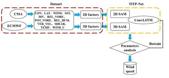
Figure 2 demonstrates how we used multidimensional variables to create a comprehensive typhoon intensity environmental field to extract the temporal and spatial correlations between the various impact components. The dataset is chronologically divided into two parts: training data (dataset from 2001–2014) and test data (dataset from 2015–2018).
To prevent network convergence failure, the dataset is normalized before training the model to unify the unit of measurement. Normalized data processing can speed up the process of finding the best gradient descent solution and enhance forecast accuracy.
Equation (1) shows the dataset normalization method used in the paper. Additionally, the data are denormalized using Equation (2) after training the model.
In Equations (1) and (2), is the value after normalization, is the value before normalization, and and are the minimum and maximum values in the group.
3. Methods
This section focuses on the details of the TITP-Net hybrid model.
Section 3.1 explains how spatial features are extracted from the environmental disturbance using the SAM.
Section 3.2 introduces learning the spatio-temporal information of typhoon intensity and environmental disturbance using ConvLSTM.
Section 3.3 displays the rolling forecasting method.
Section 3.4 summarizes the overall framework of TITP-Net hybrid model.
Section 3.5 indicates the model evaluation metrics.
3.1. Learning Spatial Features of Multidimensional Environmental Factors by Using a Spatial Attention Module
Typhoon intensity is affected by many factors and making full use of multidimensional factors will improve typhoon intensity forecasting performance. Integrating multidimensional variables into a dataset is conducive to improving intensity predictions. Previous research has shown that fully connected and convolution processes may extract features effectively [
43]. In this paper, we propose a spatial attention module (SAM) to capture the spatial relationship between variables, as shown in
Figure 3. Multidimensional factors determining typhoon intensity are taken into account, and several feature extraction approaches are utilized for various dimensional data. The typhoon intensity environmental field is input to the SAM, and 2DConv is used to extract spatial features from 2D data such as SST and REL_HUM, whereas 3DConv is utilized to extract features from 3D data. At time t, the SAM receives
,
and
as input for stressing crucial areas, as shown in Equations (3)–(5):
where
and
are 2D atmospheric factors and 2D ocean factors, respectively,
is the 3D atmospheric factor, and SAM is the spatial attention module.
,
and
are refined features, which are calculated using Equations (6)–(11).
For 2D atmospheric factors , a MaxPool2d operation and an AvgPool2d operation are adopted to generate two 2D maps and . Next, after two 2DConv operations, a 2D spatial map is fused and input to a MaxPool2d operation and an AvgPool2d operation to generate two 2D maps and . Finally, the refined feature is fused by two 2DConv operations, as shown in Equations (6) and (7). Similarly, Equations (8) and (9) are applied to 3D atmospheric factors, and the spatial attention features of 2D ocean factors are calculated using Equations (10) and (11).
3.2. Learn the Spato-Temporal Feature of Large-Scale Environmental Factors by Using ConvLSTM
To learn the spatio-temporal relationships of multidimensional variables, a ConvLSTM network is used. ConvLSTM was first proposed to solve the precipitation proximity prediction problem [
44]. It can not only establish temporal relations as LSTM but can also describe local spatial features as a convolutional neural network (CNN). In terms of obtaining spatio-temporal relations, ConvLSTM outperforms both LSTM and CNN-LSTM. The method replaces the input-to-state and state-to-state parts of LSTM with the form of convolution by feedforward calculation. The connection between the input and each gate is replaced by feedforward convolution, and the operation between states is also changed. With the addition of the convolution operation, not only tempo-relation can be obtained but also spatial features can be effectively extracted, similar to the convolution layer. ConvLSTM has been used to solve a variety of temporal and spatial challenges, including precipitation forecasting. The calculation of ConvLSTM is shown in Equations (12)–(17).
where
is the input at time t;
represents the network output;
represents the candidate values of the storage unit status;
is the weight matrix and
represents the deviation vector matrix;
is the multiplication of the corresponding elements of the matrix, also known as the Hadamard product;
denotes the convolution operation;
represents the value of the input gate, and
represents the value of the output gate;
stands for memory cells, which not only retain the current input features but also control whether the previous moment of information continues to pass;
is the hyperbolic tangent function; and
represents the sigmoid function.
3.3. Rolling Forecast Method
Forecasting methods based on deep learning include single-step prediction and multistep prediction. Most previous studies on TC intensity prediction using deep learning approaches produced single-step predictions [
13,
15]. The single-step method can only provide prediction at a particular lead time and cannot efficiently capture the detailed evolution of TCs. Multistep prediction can predict values with long lead time, although with increasing prediction error as time step increases. In simple multistep prediction, numerous environmental variables are used for predicting TC intensity, and only output TC intensity in the next few time steps [
27]. As a result, simple multistep prediction cannot catch the relevance of the two adjacent prediction values. To overcome this problem, we adopt a modified multistep approach, the rolling prediction method, which predicts not only typhoon intensity but also environmental variables in the future time steps and then uses the predicted environmental variables to further make prediction until the target time step.
The length of input time steps is defined as sequence length. Next, in the rolling prediction method, the TITP-Net model uses the environmental data and typhoon wind speed of a particular sequence length to forecast the environmental data and typhoon wind speed step by step. Assuming present time is t, we use the input spatio-temporal matrix (s=1, 2, 3…, sequence length) to predict , then combine the predicted and as a new input spatio-temporal matrix to predict , and repeat it similarly until (p =1, 2, 3…, target time step). Through the above process, the typhoon wind speed can be obtained with lead times of 6 h (p = 1), 12 h (p = 2), 18 h (p = 3), 24 h (p = 4) or even longer (p > 4).
3.4. Framework of the Hybrid TITP-Net
The overall framework of TITP-Net is shown in
Figure 4. The model is built with ConvLSTM and a SAM. As described in
Section 3.1, the input
consists of 2D atmospheric data, 3D atmospheric data and 2D ocean data, which can be expressed as
= [
,
,
]. In the SAM, 2DConv is adopted to extract features from [
], while 3DConv is adopted to extract features from [
], learning the spatial features of atmospheric and oceanic data.
The variables at time t are combined to fuse
. Next,
is input to ConvLSTM to captive the spatio-temporal data matrix for further forecasting. The detailed operation is shown in
Section 3.1,
Section 3.2 and
Section 3.3 and is summarized as Equation (18):
where TITP-Net represents the proposed model,
is the fused input matrix,
are predicted values, and
is the predicted result at the target time step
p.
3.5. Evaluation Metrics
The model performance is evaluated based on two widely employed classic error criteria, the mean value of the absolute errors (MAE) and the root mean square error (RMSE). These two metrics are defined as follows:
where
is the true value of the ith timestep;
is the prediction value; and
is the number of samples. Both the MAE and RMSE are used to measure the deviation between the true value and the predicted value. The performance is better if the values of the MAE and RMSE are smaller.
4. Experimental Results
4.1. Results with Different Sequence Lengths
Input sequence length is an important parameter for learning spatio-temporal features, and different sequence lengths will result in various forecasting errors.
Figure 5 demonstrates the 24 h (
p = 4, see
Section 3.3) forecasting results of different sequence lengths from 2015–2018. Considering the demand of timely predicting typhoon intensity, we use the 6 h (s = 1), 12 h (s = 2), 18 h (s = 3) and 24 h (s = 4) typhoon records as input and compare the model prediction performance at different sequence lengths. Overall, inputting 24 h (s = 4) data achieves the best performance among the 4 sequence lengths we considered. Take 2015 as an example, the MAE results for sequence length of 6 h, 12 h, 18 h, and 24 h are 7.76 m/s, 7.04 m/s, 4.51 m/s, and 3.87 m/s, respectively, and the RMSE results are 10.20 m/s, 9.80 m/s, 6.22 m/s and 5.65 m/s, respectively. From 2015 to 2018, when inputting 6 h (s = 1) typhoon records, the MAEs are 7.76 m/s, 8.64 m/s, 7.30 m/s and 7.50 m/s. When inputting 24 h (s = 4) typhoon records, the model obtains better performance with MAEs of 3.87 m/s, 4.61 m/s, 3.60 m/s and 3.90 m/s. With more records input, the model can learn more data features and obtain more accurate results. The average MAE and RMSE of inputting 24 h (s = 4) typhoon records are 3.98 m/s and 6.32 m/s, respectively, which are smaller than the others in most cases.
4.2. Results with Different Learning Rates
The learning rate (Lr) determines whether and when the objective function converges to the local minimum. With an appropriate learning rate, the objective function can converge to the local minimum in the shortest amount of time.
Figure 6 shows the model performance based on different Lrs from 2015–2018. As shown in
Figure 6a, when Lr is 0.0001, the MAE results are 3.87 m/s, 4.61 m/s, 3.6 m/s and 3.9 m/s from 2015 to 2018, and the four-year average MAE is 3.98 m/s, which is smaller than the other learning rates. From
Figure 6b, it can be seen that the RMSE results of the model are minimal when the learning rate is 0.0001, and the four-year average RMSE is 6.32 m/s. Therefore, the best Lr for the model is 0.0001 based on our examination.
4.3. Results with Different Optimizers
The optimizer is a crucial step for deep learning, and it is used to minimize (or maximize) the loss function by updating and calculating network parameters that affect model training and model output to approximate or reach optimal values. If a poor optimizer is chosen, it will have a great impact on the model results and dampen the learning efficiency. Some common optimizers are considered in this study, including stochastic gradient descent (SGD) [
45], Root Mean Square prop (RMSprop) [
46], AdaGrad [
47], AdaDelta [
48], adaptive moment estimation (Adam) [
46,
49,
50] and AdaMax [
50,
51,
52].
Figure 7 illustrates the typhoon intensity forecasting results with different optimizers over 24 h. From
Figure 7a, the MAE of the model with the Adam optimizer has the best performance in 2015, 2017 and 2018, which are 3.87 m/s, 3.60 m/s and 3.90 m/s, respectively. The four-year forecasting average MAE with the Adam optimizer is 3.98 m/s, which is an improvement of 5.01% over the second-best performance. From
Figure 7b, the RMSE of the model with the Adam optimizer has the best performance in 2015 and 2017, which are 5.65 m/s and 5.89 m/s, respectively. The four-year forecasting average RMSE is 6.32 m/s, which is an improvement of 1.56% over the second-best performance. In plain words, Adam is suitable for typhoon intensity forecasting. The best performance of the Adam optimizer is mainly because Adam is the combination of Adaptive Gradient (AdaGrad) and RMSprop, which basically solves a series of problems of gradient descent, such as a random small sample, adaptive learning rate, and easy to become stuck in the point of a small gradient.
4.4. Results with Different Epochs
The epoch represents the dataset training time, which is critical for typhoon intensity forecasting. If the dataset passes too few times through the neural network, it will be underfit; otherwise, if it is passed too many times, it will be overfit.
Figure 8 demonstrates the forecasting results in 24 h with the change in epochs based on the TITP-Net model. After 500 epochs, the model may be overfit. Therefore, the epochs range from 100 to 500, and the decrease rate is 100. After training the model with 300 epochs, the four-year average MAE and RMSE in 24 h are 3.98 m/s and 6.32 m/s, respectively. With 400 epochs, the four-year average MAE and RMSE in 24 h are 4.06 m/s and 6.35 m/s, respectively. The TITP-Net model achieved the best performance based on 300 epochs compared to 400 epochs. Therefore, using 300 epochs is suitable for training the model.
5. Results for Typhoon Intensity Forecasting
We used two types of baselines to validate the performance of the proposed TITP-Net model. One is other machine learning methods, and the other is up-to-date typhoon intensity forecasting reports from official agencies.
Section 5.1 compares the results of some common deep learning models with the TITP-Net performance in 24 h prediction.
Section 5.2 uses some prediction reports and some new forecasting results as baselines to evaluate the performance of the TITP-Net model in 24 h prediction.
Section 5.3 demonstrates the typhoon intensity prediction performance in other timesteps, including 6 h, 12 h, 18 h, 24 h, 36 h and 48 h.
5.1. Performance Analysis of Various Deep Learning Models
To verify the proposed model effectiveness and practicability, some common deep learning models are introduced to the experiment, including LSTM, Stack-LSTM, Bi-LSTM, CNN-LSTM, CNN-GRU and ConvLSTM, as shown in
Figure 9. Among these models, the CNN-LSTM and CNN-GRU models achieve the worst performance. The major cause is that the two models are originally designed for single-step prediction without considering multistep prediction using factor dependencies, which cannot balance the results among multiple prediction intervals. The performance results of the LSTM, Stack LSTM and Bi-LSTM models are better than those of the CNN-LSTM and CNN-GRU models but worse than those of the TITP-Net model. The main reason here is that LSTM cannot capture typhoon spatial features effectively. The TITP-Net model outperforms the second-best performance ConvLSTM, with MAE improvements of 13.62%, 2.95%, and 3.94% and RMSE improvements of 10.03%, 2.72%, and 6.09% in 2015, 2016 and 2018, respectively. Comparing the four-year average forecasting error with those models, the proposed TITP-Net model achieved a better performance with MAE improvements of 25.75%, 25.33%, 22.72%, 64.72%, 64.01% and 4.56% and RMSE improvements of 19.90%, 18.97%, 11.11%, 55.62%, 55.68% and 4.53% than those models. Overall, the results of TITP-Net demonstrate that it can effectively utilize the information from the sequence of environmental variables and the relationship of multidimensional variables to improve the accuracy and performance of typhoon intensity prediction.
5.2. The Results of Different Methods in 24 h Prediction from 2015–2018
In this Section, we utilize WMO Typhoon Committee 2015 [
53], WMO Typhoon Committee 2016 [
54], WMO Typhoon Committee 2017 [
55], and WMO Typhoon Committee 2018 [
56], released by an institution named the Typhoon Committee, which is jointly held by the Economic and Social Commission for Asia and the Pacific (ESCAP) and the World Meteorological Organization (WMO). We select the official guidance, including from the CMA, JMA, Korea Meteorological (KMA) and Hong Kong Observatory (HKO); global models, including the Integrated Forecasting System of European Centre for Medium Range Weather Forecasting (ECMWF-IFS), Global Forecast System of National Centers for Environmental Prediction (NCEP-GFS) and Global Spectral Model of Japan Meteorological Agency (JMA-GSM); and regional models, including the Tropical cyclone model in the Australian Community Climate and Earth-System Simulator Numerical Weather Prediction systems (BoM-ACCESS-TC) and Tropical Regional Atmosphere Model for the South China Sea based on GRAPES (CMA-TRAMS) as the baselines. To further compare the accuracy of typhoon intensity prediction by the model, we quoted Xu’s experimental results, and the typhoon intensity prediction errors based on the proposed SAF-Net model at a lead time of 24 h in 2015, 2016, 2017 and 2018 were 4.54 m/s, 4.78 m/s, 3.95 m/s and 3.94 m/s, respectively [
26].
The MAE results of different methods are shown in
Figure 10. We compare the annual forecast results of different WMO methods and select the lowest error as the WMO prediction accuracy. The minimum MAEs of typhoon intensity prediction from 2015 to 2018 are 4.26 m/s for the CMA, 5.1 m/s for the CMA, 4.91 m/s for the HKO and 3.90 m/s for the JMA, and the four-year average forecasting minimum error is 4.73 m/s for the CMA. In detail, the proposed model does not improve the typhoon prediction at a lead time of 24 h in 2018 but outperforms the typhoon prediction of the WMO from 2015 to 2017, with improvements of 9.15%, 9.61% and 26.68%. The four-year average prediction error is 15.86% lower than the WMO.
Next, we compare the results with a recent deep learning method, SAF-Net. The SAF-Net model obtains better results, with improvements of 6.27% and 19.55% in 2016 and 2017, respectively, and a mean improvement of 9.09% over the WMO. However, the proposed TITP-Net still outperforms SAF-Net, improving the forecasting accuracy by 14.76% in 2015, 3.56% in 2016, 8.86% in 2017, 1.02% in 2018 and 7.44% on average. In general, the TITP-Net model can outperform other methods in typhoon intensity prediction.
5.3. Comparison of the MAEs with Different Lead Times
To comprehensively compare the prediction performance of the model with different lead times (target time steps,
p), we further compare the proposed model with the results from official agencies and deep learning models of other scholars in 6 h (
p = 1), 12 h (
p = 2), 18 h (
p = 3), 24 h (
p = 4), 36 h (
p = 6), and 48 h (
p = 8) predictions. The objective models of official agencies, the National Hurricane Center (NHC) [
57,
58], JTWC [
59] and Hurricane Weather Research and Forecasting (HWRF) [
58], are used as the agency baselines to illustrate the practical usability of the proposed model. The results of previous studies are also used as deep learning model baselines to verify its effectiveness, including LSTM-8 [
24] and FFNN [
58]. The prediction errors of these methods are shown in
Figure 11. Evaluation of the MAE metrics of official agencies and other scholar results in 6 h, 12 h, 18 h, 24 h, 36 h and 48 h prediction. Each point represents the forecasting MAE at 6–48 h by different methods. The red point plot represents the results in various hours prediction of TITP-Net. The result of the 6 h prediction using LSTM-8 is slightly better than the results of the official agencies. In the 12 h prediction, the JTWC has the best performance, with an improvement of 8.65% compared to the second-best result. In the 18 h, 24 h, 36 h and 48 h predictions, our model achieves better performance, with values of 7.02%, 6.53%, 6.25% and 5.37%, respectively, compared with the second-best prediction. In summary, the results show that the performance based on TITP-Net is better with longer lead times.
6. Conclusions
In this paper, typhoon intensity forecasting is treated as a spatio-temporal regression prediction problem in the deep learning field. Some studies have proven that integrating different dimension variables into a dataset can better understand typhoon formation and promise for improving intensity prediction. We propose a novel spatial attention module that includes 2DConv, which is used to capture features in 2D variables, and 3DConv, which is used to capture features in 3D variables. Next, a novel spatio-temporal forecasting model named TITP-Net is developed, with the ConvLSTM and spatial attention module to capture the local correlated features.
TITP-Net is trained and tested using historical typhoon information records from 2001–2018, including typhoon location and intensity from CMA, multidimensional environmental variable datasets form ECMWF. To enable model training, extensive experiments are carried out to choose the optimal model parameters: the optimal input sequence length is 4; the optimal learning rate is 0.0001; the optimal optimizer for improving model performance is Adam; and, finally, the optimal epoch is 300 epochs. The results in the 24 h prediction are 3.87 m/s in 2015, 4.61 m/s in 2016, 3.60 m/s in 2017, 3.90 m/s in 2018 and 3.98 m/s in the four-year average.
Next, we compare our model with various methods to evaluate its performance. We introduce two types of baselines, machine learning methods and up-to-date typhoon intensity forecasting reports. Compared with machine learning methods in 24 h prediction, the TITP-Net model outperforms the other models, with an MAE improvement of 4.56% and RMSE improvement of 4.53% compared to ConvLSTM. Next, the up-to-date typhoon intensity forecasting reports are regarded as the second baselines, including the typhoon intensity forecasting reports and the recent SAF-Net deep learning method. Our model achieves the best performance, with improvements of 9.15%, 9.61%, and 26.68% in 2015–2017 and 15.86% in mean error compared to the WMO. Compared to SAF-Net, TITP-Net improves the forecasting accuracy by 14.76% in 2015, 3.56% in 2016, 8.86% in 2017, 1.02% in 2018 and 7.44% on average. In general, our proposed model outperforms the baselines.
Finally, we further compare our proposed model with the results from official agencies and the deep learning models of previous studies in 6 h, 12 h, 18 h, 24 h, 36 h and 48 h prediction. The model outperforms the baselines at 18 h, 24 h, 36 h and 48 h lead times, with improvements of 7.02%, 6.53%, 6.25% and 5.37% compared to the second-best prediction.
Our proposed model improves the prediction of typhoon intensity by fully extracting the information from the massive data with a proper method and framework. However, some further work should be carried out in the future. First, we may further make an improvement in the short-term prediction (6 h and 12 h) of typhoon intensity. Second, a more novel network based on a ConvGRU and ST-LSTM may enable a better prediction, which should be adopted in future research.


