
Estimating PM2.5 Concentrations Using the Machine Learning RF-XGBoost Model in Guanzhong Urban Agglomeration, China

 , ,
, ,
Abstract
:
1. Introduction
2. Materials and Methods
2.1. Study Area
2.2. Data Source
2.2.1. Ground Measurements
2.2.2. MODIS AOD
2.2.3. Meteorological Conditions
2.2.4. Auxiliary Data
2.3. Methodology
2.3.1. Data Integration
2.3.2. Fill Missing AOD with RF
2.3.3. XGBoost Model and Feature Selection
2.3.4. Model Evaluation
3. Results
3.1. Model Performance of RF
3.2. Statistics of Variables
3.3. Model Performance of XGBoost
3.3.1. Reginal-Scale Model Performance
3.3.2. Seasonal Model Performance
3.3.3. Site-Scale Model Performance
3.4. Model Prediction of XGBoost
3.5. Seasonal and Annual Distribution of PM2.5
4. Discussion
4.1. RF-XGBoost Model Performances
4.2. Comparision with Other Ensemble Models
4.3. Reasons for PM2.5 Pollution in the GZB
5. Conclusions
Author Contributions
Funding
Data Availability Statement
Acknowledgments
Conflicts of Interest
References
- Lelieveld, J.; Evans, J.S.; Fnais, M.; Giannadaki, D.; Pozzer, A. The contribution of outdoor air pollution sources to premature mortality on a global scale. Nature 2015, 525, 367–371. [Google Scholar] [CrossRef] [PubMed]
- Lu, D.; Xu, J.; Yue, W.; Mao, W.; Yang, D.; Wang, J. Response of PM2.5 pollution to land use in China. J. Clean. Prod. 2019, 244, 118741. [Google Scholar] [CrossRef]
- Rushingabigwi, G.; Nsengiyumva, P.; Sibomana, L.; Twizere, C.; Kalisa, W. Analysis of the atmospheric dust in Africa: The breathable dust’s fine particulate matter PM2.5 in correlation with carbon monoxide. Atmos. Environ. 2020, 224, 117319. [Google Scholar] [CrossRef]
- Li, G.; Fang, C.; Wang, S.; Sun, S. The Effect of Economic Growth, Urbanization, and Industrialization on Fine Particulate Matter (PM2.5) Concentrations in China. Environ. Sci. Technol. 2016, 50, 11452–11459. [Google Scholar] [CrossRef] [PubMed]
- China National Environmental Monitoring Centre. Notice About Monitoring According to National Air Monitoring Net “12th Five-Year Plan”. 2012. Available online: http://www.cnemc.cn/gzdt/wjtz/201204/t20120419_648459.shtml (accessed on 15 March 2022). (In Chinese).
- Chinese State Council. National Environment Protection “12th Five-Year Plan”. 2011. Available online: http://www.gov.cn/zwgk/2011-12/20/content_2024895.htm (accessed on 15 March 2022). (In Chinese)
- Chinese State Council. Action Plan on Air Pollution Prevention and Control. 2013. Available online: http://www.gov.cn/zwgk/2013-09/12/content_2486773.htm (accessed on 15 March 2022). (In Chinese)
- Chinese State Council. Three-Year Action Plan on Defending the Blue Sky. 2018. Available online: http://www.gov.cn/zhengce/content/2018-07/03/content_5303158.htm (accessed on 15 March 2022). (In Chinese)
- Chen, T.; Guestrin, C. XGBoost. In Proceedings of the 22nd ACM SIGKDD International Conference on Knowledge Discovery and Data Mining—KDD’16, San Francisco, CA, USA, 13–17 August 2016; pp. 785–794. [Google Scholar]
- Ministry of Ecology and Environment the People’s Republic of China. 2020 Bulletin of China’s Ecological Environment. 2021. Available online: https://www.mee.gov.cn/hjzl/sthjzk/zghjzkgb/202105/P020210526572756184785.pdf (accessed on 15 March 2022). (In Chinese)
- Sorek-Hamer, M.; Chatfield, R.; Liu, Y. Review: Strategies for using satellite-based products in modeling PM2.5 and short-term pollution episodes. Environ. Int. 2020, 144, 106057. [Google Scholar] [CrossRef] [PubMed]
- Xu, Y.; Ho, H.C.; Wong, M.S.; Deng, C.; Shi, Y.; Chan, T.C.; Knudby, A. Evaluation of machine learning techniques with multiple remote sensing datasets in estimating monthly concentrations of ground-level PM2.5. Environ. Pollut. 2018, 242 Pt B, 1417–1426. [Google Scholar] [CrossRef]
- Zuo, X.; Guo, H.; Shi, S.; Zhang, X. Comparison of Six Machine Learning Methods for Estimating PM2.5 Concentration Using the Himawari-8 Aerosol Optical Depth. J. Indian Soc. Remote Sens. 2020, 48, 1277–1287. [Google Scholar] [CrossRef]
- Li, J.; Garshick, E.; Hart, J.E.; Li, L.; Shi, L.; Al-Hemoud, A.; Huang, S.; Koutrakis, P. Estimation of ambient PM2.5 in Iraq and Kuwait from 2001 to 2018 using machine learning and remote sensing. Environ. Int. 2021, 151, 106445. [Google Scholar] [CrossRef]
- Zhang, D.; Du, L.; Wang, W.; Zhu, Q.; Bi, J.; Scovronick, N.; Naidoo, M.; Garland, R.M.; Liu, Y. A machine learning model to estimate ambient PM2.5 concentrations in industrialized highveld region of South Africa. Remote Sens. Environ. 2021, 266, 112713. [Google Scholar] [CrossRef]
- Chen, J.; Yin, J.; Zang, L.; Zhang, T.; Zhao, M. Stacking machine learning model for estimating hourly PM2.5 in China based on Himawari 8 aerosol optical depth data. Sci. Total Environ. 2019, 697, 134021. [Google Scholar] [CrossRef]
- Joharestani, M.Z.; Cao, C.; Ni, X.; Bashir, B.; Talebiesfandarani, S. PM2.5 Prediction Based on Random Forest, XGBoost, and Deep Learning Using Multisource Remote Sensing Data. Atmosphere 2019, 10, 373. [Google Scholar] [CrossRef] [Green Version]
- Just, A.C.; De Carli, M.M.; Shtein, A.; Dorman, M.; Lyapustin, A.; Kloog, I. Correcting Measurement Error in Satellite Aerosol Optical Depth with Machine Learning for Modeling PM2.5 in the Northeastern USA. Remote Sens. 2018, 10, 803. [Google Scholar] [CrossRef] [Green Version]
- Tian, H.; Zhao, Y.; Luo, M.; He, Q.; Han, Y.; Zeng, Z. Estimating PM2.5 from multisource data: A comparison of different machine learning models in the Pearl River Delta of China. Urban Clim. 2020, 35, 100740. [Google Scholar] [CrossRef]
- Zeng, Z.; Gui, K.; Wang, Z.; Luo, M.; Geng, H.; Ge, E.; An, J.; Song, X.; Ning, G.; Zhai, S.; et al. Estimating hourly surface PM2.5 concentrations across China from high-density meteorological observations by machine learning. Atmospheric Res. 2021, 254, 105516. [Google Scholar] [CrossRef]
- Zheng, T.; Bergin, M.H.; Hu, S.; Miller, J.; Carlson, D.E. Estimating ground-level PM2.5 using micro-satellite images by a convolutional neural network and random forest approach. Atmos. Environ. 2020, 230, 117451. [Google Scholar] [CrossRef]
- Di, Q.; Kloog, I.; Koutrakis, P.; Lyapustin, A.; Wang, Y.; Schwartz, J. Assessing PM2.5 Exposures with High Spatiotemporal Resolution across the Continental United States. Environ. Sci. Technol. 2016, 50, 4712–4721. [Google Scholar] [CrossRef] [PubMed] [Green Version]
- Sun, K.; Tang, L.; Qian, J.; Wang, G.; Lou, C. A deep learning-based PM2.5 concentration estimator. Displays 2021, 69, 102072. [Google Scholar] [CrossRef]
- Li, X.; Zhang, X. Predicting ground-level PM2.5 concentrations in the Beijing-Tianjin-Hebei region: A hybrid remote sensing and machine learning approach. Environ. Pollut. 2019, 249, 735–749. [Google Scholar] [CrossRef] [Green Version]
- Wei, J.; Li, Z.; Cribb, M.; Huang, W.; Xue, W.; Sun, L.; Guo, J.; Peng, Y.; Li, J.; Lyapustin, A.; et al. Improved 1 km resolution PM2.5 estimates across China using enhanced space–time extremely randomized trees. Atmos. Chem. Phys. 2020, 20, 3273–3289. [Google Scholar] [CrossRef] [Green Version]
- Wei, J.; Huang, W.; Li, Z.; Xue, W.; Peng, Y.; Sun, L.; Cribb, M. Estimating 1-km-resolution PM2.5 concentrations across China using the space-time random forest approach. Remote Sens. Environ. 2019, 231, 111221. [Google Scholar] [CrossRef]
- Chen, W.; Ran, H.; Cao, X.; Wang, J.; Teng, D.; Chen, J.; Zheng, X. Estimating PM2.5 with high-resolution 1-km AOD data and an improved machine learning model over Shenzhen, China. Sci. Total Environ. 2020, 746, 141093. [Google Scholar] [CrossRef] [PubMed]
- Chen, B.; Song, Z.; Pan, F.; Huang, Y. Obtaining vertical distribution of PM2.5 from CALIOP data and machine learning algorithms. Sci. Total Environ. 2021, 805, 150338. [Google Scholar] [CrossRef] [PubMed]
- Lyapustin, A.; Wang, Y.; Korkin, S.; Huang, D. MODIS Collection 6 MAIAC algorithm. Atmospheric Meas. Tech. 2018, 11, 5741–5765. [Google Scholar]
- Paciorek, C.J.; Liu, Y. Limitations of remotely sensed aerosol as a spatial proxy for fine particulate matter. Environ. Health Perspect. 2009, 117, 904–909. [Google Scholar] [CrossRef] [PubMed] [Green Version]
- Just, A.C.; Wright, R.O.; Schwartz, J.; Coull, B.A.; Baccarelli, A.A.; Tellez-Rojo, M.M.; Moody, E.; Wang, Y.; Lyapustin, A.; Kloog, I. Using High-Resolution Satellite Aerosol Optical Depth To Estimate Daily PM2.5 Geographical Distribution in Mexico City. Environ. Sci. Technol. 2015, 49, 8576–8584. [Google Scholar] [CrossRef] [Green Version]
- Wei, J.; Li, Z.; Guo, J.; Sun, L.; Huang, W.; Xue, W.; Fan, T.; Cribb, M. Satellite-Derived 1-km-Resolution PM1 Concentrations from 2014 to 2018 across China. Environ. Sci. Technol. 2019, 53, 13265–13274. [Google Scholar] [CrossRef]
- Chew, B.N.; Campbell, J.R.; Salinas, S.V.; Chang, C.W.; Reid, J.S.; Welton, E.J.; Holben, B.N.; Liew, S.C. Aerosol particle vertical distributions and optical properties over Singapore. Atmospheric Environ. 2013, 79, 599–613. [Google Scholar] [CrossRef]
- Madhavan, B.L.; Niranjan, K.; Sreekanth, V.; Sarin, M.M.; Sudheer, A.K. Aerosol characterization during the summer monsoon period over a tropical coastal Indian station, Visakhapatnam. J. Geophys. Res. 2008, 113. [Google Scholar] [CrossRef] [Green Version]
- Zhang, H.; Wang, Y.; Hu, J.; Ying, Q.; Hu, X.M. Relationships between meteorological parameters and criteria air pollutants in three megacities in China. Environ. Res. 2015, 140, 242–254. [Google Scholar] [CrossRef]
- Monforte, P.; Ragusa, M.A. Temperature Trend Analysis and Investigation on a Case of Variability Climate. Mathematics 2022, 10, 2202. [Google Scholar] [CrossRef]
- Fan, Y.; van den Dool, H. A global monthly land surface air temperature analysis for 1948–present. J. Geophys. Res. Atmos. 2008, 113, D01103. [Google Scholar] [CrossRef]
- Han, Y.; Xu, H.; Zheng, C.; Liu, P. Particulate matters emitted from maize straw burning for winter heating in rural areas in Guanzhong Plain, China: Current emission and future reduction. Atmospheric Res. 2017, 184, 66–76. [Google Scholar]
- Liu, Y.; Paciorek, C.J.; Koutrakis, P. Estimating regional spatial and temporal variability of PM(2.5) concentrations using satellite data, meteorology, and land use information. Environ. Health Perspect 2009, 117, 886–892. [Google Scholar] [CrossRef] [PubMed] [Green Version]
- Breiman, L. Random Forests. Mach. Learn. 2001, 45, 5–32. [Google Scholar] [CrossRef] [Green Version]
- Akritidis, D.; Zanis, P.; Georgoulias, A.K.; Papakosta, E.; Tzoumaka, P.; Kelessis, A. Implications of COVID-19 Restriction Measures in Urban Air Quality of Thessaloniki, Greece: A Machine Learning Approach. Atmosphere 2021, 12, 1500. [Google Scholar] [CrossRef]
- Aljanabi, M.; Shkoukani, M.; Hijjawi, M. Ground-level Ozone Prediction Using Machine Learning Techniques: A Case Study in Amman, Jordan. Int. J. Autom. Comput. 2020, 17, 667–677. [Google Scholar] [CrossRef]
- Keller, C.A.; Evans, M.J.; Knowland, K.E.; Hasenkopf, C.A.; Modekurty, S.; Lucchesi, R.A.; Oda, T.; Franca, B.B.; Mandarino, F.C.; Díaz Suárez, M.V.; et al. Global impact of COVID-19 restrictions on the surface concentrations of nitrogen dioxide and ozone. Atmos. Chem. Phys. 2021, 21, 3555–3592. [Google Scholar] [CrossRef]
- Sun, Y.; Yin, H.; Lu, X.; Notholt, J.; Palm, M.; Liu, C.; Tian, Y.; Zheng, B. The drivers and health risks of unexpected surface ozone enhancements over the Sichuan Basin, China, in 2020. Atmos. Chem. Phys. 2021, 21, 18589–18608. [Google Scholar] [CrossRef]
- Wang, J.; He, L.; Lu, X.; Zhou, L.; Tang, H.; Yan, Y.; Ma, W. A full-coverage estimation of PM2.5 concentrations using a hybrid XGBoost-WD model and WRF-simulated meteorological fields in the Yangtze River Delta Urban Agglomeration, China. Environ. Res. 2022, 203, 111799. [Google Scholar] [CrossRef]
- Gui, K.; Che, H.; Zeng, Z.; Wang, Y.; Zhai, S.; Wang, Z.; Luo, M.; Zhang, L.; Liao, T.; Zhao, H.; et al. Construction of a virtual PM2.5 observation network in China based on high-density surface meteorological observations using the Extreme Gradient Boosting model. Environ. Int. 2020, 141, 105801. [Google Scholar] [CrossRef]
- Fu, D.; Song, Z.; Zhang, X.; Xia, X.; Wang, J.; Che, H.; Wu, H.; Tang, X.; Zhang, J.; Duan, M. Mitigating MODIS AOD non-random sampling error on surface PM2.5 estimates by a combined use of Bayesian Maximum Entropy method and linear mixed-effects model. Atmos. Pollut. Res. 2020, 11, 482–490. [Google Scholar] [CrossRef]
- He, W.; Meng, H.; Han, J.; Zhou, G.; Zheng, H.; Zhang, S. Spatiotemporal PM2.5 estimations in China from 2015 to 2020 using an improved gradient boosting decision tree. Chemosphere 2022, 296, 134003. [Google Scholar] [CrossRef] [PubMed]
- He, Q.; Gu, Y.; Zhang, M. Spatiotemporal trends of PM2.5 concentrations in central China from 2003 to 2018 based on MAIAC-derived high-resolution data. Environ. Int. 2020, 137, 105536. [Google Scholar] [CrossRef] [PubMed]
- Chen, G.; Li, Y.; Zhou, Y.; Shi, C.; Guo, Y.; Liu, Y. The comparison of AOD-based and non-AOD prediction models for daily PM2.5 estimation in Guangdong province, China with poor AOD coverage. Environ. Res. 2021, 195, 110735. [Google Scholar] [CrossRef] [PubMed]
- Zhang, P.; Ma, W.; Wen, F.; Liu, L.; Yang, L.; Song, J.; Wang, N.; Liu, Q. Estimating PM2.5 concentration using the machine learning GA-SVM method to improve the land use regression model in Shaanxi, China. Ecotoxicol. Environ. Saf. 2021, 225, 112772. [Google Scholar] [CrossRef] [PubMed]
- Nabavi, S.O.; Haimberger, L.; Abbasi, E. Assessing PM2.5 concentrations in Tehran, Iran, from space using MAIAC, deep blue, and dark target AOD and machine learning algorithms. Atmos. Pollut. Res. 2018, 10, 889–903. [Google Scholar] [CrossRef]
- Bagheri, H. A machine learning-based framework for high resolution mapping of PM2.5 in Tehran, Iran, using MAIAC AOD data. Adv. Space Res. 2022, 69, 3333–3349. [Google Scholar] [CrossRef]
- Ghahremanloo, M.; Choi, Y.; Sayeed, A.; Salman, A.K.; Pan, S.; Amani, M. Estimating daily high-resolution PM2.5 concentrations over Texas: Machine Learning approach. Atmospheric Environ. 2021, 247, 118209. [Google Scholar] [CrossRef]
- Goldberg, D.L.; Gupta, P.; Wang, K.; Jena, C.; Zhang, Y.; Lu, Z.; Streets, D.G. Using gap-filled MAIAC AOD and WRF-Chem to estimate daily PM2.5 concentrations at 1 km resolution in the Eastern United States. Atmos. Environ. 2019, 199, 443–452. [Google Scholar] [CrossRef]
- Pu, Q.; Yoo, E.-H. Ground PM2.5 prediction using imputed MAIAC AOD with uncertainty quantification. Environ. Pollut. 2021, 274, 116574. [Google Scholar] [CrossRef]
- Kloog, I.; Chudnovsky, A.A.; Just, A.C.; Nordio, F.; Koutrakis, P.; Coull, B.A.; Lyapustin, A.; Wang, Y.; Schwartz, J. A New Hybrid Spatio-Temporal Model For Estimating Daily Multi-Year PM2.5 Concentrations Across Northeastern USA Using High Resolution Aerosol Optical Depth Data. Atmos. Environ. 2014, 95, 581–590. [Google Scholar] [CrossRef] [PubMed] [Green Version]
- Di, Q.; Amini, H.; Shi, L.; Kloog, I.; Silvern, R.; Kelly, J.; Sabath, M.B.; Choirat, C.; Koutrakis, P.; Lyapustin, A. An ensemble-based model of PM2.5 concentration across the contiguous United States with high spatiotemporal resolution. Environ. Int. 2019, 130, 104909. [Google Scholar] [CrossRef] [PubMed]
- Just, A.C.; Arfer, K.B.; Rush, J.; Dorman, M.; Shtein, A.; Lyapustin, A.; Kloog, I. Advancing methodologies for applying machine learning and evaluating spatiotemporal models of fine particulate matter (PM2.5) using satellite data over large regions. Atmos. Environ. 2020, 239, 117649. [Google Scholar] [CrossRef] [PubMed]
- Li, L.; Zhang, J.; Meng, X.; Fang, Y.; Ge, Y.; Wang, J.; Wang, C.; Wu, J.; Kan, H. Estimation of PM2.5 concentrations at a high spatiotemporal resolution using constrained mixed-effect bagging models with MAIAC aerosol optical depth. Remote Sens. Environ. 2018, 217, 573–586. [Google Scholar] [CrossRef]
- Nie, D.; Shen, F.; Wang, J.; Ma, X.; Li, Z.; Ge, P.; Ou, Y.; Jiang, Y.; Chen, M.; Chen, M.; et al. Changes of air quality and its associated health and economic burden in 31 provincial capital cities in China during COVID-19 pandemic. Atmos. Res. 2020, 249, 105328. [Google Scholar] [CrossRef]
- Li, L.; Li, Q.; Huang, L.; Wang, Q.; Zhu, A.; Xu, J.; Liu, Z.; Li, H.; Shi, L.; Li, R.; et al. Air quality changes during the COVID-19 lockdown over the Yangtze River Delta Region: An insight into the impact of human activity pattern changes on air pollution variation. Sci. Total Environ. 2020, 732, 139282. [Google Scholar] [CrossRef]
- Zhang, X.; Song, C.; Liu, B.; Lu, G.; Shi, Z.; Li, W. Chemistry of Atmospheric Fine Particles During the COVID-19 Pandemic in a Megacity of Eastern China. Geophys. Res. Lett. 2021, 48, 2020GL091611. [Google Scholar]
- Van Donkelaar, A.; Hammer, M.S.; Bindle, L.; Brauer, M.; Brook, J.R.; Garay, M.J.; Hsu, N.C.; Kalashnikova, O.V.; Kahn, R.A.; Lee, C.; et al. Monthly Global Estimates of Fine Particulate Matter and Their Uncertainty. Environ. Sci. Technol. 2021, 55, 15287–15300. [Google Scholar] [CrossRef]
- Xiao, Q.; Chang, H.H.; Geng, G.; Liu, Y. An Ensemble Machine-Learning Model To Predict Historical PM2.5 Concentrations in China from Satellite Data. Environ. Sci. Technol. 2018, 52, 13260–13269. [Google Scholar] [CrossRef]
- Yang, N.; Shi, H.; Tang, H.; Yang, X. Geographical and temporal encoding for improving the estimation of PM2.5 concentrations in China using end-to-end gradient boosting. Remote Sens. Environ. 2021, 269, 112828. [Google Scholar] [CrossRef]
- Wei, J.; Li, Z.; Pinker, R.T.; Wang, J.; Sun, L.; Xue, W.; Li, R.; Cribb, M. Himawari-8-derived diurnal variations in ground-level PM2.5 pollution across China using the fast space-time Light Gradient Boosting Machine (LightGBM). Atmos. Chem. Phys. 2021, 21, 7863–7880. [Google Scholar] [CrossRef]
- Li, X.; Bei, N.; Tie, X.; Wu, J.; Liu, S.; Wang, Q.; Liu, L.; Wang, R.; Li, G. Local and transboundary transport contributions to the wintertime particulate pollution in the Guanzhong Basin (GZB), China: A case study. Sci. Total Environ. 2021, 797, 148876. [Google Scholar] [CrossRef] [PubMed]
- Wu, J.; Bei, N.; Li, X.; Cao, J.; Feng, T.; Wang, Y.; Tie, X.; Li, G. Widespread air pollutants of the North China Plain during the Asian summer monsoon season: A case study. Atmos. Chem. Phys. 2018, 18, 8491–8504. [Google Scholar] [CrossRef]
- Watson, J.G.; Cao, J.; Watson, J.G.; Wang, X.; Chow, J.C. PM2.5 pollution in China’s Guanzhong Basin and the USA’s San Joaquin Valley mega-regions. Faraday Discuss 2021, 226, 255–289. [Google Scholar] [PubMed]
- Wang, J.; Lu, X.; Yan, Y.; Zhou, L.; Ma, W. Spatiotemporal characteristics of PM2.5 concentration in the Yangtze River Delta urban agglomeration, China on the application of big data and wavelet analysis. Sci. Total Environ. 2020, 724, 138134. [Google Scholar] [CrossRef] [PubMed]
- Bei, N.; Zhao, L.; Xiao, B.; Meng, N.; Feng, T. Impacts of local circulations on the wintertime air pollution in the Guanzhong Basin, China. Sci. Total Environ. 2017, 592, 373–390. [Google Scholar] [CrossRef] [PubMed]
- Wei, N.; Wang, N.; Huang, X.; Liu, P.; Chen, L. The effects of terrain and atmospheric dynamics on cold season heavy haze in the Guanzhong Basin of China. Atmos. Pollut. Res. 2020, 11, 1805–1819. [Google Scholar] [CrossRef]
- Zhang, X.; Xu, H.; Liang, D. Spatiotemporal variations and connections of single and multiple meteorological factors on PM2.5 concentrations in Xi’an, China. Atmos. Environ. 2022, 275, 119015. [Google Scholar] [CrossRef]
- Gong, S.; Zhang, L.; Liu, C.; Lu, S.; Pan, W.; Zhang, Y. Multi-scale analysis of the impacts of meteorology and emissions on PM2.5 and O3 trends at various regions in China from 2013 to 2020 2. Key weather elements and emissions. Sci. Total Environ. 2022, 824, 153847. [Google Scholar] [CrossRef] [PubMed]
- Gupta, P.; Christopher, S.A. Particulate matter air quality assessment using integrated surface, satellite, and meteorological products: Multiple regression approach. J. Geophys. Res. 2009, 114. [Google Scholar] [CrossRef] [Green Version]
- Wang, J.; Martin, S.T. Satellite characterization of urban aerosols: Importance of including hygroscopicity and mixing state in the retrieval algorithms. J. Geophys. Res. Earth Surf. 2007, 112. [Google Scholar] [CrossRef] [Green Version]
- Li, J.; Chen, H.; Li, Z.; Wang, P.; Cribb, M.; Fan, X. Low-level temperature inversions and their effect on aerosol condensation nuclei concentrations under different large-scale synoptic circulations. Adv. Atmos. Sci. 2015, 32, 898–908. [Google Scholar] [CrossRef]


| Variables | Short Name | Unit | Spatial Resolution | Temporal Resolution | Description |
|---|---|---|---|---|---|
| AOD | AOD | 1 km | Daily | ||
| Geographical features | Lon | ° | longitude | ||
| Lat | ° | latitude | |||
| Temporal feature | DOY | day | Day of year | ||
| Air pollutions | SO2 | μg/m3 | 24 h average | ||
| CO | μg/m3 | 24 h average | |||
| NO2 | μg/m3 | 24 h average | |||
| PM10 | μg/m3 | 24 h average | |||
| Meteorological features | TEM_Avg | °C | Daily | average temperature | |
| TEM_Max | °C | Daily | maximum temperature | ||
| TEM_Min | °C | Daily | minimum temperature | ||
| RHU_Avg | % | Daily | average relative humidity | ||
| PRE_2020 | mm | Daily | precipitation from 20:00 to 20:00 | ||
| PRE_0808 | mm | Daily | precipitation from 08:00 to 08:00 | ||
| WIN | m/s | Daily | 2-min average wind speed | ||
| EVP | mm | Daily | evaporation | ||
| SSH | hour | Daily | sunshine hours | ||
| Topographic feature | DEM | m | 30 m | Digital Elevation Model | |
| GLC | 30 m | Annual | Global Land Cover | ||
| LU | 30 m | Annual | Land use | ||
| Population | PD | 0.09° | Annual | People Density | |
| Estimated feature | PM2.5 | μg/m3 | Daily |
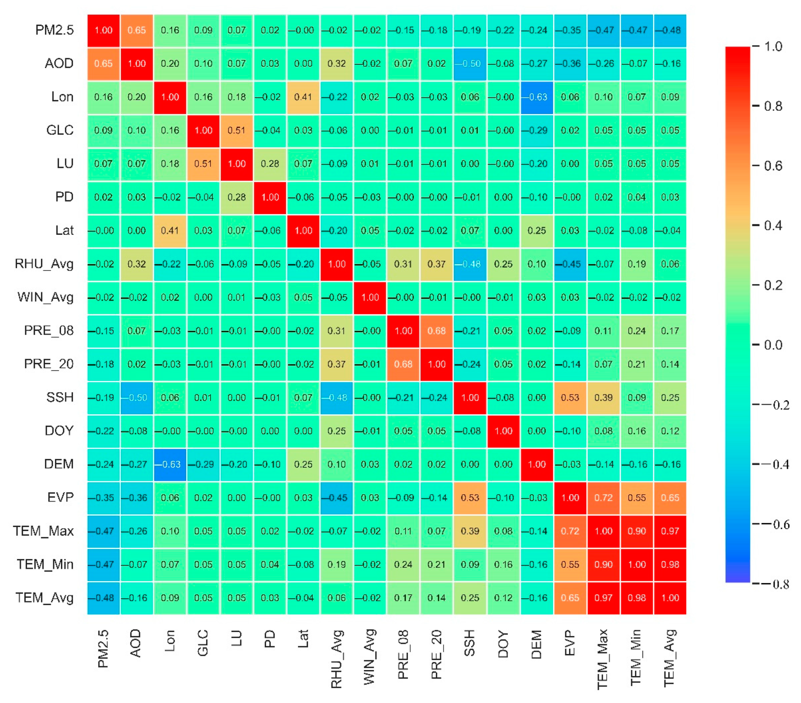
| Positive Variables | Negative Variables | ||||||
|---|---|---|---|---|---|---|---|
| NO. | Variable | r | p_Value | NO. | Variable | r | p_Value |
| 1 | AOD | 0.65 | 0.00 | 1 | TEM_Avg | −0.48 | 0.00 |
| 2 | Lon | 0.16 | 0.00 | 2 | TEM_Min | −0.47 | 0.00 |
| 3 | GLC | 0.09 | 0.00 | 3 | TEM_Max | −0.47 | 0.00 |
| 4 | LU | 0.07 | 0.00 | 4 | EVP | −0.35 | 0.00 |
| 5 | PD | 0.02 | 0.00 | 5 | DEM | −0.24 | 0.00 |
| 6 | DOY | −0.22 | 0.00 | ||||
| 7 | SSH | −0.19 | 0.00 | ||||
| 8 | PRE_20 | −0.18 | 0.00 | ||||
| 9 | PRE_08 | −0.15 | 0.00 | ||||
| 10 | WIN_Avg | −0.02 | 0.00 | ||||
| 11 | RHU_Avg | −0.02 | 0.00 | ||||
| 12 | Lat | −0.00 | 0.26 | ||||
| Model | Study Area | Model Validation | Predictive Power | References Origin | |||||
|---|---|---|---|---|---|---|---|---|---|
| R2 | RMSE | MAE | MPE | Slope | Intercept | Daily R2 | |||
| RF | Texas | 0.69–0.81 | - | - | - | - | - | - | [54] |
| MEM | Texas | 0.62–0.74 | - | - | - | - | - | - | [54] |
| MLR | Texas | 0.45–0.59 | - | - | - | - | - | - | [54] |
| MLR | Eastern United States | 0.75 | - | - | - | 0.89 | - | - | [55] |
| STR | Henan-Hubei-Hunan | 0.59 | 29.43 | - | 19.88 | 0.62 | 25.55 | - | [49] |
| GAM | Beijing-Tianjin-Hebei | 0.8 | 23 | - | - | 0.92 | 5.8 | - | [60] |
| GWR | Beijing-Tianjin-Hebei | 0.81 | 22 | - | - | 0.99 | 8.18 | - | [60] |
| Mixed model | Beijing-Tianjin-Hebei | 0.87 | 19 | - | - | 0.9 | 7 | - | [60] |
| RF | Tehran | 0.68 | 17.52 | - | - | - | - | - | [52] |
| DNN | New York State | 0.66 | 2.18 | - | 1.58 | - | - | - | [56] |
| RF | New York State | 0.81 | 1.63 | - | 1.15 | - | - | - | [56] |
| GBM | New York State | 0.85 | 1.44 | - | 1.02 | - | - | - | [56] |
| Ensemble model | New York State | 0.86 | 1.43 | - | 1 | - | - | - | [56] |
| Statics model | Northeastern USA | 0.88 | 2.32 | - | - | 1.01 | - | - | [57] |
| Ensemble model | United States | 0.86 | 2.79 | - | - | 0.96 | - | - | [58] |
| RF | Iraq and Kuwait | 0.71 | - | - | - | - | - | - | [14] |
| GA-SVM | Shaanxi | 0.84 | 12.1 | 10.07 | - | - | - | - | [51] |
| XGBoost | New England states | 0.64–0.80 | 2.91–4.42 | - | - | - | - | - | [59] |
| RF | South Africa | 0.8 | 9.4 | - | - | 1.13 | −3.66 | - | [15] |
| XGBoost | Tehran | 0.74 | 8.97 | 6.88 | - | - | - | - | [53] |
| Extra Trees | Tehran | 0.68 | 9.63 | 7.66 | - | - | - | - | [53] |
| Random Forest | Tehran | 0.69 | 9.51 | 7.5 | - | - | - | - | [53] |
| SVR | Tehran | 0.63 | 10.36 | 7.98 | - | - | - | - | [53] |
| DBN | Tehran | 0.66 | 9.99 | 7.67 | - | - | - | - | [53] |
| DAE + SVR | Tehran | 0.68 | 9.75 | 7.32 | - | - | - | - | [53] |
| MLR | China | 0.41 | 20.04 | 30.03 | - | 0.41 | 30.03 | 0.38 | [25] |
| GWR | China | 0.53 | 23.28 | 19.26 | - | 0.61 | 20.93 | 0.44 | [25] |
| Two-stage | China | 0.71 | 18.59 | 14.54 | - | 0.71 | 15.1 | 0.35 | [25] |
| RF | China | 0.81 | 17.91 | 11.5 | - | 0.77 | 12.56 | 0.53 | [25] |
| STRF | China | 0.85 | 15.57 | 9.77 | - | 0.82 | 9.64 | 0.55 | [25] |
| STEM | China | 0.89 | 10.35 | 6.71 | - | 0.86 | 6.16 | 0.65 | [25] |
| GBDT | China | 0.92 | 10.14 | 6.02 | - | 0.92 | 3.73 | - | [48] |
| RF | Guangdong | 0.80–0.83 | 8.20–9.20 | - | - | 0.76–0.78 | - | - | [50] |
| RF | Shenzhen | 0.88 | 4.34 | - | - | 0.77 | 8.43 | - | [27] |
| IRF | Shenzhen | 0.92 | 3.66 | - | - | 0.82 | 6.6 | - | [27] |
| XGBoost | GUA | 0.91 | 11.58 | 7.75 | - | 0.87 | 6.81 | - | Our study |
| RF-XGBoost | GUA | 0.93 | 12.49 | 8.42 | - | 0.9 | 5.42 | 0.61 | Our study |
| Model | Out-of-Sample Test | TC | MC | Model-Prediction | ||||||
|---|---|---|---|---|---|---|---|---|---|---|
| Samples | R2 | RMSE | MAE | (s) | (MB) | Samples | R2 | RMSE | MAE | |
| RF | 12,368 | 0.88 | 13.36 | 8.28 | 16.00 | 354.71 | 2765 | 0.52 | 25.50 | 19.17 |
| ERT | 0.90 | 11.93 | 7.54 | 6.00 | 489.78 | 0.57 | 24.14 | 18.03 | ||
| GBDT | 0.84 | 15.27 | 10.10 | 6.00 | 152.41 | 0.48 | 26.67 | 19.33 | ||
| XGBoost | 0.89 | 12.56 | 7.94 | 1.00 | 169.02 | 0.40 | 28.63 | 19.72 | ||
| LightGBM | 0.90 | 12.23 | 7.81 | 0.00 | 169.64 | 0.40 | 28.60 | 19.92 | ||
| RF-XGBoost | 34,956 | 0.92 | 12.85 | 8.73 | 40.00 | 2281.53 | 13,493 | 0.54 | 24.76 | 18.64 |
Publisher’s Note: MDPI stays neutral with regard to jurisdictional claims in published maps and institutional affiliations. |
© 2022 by the authors. Licensee MDPI, Basel, Switzerland. This article is an open access article distributed under the terms and conditions of the Creative Commons Attribution (CC BY) license (https://creativecommons.org/licenses/by/4.0/).
Share and Cite
Lin, L.; Liang, Y.; Liu, L.; Zhang, Y.; Xie, D.; Yin, F.; Ashraf, T. Estimating PM2.5 Concentrations Using the Machine Learning RF-XGBoost Model in Guanzhong Urban Agglomeration, China. Remote Sens. 2022, 14, 5239. https://doi.org/10.3390/rs14205239
Lin L, Liang Y, Liu L, Zhang Y, Xie D, Yin F, Ashraf T. Estimating PM2.5 Concentrations Using the Machine Learning RF-XGBoost Model in Guanzhong Urban Agglomeration, China. Remote Sensing. 2022; 14(20):5239. https://doi.org/10.3390/rs14205239
Chicago/Turabian StyleLin, Lujun, Yongchun Liang, Lei Liu, Yang Zhang, Danni Xie, Fang Yin, and Tariq Ashraf. 2022. "Estimating PM2.5 Concentrations Using the Machine Learning RF-XGBoost Model in Guanzhong Urban Agglomeration, China" Remote Sensing 14, no. 20: 5239. https://doi.org/10.3390/rs14205239