Evaluating Optical Remote Sensing Methods for Estimating Leaf Area Index for Corn and Soybean

Abstract

The leaf area index (LAI) is a key crop biophysical variable influencing many vegetation processes. Spatial LAI estimates are essential to develop and improve spatial modeling tools to monitor vegetation conditions at large regional scales. Numerous optical remote sensing methods have been explored to retrieve crop-specific LAI at a regional scale using satellite observations. However, a major challenge is selecting a method that performance well under various conditions without local scale calibration. As such, we assessed the performance of existing statistical and physical approaches, developed based on parametric, non-parametric and radiative transfer model (RTM)-look-up-table based inversion, using field observations from two geographically distant locations and Landsat 5, 7, and 8 satellite observations. These methods were implemented for corn and soybeans cultivated at two locations in the U.S (i.e., Mead, Nebraska, and Bushland, Texas). The evaluation metrics (i.e., Root Mean Square Error (RMSE), Mean Absolute Error (MAE), and Coefficient of Determination (R²)) were used to study the performance of each method, and then the methods were ranked based on these metrics. Our study showed that overall parametric methods outperformed other methods. The RMSE (MAE) for the top five methods was less than 1.3 (0.95) for corn and 1.0 (0.8) for soybeans, irrespective of location. Even though they outperformed, parametric methods exhibited inconsistency in their performance. For instance, the SR_CA_cross method ranked 1 for corn, however, it performed poorly for soybean (ranked 15). The non-parametric methods showed moderate accuracy partly due to the availability of a smaller number of observations for training. The RTM-LUT inversion physical-based approach was found to perform reasonably well RMSE (MAE) less than 1.5 (1.0) consistently irrespective of location and crop, implying that this approach is more suitable for regional-scale LAI estimation. The results of this study highlighted the drawbacks and advantages of available optical remote sensing approaches to estimate LAI for corn and soybean crops using Landsat imagery. These results are of interest for remote sensing and modeling communities developing spatial-scale approaches to model and monitor agricultural vegetation.

1. Introduction

Leaf area index (LAI), the total one-sided area of leaves per unit area of land, is a fundamental crop parameter that determines the absorption rate of photosynthetic active radiation (PAR) [1,2,3,4]. LAI also affects the exchange of water vapor, and near-surface climate through influencing albedo [5,6]. Thus, LAI has been used to describe crop growth, water use, carbon assimilation, and near surface climate variables. LAI is an essential intermediate state variable in process-based crop models and has considerable influence on the simulation of other processes such as evapotranspiration and crop potential biomass [7,8,9,10].

Given that, LAI is strongly related to important plant biophysical processes, spatial scale LAI estimates are essential for assessing crop conditions and potential yields at regional to global scales [11]. Regional LAI estimates can be used in combination with other descriptors and in process-based crop models to develop operational spatial crop monitoring and forecasting tools. For instance, energy balance models (e.g., DisALEXI) require LAI as an input for computing soil/canopy partitioning, and spatial LAI estimates have been used to implement energy balance models at large spatial scales to produce regional estimates of evapotranspiration [12].

Optical remote sensing observations have been widely explored to retrieve LAI at various spatial scales ranging from field to global scale since they are cost-effective and enable the acquiring of periodical observations in a timely manner [13,14,15]. There are primarily two optical remote sensing approaches used for LAI estimation: (1) statistical-based empirical approaches, and (2) radiative transfer model (RTM) based physical approaches. Statistical-based approaches commonly rely on simple linear, polynomial, exponential, or logarithmic models that relate field scale LAI measurements with spectral data [16,17,18,19]. To maximize the signal-to-noise ratio, various mathematical transformations have been used in the development of parametric models to estimate LAI. The vegetative indices, mathematical combination of two or more spectral bands, are most commonly used in the parametric models, and some other transformations include bandwidth analysis and red edge inflection point [16,20,21,22,23,24,25,26]. In addition, some studies have explored nonparametric regression methods such as principal component analysis, partial least square regression and neural networks [27,28,29,30]. The empirical models have been widely used, as they are relatively simple, computationally efficient, and easy to implement at large spatial scale. However, these models are often non-transferable to other sites characterized with different environmental conditions or to other spectral data from different imagery. Further, the performance of statistical models depends on quality and size of the in-situ data, and it is often challenging to acquire robust and high-quality in-situ data to develop statistically sound empirical models.

Physically based approaches are developed based on the radiative transfer models (RTMs). The RTMs are built on physical principles of photon transport through vegetation, and simulate canopy reflectance using leaf biophysical characteristics, soil background, and viewing and illumination geometry [31,32,33,34,35]. Since these approaches rely on the vegetation biophysical and biochemical properties, in situ data is not required, and these models are found to be adapted to various conditions. However, their retrieval performance varies widely based on specified input parameters (e.g., leaf angle distribution, soil background reflectance), and inversion approach. For instance, the MOD15 LAI algorithm uses broad crop (e.g., broadleaf crops) categories to parametrize the 3D radiative transfer model [36]. As such, MOD15 LAI tends to underperform when compared with measured crop-specific LAI on agricultural sites [37]. There are typically three types of inversion approaches including Look-Up Tables (LUT), machine learning algorithms (e.g., Neural Networks, Support Vector Machine) and iterative optimization [38,39,40,41,42,43]. Each of these inversion approaches has tradeoffs. For example, LUT approaches are simple to execute, and may yield better LAI estimates but are computationally very intensive, while machine learning algorithms are relatively efficient but may compromise the accuracy of LAI estimates. These approaches are usually ill-posed, which means a numerical solution may not result in stable and accurate inversion performance [38,44].

To take advantage of both statistical and physically based approaches, a hybrid approach has been introduced [45,46]. Regression models for LAI estimation using the calibration of RTMs were developed [16]. Unlike in the statistical approaches where spectral imagery-based vegetative indices and in-situ LAI measurements are used to develop predictive equations, hybrid approaches use simulated canopy reflectance by RTM under a range of LAI values, and develop predictive models using simulated reflectance-based vegetative indices and LAI values used to simulate canopy reflectance. Since these approaches are independent of in-situ observations, they are expected to perform well irrespective of location. However, a misrepresentation of model parameters often leads to uncertainties in RTM simulations, which in turn may have negative impacts on the performance of hybrid approaches.

There are several review research studies on LAI estimation using remote sensing [47,48,49,50,51,52]. These studies show the importance, limitations, and strategies to improve the accuracy of each of these methods [49,53,54,55]. Most of these studies focused on forest cover, and very few reviewed the existing LAI estimation methods for cropland using optical remote sensing including multispectral, hyperspectral and LiDAR [47,52]. All of the existing studies focused on reviewing existing studies and underscoring the advantages and limitations of current approaches. For example, Liu [52] highlighted the technical issues such as the curse of dimensionality and ill-posed problems in hyperspectral remote sensing-based crop LAI estimation. None of these review studies compared different methods of LAI estimation using field observations and satellite remote sensing data.

Considering the presence of various options for LAI estimation and respective advantages and limitations, it is important to assess their performance under various geographical conditions, different cropping systems and with different spectral data. Even though there are many optical methods that exist, the major challenge is to select an appropriate approach that performs well when implementing large regional scales using satellite imagery. Local calibration of a particular LAI method may not help improve the prediction skill when implemented at large regional scale since considerable differences in climate, soil, and geographical conditions are expected. Further, the research that provides the transferability of existing methods of LAI estimation for different crops is not present. Therefore, the overall objective of this study is to assess the performance of available optical remote sensing approaches, without calibration to local conditions, to estimate LAI for corn and soybean cultivated under different geographical and management conditions using satellite imagery. We choose corn and soybeans in this study because they are major cropping systems in the U.S and worldwide. Further, we selected two geographically distant locations in the U.S: Mead, NE and Bushland, TX, and used Landsat five, seven, and eight satellite observations, and evaluated different empirical (i.e., parametric linear or exponential regression models and non-parametric machine learning algorithms) and physical based approaches (LUT-based inversion, and hybrid RTM-empirical) to estimate LAI of irrigated and non-irrigated corn and soybeans cultivated at these locations.

2. Data Used

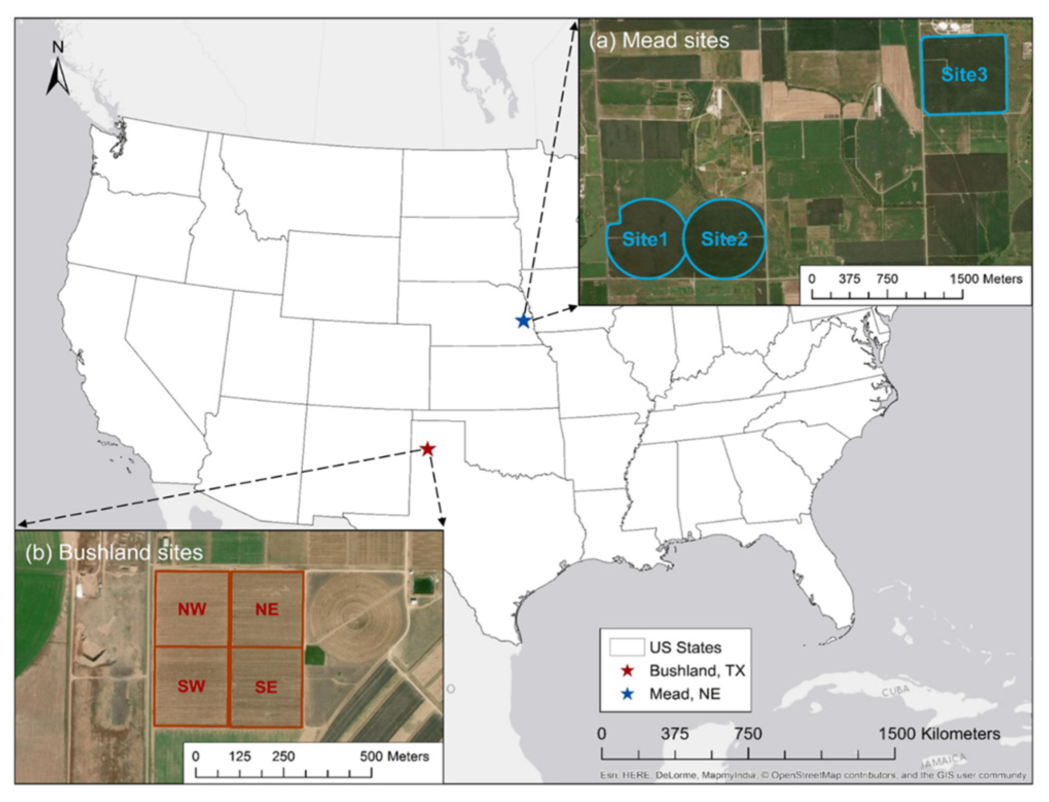
2.1. Study Sites and Field Observations

Field measurements of LAI collected from three AmeriFlux sites near Mead, Nebraska (NE) and four lysimeter field sites in Bushland, Texas (TX) were used in this study to assess the performance of LAI models and to quantify their transferability (Figure 1).

The three field sites near Mead, NE have been maintained by the University of Nebraska–Lincoln as part of the AmeriFlux network (https://ameriflux.lbl.gov/, accessed on 10 March 2022) ever since 2001 (Figure 1a). Having a humid continental climate, these Mead sites stay humid throughout the year without dry seasons, although winters are severe and summers are hot. The mean annual temperature at these sites is 10.07 °C and the mean annual precipitation is 790.37 mm (https://ameriflux.lbl.gov/sites/siteinfo/US-Ne1, accessed on 1 September 2022). The soils are deep silty clay loam consisting of Tomek, Yutan, Filbert, and Filmore soil series. Irrigated with a center pivot system, the Mead sites have been planted with corn-soybean rotation for ten years under no-till, prior to the data collection at 2001. The field sites were tilled just before 2001 planting and applied with phosphorus and potassium fertilizers including the leftover residues. After each harvest, a nitrogen fertilizer is mixed on the residue. From 2001 to 2016, both Sites 2 and 3 continued with corn-soybean rotation, while only corn was planted in Site1 (

Table 1. Years and sites of corn and soybean growing at the AmeriFlux sites, Mead, NE between 2001 and 2016.

Year	Site 1	Site 2	Site 3
2001	Corn	Corn	Corn
2002	Corn	Soybean	Soybean
2003	Corn	Corn	Corn
2004	Corn	Soybean	Soybean
2005	Corn	Corn	Corn
2006	Corn	Soybean	Soybean
2007	Corn	Corn	Corn
2008	Corn	Soybean	Soybean
2009	Corn	Corn	Corn
2010	Corn	Corn	Soybean
2011	Corn	Corn	Corn
2012	Corn	Corn	Soybean
2013	Corn	Corn	Corn
2014	Corn	Soybean	Soybean
2015	Corn	Corn	Corn
2016	Corn	Soybean	Soybean

). In addition, Sites 1 and 2 are consistently irrigated, while Site 3 is rainfed. At all three sites, green LAI measurements were taken using a leaf area meter (Model LI-3100, Li-Cor).

The research field (about 0.2 km² in total) near Bushland, TX is located at the Conservation and Production Research Laboratory (CPRL) of the USDA Agricultural Research Service (Figure 1b). This field is further separated into four square field sites identified as NE, SE, NW, and SW, with a weighting lysimeter set up in the center of each field. Different from the humid Mead sites, the Bushland sites have a semi-arid temperate climate with large diurnal and daily variability of temperature [56]. The Pullman clay loam (a fine, mixed, superactive, thermic Torrertic Paleustoll) is the major soil type in the study sites. We obtained green LAI observations collected, using the electronic leaf area meter (Delta-T Devices Ltd., Cambridge, UK), from 1995 to 2010 for the four sites in this study. Corn, soybean, cotton, winter wheat, sorghum, and sunflower were planted during the entire data collection period with rotations. Specifically, we focused on the sites and years in which corn and soybean were grown as listed in

Table 2. Years and sites of corn and soybean growing at the USDA Lysimeter sites, Bushland, TX between 1995 and 2010.

Year	NE	SE	NW	SW
1995	-	-	Irrigated soybean	Irrigated soybean
2003	Irrigated soybean	Irrigated soybean	-	-
2004	Irrigated soybean	Irrigated soybean	-	-
2006	Irrigated corn	-	-	-
2007	-	Irrigated corn	-	-
2010	-	-	Dryland soybean	Dryland soybean

for assessment.

2.2. Remote Sensing Datasets

Landsat 5 Thematic Mapper (TM), Landsat 7 Enhanced Thematic Mapper Plus (ETM+), and Landsat 8 Operational Land Imager (OLI) data were used to estimate crop LAI in this study for both Bushland and Mead sites. We collected Level-2 Surface Reflectance products generated through Landsat Ecosystem Disturbance Adaptive Processing System (LEDAPS) [57] and Landsat Surface Reflectance Code (LaSRC) [58] systems distributed by U.S. Geological Service (USGS). All available Landsat tiles covering the field sites during the years of field data collection were downloaded. The details were summarized in

Table 3. Summary of Landsat Level-2 surface reflectance data used in this study.

Sites	Spatial Resolution	Sensors	WRS2 Tiles
Mead, NE	30 m	Landsat 5 TM, Landsat 7 ETM+, Landsat 8 OLI	Path 28 Row 31
Bushland, TX	30 m	Landsat 5 TM, Landsat 7 ETM+	Path 30 Row 36, Path 31 Row 35, Path 31 Row 36

.

2.3. Landsat Data Preparation

For both Mead and Bushland sites, we predefined a processing region of 1000 × 1000 30-m pixels (9 km²) centered at the field sites for Landsat data. Prior to LAI modeling, we first masked out the cloud and cloud shadow pixels based on the Quality Assessment (QA) band provided by the Level-2 product. We then adopted a gap-filling algorithm [59] developed for Landsat time series data to fill the scan-line corrector (SLC) gaps in ETM+ data acquired after 2003 and the masked cloud/shadow pixels for all Landsat imagery.

We further applied the locally estimated scatterplot smoothing (LOESS) algorithm to reduce the impacts of temporal gaps and noises on time series Landsat data. We extracted the yearly time series values of each surface reflectance and spectral index for each field plot separately. For each year and each field plot, we used the LOESS algorithm with a smoothing factor of 0.25 for fitting each surface reflectance and index by day of the year. The smoothed data were then used to estimate LAI values with different types of methods as described in Section 3 below.

3. Crop LAI Estimation Methods

We summarized the commonly used LAI retrieval methods into two broad categories for transferability assessment based on the literature review in this manuscript: (1) empirical models and (2) physical-based models. The first category refers to the empirical models developed using field observations as the training data, while models within the second category are derived from simulated datasets generated from canopy radiative transfer models such as PROSAIL [60,61]. The empirical models were further categorized into (1) parametric equations such as linear or exponential regression models, and (2) non-parametric models developed from machine learning algorithms. We considered three types of physical-based approaches categorized based on LAI retrieval strategies: (1) RTM-parametric modeling, (2) RTM-non-parametric modeling and (3) RTM-LUT-based inversion. The methods evaluated in this study and the workflow of the assessment were summarized in Figure 2.

3.1. Empirical Modeling Methods

3.1.1. Parametric Equations

Estimating LAI values based on their empirical relationships with spectral vegetation indices has been the most widely used method for large-scale LAI retrieval with optical remote sensing data, due to its computational efficiency and easiness [18,62]. Most vegetation indices (VIs) utilized in LAI retrieval are derived from surface reflectance of near-infrared (NIR) and red bands, such as the Normalized Difference Vegetation Index (NDVI), Enhanced Vegetation Index (EVI), and Green Atmospherically Resistant Vegetation Index (GARVI) [62]. Hyperspectral indices have also been frequently utilized to estimate the LAI of different crop types in precision agriculture practices [52]. Although they are often found to result in LAI estimates with higher accuracy due to their finer spectral resolutions, their applications in monitoring the spatial-temporal distribution of LAI are largely limited by hyperspectral data availability.

We reviewed existing literature that documented parametric empirical methods (Table S1) developed based on various VIs (

Table 4. Details of vegetation indices used in empirical parametric equations.

Index	Formula	References
NDVI	$\frac{{\rho }_{NIR}-{\rho }_{Red}}{{\rho }_{NIR}+{\rho }_{Red}}$	[64]
gNDVI	$\frac{{\rho }_{NIR}-{\rho }_{Green}}{{\rho }_{NIR}+{\rho }_{Green}}$	[65]
SR	$\frac{{\rho }_{NIR}}{{\rho }_{Red}}$	[66]
RSR	$\frac{{\rho }_{NIR}}{{\rho }_{Red}}\times (1-\frac{{\rho }_{SWIR}-{\rho }_{SWIRmin}}{{\rho }_{SWIRmax}-{\rho }_{SWIRmin}})$	[67]
EVI	$\frac{2.5\times \left({\rho }_{NIR}-{\rho }_{Red}\right)}{{\rho }_{NIR}+6\times {\rho }_{Red}-7.5\times {\rho }_{Blue}+1}$	[68]
GARVI	$\frac{{\rho }_{NIR}-\left[{\rho }_{Green}-\left({\rho }_{Blue}-{\rho }_{Red}\right)\right]}{{\rho }_{NIR}+\left[{\rho }_{Green}-\left({\rho }_{Blue}-{\rho }_{Red}\right)\right]}$	[65]
WDRVI	$\frac{\alpha \times {\rho }_{NIR}-{\rho }_{Red}}{\alpha \times {\rho }_{NIR}+{\rho }_{Red}}$	[63]
gWDRVI	$\frac{\alpha \times {\rho }_{NIR}-{\rho }_{Green}}{\alpha \times {\rho }_{NIR}+{\rho }_{Green}}+\frac{1-\alpha }{1+\alpha }$	[63]
Clgreen	$\frac{{\rho }_{NIR}}{{\rho }_{Green}}-1$	[69]

) and selected those that provide empirical equations for LAI estimation for individual crops or crops in general from highly cited literature. The VIs used here are NDVI, green NDVI (gNDVI), Simple Ratio (SR), Reduced SR (RSR), EVI, GARVI, Wide Dynamic Range Vegetation Index (WDRVI), green WDRVI (gWDRVI), and Green Chlorophyll Index (Cl_green). If available, we used more than one empirical equation developed using a specific vegetative index for estimating LAI for a given crop. Since Viña et al. [62] did not explicitly mention the value of the weighting coefficient α used in their manuscript, we used both 0.1 and 0.2 as α as to calculate WDRVI and to model LAI with the corresponding equation in this study (identified as WDRVI_Ne1_Viña and WDRVI_Ne2_Viña respectively), considering the range of 0.1–0.2 for α [63]. After identifying the equations to use, we then calculated each VI and applied the selected equations to estimate LAI values for crops cultivated at both Bushland and Mead sites. For the years with field observations, we retrieved LAI values using Landsat data for the entire year.

3.1.2. Non-Parametric Models

Existing studies have demonstrated the effectiveness of non-parametric models in estimating LAI from optical spectral information using machine learning algorithms [70,71,72]. Specifically, Neural Networks (NN), Random Forest (RF), and Support Vector Machine (SVM) are among the most commonly applied methods. Different from parametric equations, these models are not developed under assumptions of input variable distribution or autocorrelation [73].

We followed the model settings based on existing literature as listed in

Table 5. Pure empirical non-parametric models used in this study.

Models	Sites	Crop Types	Settings	References
SVM	Italy, Austria	Multiple types	Linear kernel function, least square	[74]
NN	Northeastern China	Corn	Back-propagation algorithm for minimizing misfit function	[75]
RF	Italy, Austria	Multiple types	Number of trees = 500 Number of input var at each split = 2	[74]

. Since there are no available explicit formats of these models, we trained them using in-situ data collected at Mead sites and validated the models with field data from the Bushland sites. Surface reflectance from all eight bands of Landsat was used as input parameters for model training and validation. As in both sites, LAI data are only available for corn and soybean, we simply assessed the transferability of non-parametric methods for these two crop types.

3.2. Physical-Based Methods

We examined the aforementioned retrieval methods derived based on a simulated dataset from RTMs. For parametric equations extracted with physical-based models, we extracted existing equations from the literature to assess their performance and stability in retrieving LAI values at different regions. Different from parametric equations, neither non-parametric models nor LUT-inversion output are explicitly available from existing literature. We then derived simulated datasets with the coupling of the PROSPECT and SAIL model, also known as PROSAIL [41], to evaluate the performance of non-parametric models and the LUT-inversion method at both field sites. Coupling a leaf optical properties model PROSPECT and a canopy bidirectional reflectance model SAIL (Scattering by Arbitrary Inclined Leaves), PROSAIL has the capability to physically describe the spectral and direction properties of vegetation canopy in terms of leaf biochemistry characteristics and canopy architecture [61]. It has been widely utilized in retrieving the bidirectional surface reflectance spectrum of multiple crop types for effective estimation of crop LAI [43,76,77,78]. Thus, in this manuscript, we adopted the PROSAIL model to generate simulated LUTs for training non-parametric models and LUT-based inversion methods.

We first generated crop canopy realizations for each crop type involved in this study using LUTs with 100,000 cases of canopy variable combination as suggested by Richter et al. [77]. We defined the range and distribution of the major parameters for PROSPECT and SAILH models to establish the LUTs based on previous studies (

Table 6. Parametric settings for the PROSAIL model in this study.

Model	Parameters	Abbr.	Units	Ranges	Distribution
PROSPECT	Leaf structure index	N	Unitless	1–2.5	Uniform
	Leaf chlorophyll content	Cab	μg/cm2	10–80	Gaussian (μ:45, σ:20)
	Leaf dry matter content	Cm	g/cm2	0.001–0.03	Uniform
	Leaf water content	Cw	cm	0.002–0.05	Uniform
	Brown pigments content	Cbp	Unitless	0–2	Uniform
	Leaf carotenoid content	Car	μg/cm2	0–16	Uniform
SAILH	Leaf area index	LAI	m2/m2	0.1–7	Gaussian
	Hot spot parameter	SL	Unitless	0.05–1	Uniform
	Soil reflectance factor	ρS	Unitless	0–1	Uniform
	Solar zenith angle	θS	Degree	Based on Landsat data acquisition conditions

). Parameters describing the solar and sensor positions in the SAILH model, including solar zenith angle, view zenith angle, and solar-sensor azimuth angle, were determined separately for Mead and Bushland sites based on the metadata file for the corresponding Landsat tiles.

3.2.1. Physical-Based Parametric Equations

Different from purely empirical equations, physical-based parametric models have been developed with VIs computed using simulated reflectance based on RTMs such as PROSAIL to estimate crop LAI in different regions [43,79,80]. Similar to Section 3.1.1, we identified a list of empirical equations (Table S2) developed based on PROSAIL with a variety of spectral indices (

Table 7. Details of additional vegetation indices used in physical-based parametric equations.

Index	Formula	References
RDVI	$\frac{{\rho }_{NIR}-{\rho }_{Red}}{\sqrt{{\rho }_{NIR}+{\rho }_{Red}}}$	[81]
OSAVI	$\left(1+0.16\right)\times \frac{{\rho }_{NIR}-{\rho }_{Red}}{{\rho }_{NIR}+{\rho }_{Red}+0.16}$	[82]
MSAVI	$\frac{1}{2}\times \left[2\times {\rho }_{NIR}+1-\sqrt{{\left(2\times {\rho }_{NIR}+1\right)}^2-8\times \left({\rho }_{NIR}-{\rho }_{Red}\right)}\right]$	[83]
MTVI1	$1.2\times \left[1.2\times \left({\rho }_{NIR}-{\rho }_{Green}\right)-2.5\times \left({\rho }_{Red}-{\rho }_{Green}\right)\right]$	[79]
MTVI2	$\frac{1.5\times \left[1.2\times \left({\rho }_{NIR}-{\rho }_{Green}\right)-2.5\times \left({\rho }_{Red}-{\rho }_{Green}\right)\right]}{\sqrt{{\left(2\times {\rho }_{NIR}+1\right)}^2-\left(6\times {\rho }_{NIR}-5\times \sqrt{{\rho }_{Red}}\right)-0.5}}$	[79]
SPVI	$0.4\times 3.7\times \left({\rho }_{NIR}-{\rho }_{Red}\right)-1.2\times \left|{\rho }_{Red}-{\rho }_{Green}\right|$	[84]

) for crop LAI retrieval from existing literature. These VIs are Renormalized Difference Vegetation Index (RDVI), Optimized Soil Adjusted Vegetation Index (OSAVI), Modified Soil Adjusted Vegetation Index (MSAVI), Modified Triangular Vegetation Index (MTVI), and Spectral Polygon Vegetation Index (SPVI). Since the formulas of these developed models are explicitly available, we calculated each of the indices and then applied them to retrieve LAI with Landsat data for transferability assessment.

3.2.2. Physical-Based Non-Parametric Models

Non-parametric models such as SVM, NN and RF have also been integrated with physical-based models for LAI retrieval [70,75,85,86,87]. Simulated datasets generated from RTMs such as PROSAIL function as the data source for non-parametric model training. We explored commonly used machine learning algorithms (i.e., NN, RF, and SVM) to train the physical-based models for mead sites. We followed the same settings of the three algorithms as we used in Section 3.1.2. Then we implemented trained models over Bushland sites using Landsat surface reflectance data to assess their performance. The performance was evaluated using in-situ data at Bushland.

3.2.3. LUT-Based Inversion

The same simulated dataset generated by the PROSAIL model in Section 3.2.2 was used for the LUT-based inversion method. For each pixel, we applied a widely used cost function that calculates the root mean square error (RMSE) of all surface reflectance bands between the measured and the LUT values [77,88,89] to estimate the LAI values based on the corresponding LUT. The cost function is defined using the following equation:

$$\mathrm{RMSE}=\sqrt{\frac{1}{n_{\lambda }}{\displaystyle \sum }_{i=1}^{n_{\lambda }}{\left({\rho }_{measure}^i-{\rho }_{LUT}^i\right)}^2}$$

(1)

We then calculated the RMSE value for each combination in the LUT for each pixel. To avoid the ill-posed issue in the inversion of RTMs, we determined the final LAI value for a certain pixel by averaging all the LAI values with 10% of the smallest RMSE value in the last step.

3.3. Accuracy Assessment

After retrieving LAI values for both Mead and Bushland sites using the methods described above, we further assessed their accuracy through assessing their performance at each site using statistical metrics. Many metrics for assessing the accuracy of a predictive models have been studied and used [90,91,92] and Root Mean Squared Error (RMSE), Mean Absolute Error (MAE), and R-squared (R²) are the most common among them. Therefore, these three commonly used statistical metrics are considered in this study. The R² is the relative metric that measures the variation between predicted and observed datasets, where, RMSE and MAE present the error components [93]. RMSE, MAE, and R² were computed using observed and estimated LAI values using models. The models were then ranked based on the weighted average of these evaluation metrics. Since RMSE and MAE consider differences in predicted and observed values and quantify the error, they were given more weights (0.4 for each one) compared to R² (0.2 weight) as it is a relative metric. Since Mead and Bushland sites represent different irrigation and climate conditions, we calculated three metrics at each site separately to assess the performance of each method at both sites. Further, the performance of each method was examined based on crop type, irrigation practices, and study locations.

4. Results

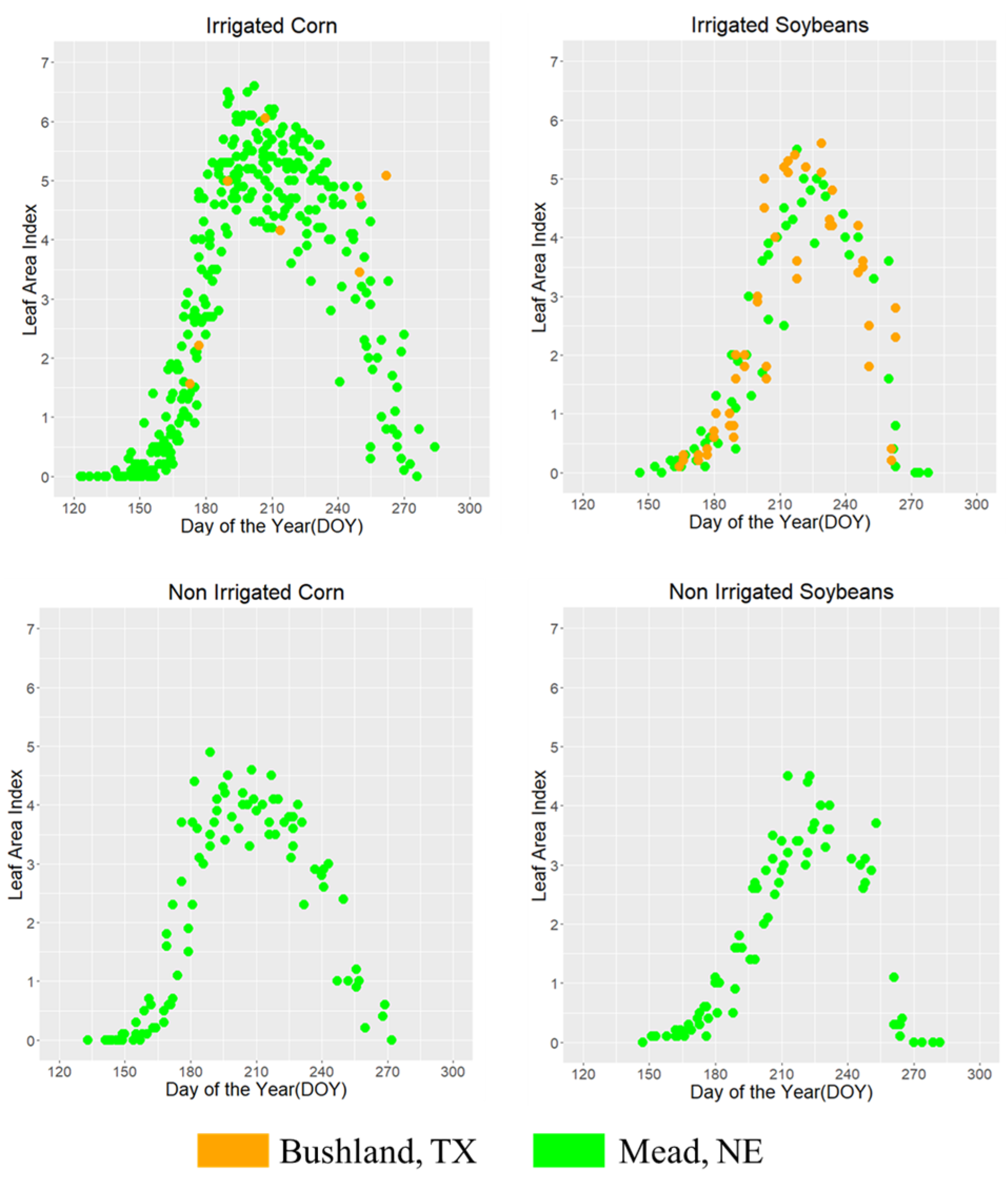
4.1. Variability in LAI Observations

Field observations used in this study showed considerable variation in LAI values, reflecting changes in crop type and irrigation practices (Figure 3). Irrespective of location, corn LAI values were higher with maximum LAI values ranging from 5–7 depending on location and irrigation management. Soybean maximum LAI values ranged from 4.5–5.6, approximately 15% lower than corn. Under irrigation practice, LAI values were about 23% higher compared to non-irrigation practices. Bushland LAI values were slightly higher even though values were not significant at the p < 0.05 level. This was against our expectations because the growing conditions are drier in Bushland expecting lower LAI values compared to the Mead site. This slight discrepancy could be attributed to measurement errors, which may influence the performance of LAI retrieval methods.

4.2. Empirical Approaches

Total of seventeen empirical parametric methods for LAI estimation were evaluated which are based on nine vegetation indices as listed in Table 4 and for different locations. Most of the studied methods performed, irrespective of the location, reasonably well for both corn and soybean with R² values greater than 0.80. Similarly, more than 85% of methods resulted in estimates with RMSE values less than 2 with average RMSE values of 1.73 and 1.56 for corn and soybean, respectively. However, the performance varies considerably among the methods depending on various factors such as location, crop type, and spectral bands used in the development of methods.

For instance, overall, when considering both corn and soybean LAI estimates, methods performed slightly better at Mead sites (average RMSE = 1.60 and MAE = 1.25) than at Bushland sites (average RMSE = 1.69 and MAE = 1.32). This could be partly because of possible discrepancies in LAI observations at Bushland sites. The average RMSE (MAE) values for corn and soybeans LAI estimates at Mead sites were 1.63 (1.28) and 1.56 (1.22), respectively, while at Bushland sites, the average RMSE (MAE) values were 1.83 (1.39) and 1.55 (1.25) for corn and soybeans, respectively. These results indicated that methods outperformed for corn at Mead sites, and for soybeans, a significant difference was not noticed in the performance. Overall, the empirical parametric methods achieved top five ranks (i.e., WDRVI_Ne2_Viña, gWDRVI_Ne_NR, SR_Ne_NR, Clgreen_Ne_NR, and SR_CA_Kross) for corn at Mead site (Table S4) whereas only one method is in the top five ranks (i.e., SR_CA_Kross) at Bushland site. The lower performance of parametric methods for corn at Bushland could be attributed to the lower number of LAI observations for corn. These methods secured all five top ranks for soybeans at the Bushland site (Table S5). The better performance for soybean at Bushland in part, could be due to a higher number of LAI observations.

Three non-parametric approaches SVM, NN, and RF showed moderate accuracy and the average RMSE (MAE) was 1.60 (1.25) and 1.31 (1.07) for corn and soybeans, respectively. The average R² was ~0.83 for both crops with considerably low variation depending on the methods and the locations. The methods were found somewhat more accurate for soybeans. Overall, SVM was ranked three, and NN was ranked four for corn at Bushland, however, the smaller number of observations at Bushland for corn does not effectively support this outcome. Further, these non-parametric methods need to be assessed using an abundant number of observed data to fulfill its requirement to appropriately train the models.

4.3. Physical Approaches

We analyzed physical methods, which were based on RTMs such as PROSAIL. The parametric methods in this approach use vegetation indices. The average RMSE, MAE, and R² were 1.96, 1.48, and 0.79 for corn, and 1.49, 1.17, and 0.81 for soybeans, respectively. The agreement between the measured and the estimated LAI was relatively accurate for soybeans. Considering the location, these methods performed well at Mead with an average RMSE (MAE) of 1.58 (1.25) compared to the Bushland site with an average RMSE (MAE) of 1.87 (1.41). The physical parametric methods achieved the top five ranks for soybeans at Mead compared to all the methods considered in this study. The EVI2_CA_Liu performed most effectively overall for soybeans at both locations with 0.88, 0.70, and 0.87 of average RMSE, MAE, and R² (Table S6), respectively. Similarly, SPVI outperformed corn at Bushland with RMSE, MAE, and R² equal to 0.93, 0.77, and 0.91, respectively (Table S6). These physical parametric methods utilize biophysical, biochemical, and spectral characteristics of the crop canopy. The use of vegetation indices deals with the selective spectral bands that implicitly characterize the crop properties and makes it most sophisticated among the other methods.

Similar to empirical non-parametric, three methods were used here based on SVM, NN, and RF with the PROSAIL model. The site-independent average RMSE and MAE were observed less for soybeans (1.27 and 0.99) than corn (1.63 and 1.20). However, the R² was higher in corn (0.79) than in soybeans (0.76). The model performed well at Mead (average RMSE = 1.31 and MAE = 0.98) because of the sufficient number of LAI data points, which drives the accuracy of the non-parametric methods. The average RMSE (MAE) at Bushland was 1.59 (1.21). Among these three methods, RF was ranked top for corn and NN for soybean, however, the overall rank was comparatively poor.

We further investigated the LUT inversion of the PROSAIL model to invert LAI based on the broadband spectral reflectance and cost function. This approach was more accurate for soybean (RMSE = 1.07, MAE = 0.82 and R² = 0.81) than corn (RMSE = 1.32, MAE = 1.0 and R² = 0.86). The accuracy at the Mead (RMSE = 0.96 and MAE = 0.80) was comparatively higher than Bushland sites (RMSE = 1.43 and MAE = 1.02). Based on the overall comparison, this method holds reasonably moderate ranks (up to 15) for both crops (Tables S6 and S7).

4.4. Overall Performance

The overall ranking of LAI estimation methods for corn and soybeans is presented in Figure 4. The top five methods are highlighted inside the red dashed box. It shows that the parametric methods (either from empirical or physical) were most effective in estimating the LAI close to the actual for both crops. By analyzing the variation of RMSE, MAE, and R² of different empirical and physical methods, it is found that the SR and EVI-based empirical and physical methods performed most accurately for corn and soybeans, respectively.

The RMSE (MAE) for top five methods were less than 1.3 (0.95) for corn and 1.0 (0.8) for soybeans. Overall, the variation in RMSE and MAE was higher than R², which supports our assumptions behind assigning low weightage to R². The top five vegetation indices to estimate LAI for corn were RSR_{[Red, NIR and SWIR]} [67], OSAVI_{[NIR, Red]} [82], MTVI2_{[NIR, Green and Red]} [79], gNDVI_{[NIR, Green]} [65], and SPVI_{[NIR, Green and Red]} [84]. Similarly, for soybeans, the top five methods were EVI2_{[NIR, Red, Blue]} [68], CIgreen_{[NIR, Green]} [69], gWDRVI_{[NIR, Green]} [63], and OSAVI_{[NIR, Red]} [82].

We examined the scatterplots of top-ranking methods for both crop types. For corn, the estimated LAI values tend to be lower than observed based on the overall comparison results at Mead sites, except for those modeled by the SR-based and NDVI-based equations derived by Kross et al. [19] (Figure 5a). However, the LAI estimation values at the Bushland sites results show an overall underestimation pattern irrespective of methods. For soybean, the overall estimated LAI values using top-ranking methods are comparable with field measurements at Mead sites, with no obvious overestimation or underestimation (Figure 4b). Similar to the results for corn, the underestimation still exists for soybean LAI estimation methods for all selected methods at Bushland sites (Figure 5b), indicating the limitation of applying existing LAI methods between different types of regions.

5. Discussion

The NIR was the most commonly used spectral band in vegetation indices. The effectiveness of NIR towards LAI estimation has been highlighted in several studies [94,95]. Vegetation indices are saturated in the dense canopy and the NIR band is very useful in LAI estimation in such conditions [94,96]. RSR vegetation index uses the SWIR band, which has been found in many studies to be more sensitive than other bands for LAI estimation of tall crops such as corn and sorghum and for forest areas [97,98,99,100]. Our results are in general agreement with the above findings. In non-parametric methods, the number of observations to train the model is most important. Due to a lack of observations, the overall results of non-parametric methods showed low accuracy in this study. The methods used here were found most accurate depending on the spectral indices, crop types, and location. However, the variation in the performance can be explained by the number of LAI observations available at both sites.

Even though the physical-based LUT approach did not perform as well as some of the empirical methods, it was found to perform consistently reasonably well for both corn and soybean at both locations. The RMSE value is less than 1.5 irrespective of crop and location, and it stood in the top 10 and 20 methods for corn and soybean at both locations, respectively. On the other hand, we found a large variation in the performance of empirical approaches depending on location and crop. For instance, the SR_CA_cross method ranked 1 for corn, however, it performed poorly for soybean (ranked 15).

Previous studies demonstrated that red-edge plays a key role in estimating LAI. The inclusion of reflectance in a red-edge band in the development of models was shown to improve the prediction skill of LAI estimation [101]. In this study, we did not include red-edge based approaches since Landsat satellites did not have a red edge band. Sentinel-2A has red edge band but data is not available for the years we have LAI observations. Similarly, microwave data has been explored to retrieve crop-specific LAI using various approaches (e.g., the water cloud model) [102]. The cloud-penetrating ability of microwave satellites will allow us to have more frequent satellite observations and seasonal LAI estimates at the high temporal resolution, which improves characterizing seasonal crop growth dynamics. Given the benefits of the red-edge band and microwave data, our future studies will focus on understanding the performance of the red-edge band and microwave-based LAI estimation approaches.

6. Conclusions

Regional scale crop type LAI estimates are required to develop and improve modeling tools to monitor crop conditions at a large spatial scale. Since there are numerous approaches available to estimate LAI, selecting an appropriate approach that can perform well irrespective of various conditions without calibration is a major challenge. Therefore, we assessed the performance of existing approaches to estimate LAI at two geographically distant locations. Some general conclusions from our study include

• The performance of LAI estimation methods varied based on the method used, vegetation indices, crop types and location, and the number of observations of LAI to evaluate or train the methods. Overall, parametric methods were found to be more effective to estimate LAI of the corn crop and at Mead site with less than 2.0 RMSE in most of the methods but showed greater variation in performance among the locations.
• After analyzing the RMSE, MAE, and R² of different empirical and physical methods, it is found that the estimation accuracy of SR and EVI-based empirical and physical methods were higher than other methods considered in this study for corn and soybeans, respectively. These two were followed by vegetation indices such as OSAVI, MTVI2, gNDVI, and SPVI for corn and CIgreen, gWDRVI, and OSAVI for soybeans.
• The LUT-inversion physical approach performed reasonably well consistently irrespective of location and crop even though the performance was as good as some empirical methods. The consistency in its performance across locations for both crops is the advantage of the LUT-inversion approach over other methods and this approach is more suitable at regional scale LAI estimation.
• Since spectral data at red edge region and SAR microwave data are available, and they are found to be promising to estimate crop-specific LAI, future studies will focus on evaluating methods based on red edge spectral data and SAR.

References

1. Myneni, R.B. Estimation of Global Leaf Area Index and Absorbed Par Using Radiative Transfer Models. IEEE Trans. Geosci. Remote Sens. 1997, 35, 1380–1393. [Google Scholar] [CrossRef] [Green Version]
2. Xiao, J.; Chevallier, F.; Gomez, C.; Guanter, L.; Hicke, J.A.; Huete, A.R.; Ichii, K.; Ni, W.; Pang, Y.; Rahman, A.F.; et al. Remote Sensing of the Terrestrial Carbon Cycle: A Review of Advances over 50 Years. Remote Sens. Environ. 2019, 233, 111383. [Google Scholar] [CrossRef]
3. Xiao, Z.; Liang, S.; Sun, R.; Wang, J.; Jiang, B. Estimating the Fraction of Absorbed Photosynthetically Active Radiation from the MODIS Data Based GLASS Leaf Area Index Product. Remote Sens. Environ. 2015, 171, 105–117. [Google Scholar] [CrossRef]
4. Chen, J.M.; Black, T.A. Defining Leaf Area Index for Non-flat Leaves. Plant Cell Environ. 1992, 15, 421–429. [Google Scholar] [CrossRef]
5. Tian, L. Interdependent Dynamics of LAI-ET across Roofing Landscapes: The Mongolian and Tibetan Plateaus. J. Resour. Ecol. 2019, 10, 296–306. [Google Scholar] [CrossRef]
6. Disney, M.; Muller, J.P.; Kharbouche, S.; Kaminski, T.; Voßbeck, M.; Lewis, P.; Pinty, B. A New Global FAPAR and LAI Dataset Derived from Optimal Albedo Estimates: Comparison with MODIS Products. Remote Sens. 2016, 8, 275. [Google Scholar] [CrossRef] [Green Version]
7. Sánchez, J.M.; Kustas, W.P.; Caselles, V.; Anderson, M.C. Modelling Surface Energy Fluxes over Maize Using a Two-Source Patch Model and Radiometric Soil and Canopy Temperature Observations. Remote Sens. Environ. 2008, 112, 1130–1143. [Google Scholar] [CrossRef]
8. He, B.; Li, X.; Quan, X.; Qiu, S. Estimating the Aboveground Dry Biomass of Grass by Assimilation of Retrieved LAI Into a Crop Growth Model. IEEE J. Sel. Top. Appl. Earth Obs. Remote Sens. 2015, 8, 550–561. [Google Scholar] [CrossRef]
9. Huang, J.; Gómez-Dans, J.L.; Huang, H.; Ma, H.; Wu, Q.; Lewis, P.E.; Liang, S.; Chen, Z.; Xue, J.-H.; Wu, Y.; et al. Assimilation of Remote Sensing into Crop Growth Models: Current Status and Perspectives. Agric. For. Meteorol. 2019, 276–277, 107609. [Google Scholar] [CrossRef]
10. Chen, H.; Zhu, G.; Zhang, K.; Bi, J.; Jia, X.; Ding, B.; Zhang, Y.; Shang, S.; Zhao, N.; Qin, W. Evaluation of Evapotranspiration Models Using Different LAI and Meteorological Forcing Data from 1982 to 2017. Remote Sens. 2020, 12, 2473. [Google Scholar] [CrossRef]
11. Strachan, I.B.; Stewart, D.W.; Pattey, E. Determination of Leaf Area Index in Agricultural Systems. Micrometeorol. Agric. Syst. 2015, 47, 179–198. [Google Scholar] [CrossRef]
12. Kustas, W.P.; Anderson, M.C.; Semmens, K.A.; Alfieri, J.G.; Gao, F.; Hain, C.R.; Cammalleri, C. A Thermal-Based Remote Sensing Modelling System for Estimating Crop Water Use and Stress from Field to Regional Scales. In Proceedings of the Acta Horticulturae, Brisbane, Australia, 17–22 August 2014; Volume 1112, pp. 71–80. [Google Scholar]
13. Anderson, M.C. Simple Method for Retrieving Leaf Area Index from Landsat Using MODIS Leaf Area Index Products as Reference. J. Appl. Remote Sens. 2012, 6, 063554. [Google Scholar] [CrossRef]
14. Tang, H.; Brolly, M.; Zhao, F.; Strahler, A.H.; Schaaf, C.L.; Ganguly, S.; Zhang, G.; Dubayah, R. Deriving and Validating Leaf Area Index (LAI) at Multiple Spatial Scales through Lidar Remote Sensing: A Case Study in Sierra National Forest, CA. Remote Sens. Environ. 2014, 143, 131–141. [Google Scholar] [CrossRef]
15. Kang, Y.; Özdoğan, M.; Zipper, S.C.; Román, M.O.; Walker, J.; Hong, S.Y.; Marshall, M.; Magliulo, V.; Moreno, J.; Alonso, L.; et al. How Universal Is the Relationship between Remotely Sensed Vegetation Indices and Crop Leaf Area Index? A Global Assessment. Remote Sens. 2016, 8, 597. [Google Scholar] [CrossRef] [Green Version]
16. Delegido, J.; Verrelst, J.; Alonso, L.; Moreno, J. Evaluation of Sentinel-2 Red-Edge Bands for Empirical Estimation of Green LAI and Chlorophyll Content. Sensors 2011, 11, 7063–7081. [Google Scholar] [CrossRef] [PubMed] [Green Version]
17. Delegido, J.; Verrelst, J.; Meza, C.M.; Rivera, J.P.; Alonso, L.; Moreno, J. A Red-Edge Spectral Index for Remote Sensing Estimation of Green LAI over Agroecosystems. Eur. J. Agron. 2013, 46, 42–52. [Google Scholar] [CrossRef]
18. Nguy-Robertson, A.L.; Peng, Y.; Gitelson, A.A.; Arkebauer, T.J.; Pimstein, A.; Herrmann, I.; Karnieli, A.; Rundquist, D.C.; Bonfil, D.J. Estimating Green LAI in Four Crops: Potential of Determining Optimal Spectral Bands for a Universal Algorithm. Agric. For. Meteorol. 2014, 192–193, 140–148. [Google Scholar] [CrossRef]
19. Kross, A.; McNairn, H.; Lapen, D.; Sunohara, M.; Champagne, C. Assessment of RapidEye Vegetation Indices for Estimation of Leaf Area Index and Biomass in Corn and Soybean Crops. Int. J. Appl. Earth Obs. Geoinf. 2015, 34, 235–248. [Google Scholar] [CrossRef] [Green Version]
20. Dong, T.; Liu, J.; Shang, J.; Qian, B.; Ma, B.; Kovacs, J.M.; Walters, D.; Jiao, X.; Geng, X.; Shi, Y. Assessment of Red-Edge Vegetation Indices for Crop Leaf Area Index Estimation. Remote Sens. Environ. 2019, 222, 133–143. [Google Scholar] [CrossRef]
21. Darvishzadeh, R.; Atzberger, C.; Skidmore, A.K.; Abkar, A.A. Leaf Area Index Derivation from Hyperspectral Vegetation Indicesand the Red Edge Position. Int. J. Remote Sens. 2009, 30, 6199–6218. [Google Scholar] [CrossRef]
22. Deng, F.; Chen, J.M.; Plummer, S.; Chen, M.; Pisek, J. Algorithm for Global Leaf Area Index Retrieval Using Satellite Imagery. IEEE Trans. Geosci. Remote Sens. 2006, 44, 2219–2229. [Google Scholar] [CrossRef] [Green Version]
23. Kamal, M.; Phinn, S.; Johansen, K. Assessment of Multi-Resolution Image Data for Mangrove Leaf Area Index Mapping. Remote Sens. Environ. 2016, 176, 242–254. [Google Scholar] [CrossRef]
24. Serbin, S.P.; Ahl, D.E.; Gower, S.T. Spatial and Temporal Validation of the MODIS LAI and FPAR Products across a Boreal Forest Wildfire Chronosequence. Remote Sens. Environ. 2013, 133, 71–84. [Google Scholar] [CrossRef]
25. Tillack, A.; Clasen, A.; Kleinschmit, B.; Förster, M. Estimation of the Seasonal Leaf Area Index in an Alluvial Forest Using High-Resolution Satellite-Based Vegetation Indices. Remote Sens. Environ. 2014, 141, 52–63. [Google Scholar] [CrossRef]
26. Biudes, M.S.; Machado, N.G.; Danelichen, V.H.d.M.; Souza, M.C.; Vourlitis, G.L.; Nogueira, J.d.S. Ground and Remote Sensing-Based Measurements of Leaf Area Index in a Transitional Forest and Seasonal Flooded Forest in Brazil. Int. J. Biometeorol. 2014, 58, 1181–1193. [Google Scholar] [CrossRef] [PubMed]
27. Li, X.; Zhang, Y.; Bao, Y.; Luo, J.; Jin, X.; Xu, X.; Song, X.; Yang, G. Exploring the Best Hyperspectral Features for LAI Estimation Using Partial Least Squares Regression. Remote Sens. 2014, 6, 6221–6241. [Google Scholar] [CrossRef] [Green Version]
28. Yuan, H.; Yang, G.; Li, C.; Wang, Y.; Liu, J.; Yu, H.; Feng, H.; Xu, B.; Zhao, X.; Yang, X. Retrieving Soybean Leaf Area Index from Unmanned Aerial Vehicle Hyperspectral Remote Sensing: Analysis of RF, ANN, and SVM Regression Models. Remote Sens. 2017, 9, 309. [Google Scholar] [CrossRef] [Green Version]
29. Zemg, W.; Xu, C.; Gang, Z.; Wu, J.; Huamg, J. Estimation of Sunflower Seed Yield Using Partial Least Squares Regression and Artificial Neural Network Models. Pedosphere 2018, 28, 764–774. [Google Scholar] [CrossRef]
30. De Peppo, M.; Taramelli, A.; Boschetti, M.; Mantino, A.; Volpi, I.; Filipponi, F.; Tornato, A.; Valentini, E.; Ragaglini, G. Non-Parametric Statistical Approaches for Leaf Area Index Estimation from Sentinel-2 Data: A Multi-Crop Assessment. Remote Sens. 2021, 13, 2841. [Google Scholar] [CrossRef]
31. Féret, J.B.; Berger, K.; de Boissieu, F.; Malenovský, Z. PROSPECT-PRO for Estimating Content of Nitrogen-Containing Leaf Proteins and Other Carbon-Based Constituents. Remote Sens. Environ. 2021, 252, 112173. [Google Scholar] [CrossRef]
32. Féret, J.B.; Gitelson, A.A.; Noble, S.D.; Jacquemoud, S. PROSPECT-D: Towards Modeling Leaf Optical Properties through a Complete Lifecycle. Remote Sens. Environ. 2017, 193, 204–215. [Google Scholar] [CrossRef] [Green Version]
33. Jacquemoud, S.; Baret, F. PROSPECT: A Model of Leaf Optical Properties Spectra. Remote Sens. Environ. 1990, 34, 75–91. [Google Scholar] [CrossRef]
34. Verhoef, W. Light Scattering by Leaf Layers with Application to Canopy Reflectance Modeling: The SAIL Model. Remote Sens. Environ. 1984, 16, 125–141. [Google Scholar] [CrossRef] [Green Version]
35. Verhoef, W.; Bach, H. Coupled Soil-Leaf-Canopy and Atmosphere Radiative Transfer Modeling to Simulate Hyperspectral Multi-Angular Surface Reflectance and TOA Radiance Data. Remote Sens. Environ. 2007, 109, 166–182. [Google Scholar] [CrossRef]
36. Cheng, Q. Validation and Correction of MOD15-LAI Using In Situ Rice LAI in Southern China. Commun. Soil Sci. Plant Anal. 2008, 39, 1658–1669. [Google Scholar] [CrossRef]
37. Claverie, M.; Vermote, E.F.; Weiss, M.; Baret, F.; Hagolle, O.; Demarez, V. Validation of Coarse Spatial Resolution LAI and FAPAR Time Series over Cropland in Southwest France. Remote Sens. Environ. 2013, 139, 216–230. [Google Scholar] [CrossRef]
38. Kimes, D.S.; Knyazikhin, Y.; Privette, J.L.; Abuelgasim, A.A.; Gao, F. Inversion Methods for Physically-Based Models. Remote Sens. Rev. 2000, 18, 381–439. [Google Scholar] [CrossRef]
39. Atzberger, C. Object-Based Retrieval of Biophysical Canopy Variables Using Artificial Neural Nets and Radiative Transfer Models. Remote Sens. Environ. 2004, 93, 53–67. [Google Scholar] [CrossRef]
40. Durbha, S.S.; King, R.L.; Younan, N.H. Support Vector Machines Regression for Retrieval of Leaf Area Index from Multiangle Imaging Spectroradiometer. Remote Sens. Environ. 2007, 107, 348–361. [Google Scholar] [CrossRef]
41. Mountrakis, G.; Im, J.; Ogole, C. Support Vector Machines in Remote Sensing: A Review. ISPRS J. Photogramm. Remote Sens. 2011, 66, 247–259. [Google Scholar] [CrossRef]
42. Verger, A.; Baret, F.; Camacho, F. Optimal Modalities for Radiative Transfer-Neural Network Estimation of Canopy Biophysical Characteristics: Evaluation over an Agricultural Area with CHRIS/PROBA Observations. Remote Sens. Environ. 2011, 115, 415–426. [Google Scholar] [CrossRef]
43. Liang, L.; Di, L.; Zhang, L.; Deng, M.; Qin, Z.; Zhao, S.; Lin, H. Estimation of Crop LAI Using Hyperspectral Vegetation Indices and a Hybrid Inversion Method. Remote Sens. Environ. 2015, 165, 123–134. [Google Scholar] [CrossRef]
44. Jacquemoud, S. Inversion of the PROSPECT+ SAIL Canopy Reflectance Model from AVIRIS Equivalent Spectra: Theoretical Study. Remote Sens. Environ. 1993, 44, 281–292. [Google Scholar] [CrossRef]
45. Fang, H.; Liang, S. A Hybrid Inversion Method for Mapping Leaf Area Index from MODIS Data: Experiments and Application to Broadleaf and Needleleaf Canopies. Remote Sens. Environ. 2005, 94, 405–424. [Google Scholar] [CrossRef]
46. Fan, W.; Yan, B.; Xu, X. Crop Area and Leaf Area Index Simultaneous Retrieval Based on Spatial Scaling Transformation. Sci. China Earth Sci. 2010, 53, 1709–1716. [Google Scholar] [CrossRef]
47. Xu, J.; Quackenbush, L.J.; Volk, T.A.; Im, J. Forest and Crop Leaf Area Index Estimation Using Remote Sensing: Research Trends and Future Directions. Remote Sens. 2020, 12, 2934. [Google Scholar] [CrossRef]
48. Fang, H.; Baret, F.; Plummer, S.; Schaepman-Strub, G. An Overview of Global Leaf Area Index (LAI): Methods, Products, Validation, and Applications. Rev. Geophys. 2019, 57, 739–799. [Google Scholar] [CrossRef]
49. Zheng, G.; Moskal, L.M. Retrieving Leaf Area Index (LAI) Using Remote Sensing: Theories, Methods and Sensors. Sensors 2009, 9, 2719–2745. [Google Scholar] [CrossRef] [Green Version]
50. Tian, L.; Qu, Y.; Qi, J. Estimation of Forest LAI Using Discrete Airborne LiDAR: A Review. Remote Sens. 2021, 13, 2408. [Google Scholar] [CrossRef]
51. Yan, G.; Hu, R.; Luo, J.; Weiss, M.; Jiang, H.; Mu, X.; Xie, D.; Zhang, W. Review of Indirect Optical Measurements of Leaf Area Index: Recent Advances, Challenges, and Perspectives. Agric. For. Meteorol. 2019, 265, 390–411. [Google Scholar] [CrossRef]
52. Liu, K.; Zhou, Q.B.; Wu, W.B.; Xia, T.; Tang, H.J. Estimating the Crop Leaf Area Index Using Hyperspectral Remote Sensing. J. Integr. Agric. 2016, 15, 475–491. [Google Scholar] [CrossRef] [Green Version]
53. Baret, F.; Buis, S. Estimating Canopy Characteristics from Remote Sensing Observations: Review of Methods and Associated Problems. Adv. Land Remote Sens. 2008, 173–201. [Google Scholar] [CrossRef]
54. Song, C. Optical Remote Sensing of Forest Leaf Area Index and Biomass. Prog. Phys. Geogr. 2013, 37, 98–113. [Google Scholar] [CrossRef]
55. Chen, J.M. Remote Sensing of Leaf Area Index of Vegetation Covers. In Remote Sensing of Natural Resources; CRC Press: Boca Raton, FL, USA, 2013; pp. 375–398. [Google Scholar]
56. Marek, G.W.; Gowda, P.H.; Evett, S.R.; Baumhardt, R.L.; Brauer, D.K.; Howell, T.A.; Marek, T.H.; Srinivasan, R. Estimating Evapotranspiration for Dryland Cropping Systems in the Semiarid Texas High Plains Using SWAT. J. Am. Water Resour. Assoc. 2016, 52, 298–314. [Google Scholar] [CrossRef]
57. Masek, J.G.; Vermote, E.F.; Saleous, N.E.; Wolfe, R.; Hall, F.G.; Huemmrich, K.F.; Gao, F.; Kutler, J.; Lim, T.K. A Landsat Surface Reflectance Dataset for North America, 1990–2000. IEEE Geosci. Remote Sens. Lett. 2006, 3, 68–72. [Google Scholar] [CrossRef]
58. Vermote, E.; Justice, C.; Claverie, M.; Franch, B. Preliminary Analysis of the Performance of the Landsat 8/OLI Land Surface Reflectance Product. Remote Sens. Environ. 2016, 185, 46–56. [Google Scholar] [CrossRef] [PubMed]
59. Yan, L.; Roy, D.P. Large-Area Gap Filling of Landsat Reflectance Time Series by Spectral-Angle-Mapper Based Spatio-Temporal Similarity (SAMSTS). Remote Sens. 2018, 10, 609. [Google Scholar] [CrossRef] [Green Version]
60. Baret, F.; Jacquemoud, S.; Guyot, G.; Leprieur, C. Modeled Analysis of the Biophysical Nature of Spectral Shifts and Comparison with Information Content of Broad Bands. Remote Sens. Environ. 1992, 41, 133–142. [Google Scholar] [CrossRef]
61. Jacquemoud, S.; Verhoef, W.; Baret, F.; Bacour, C.; Zarco-Tejada, P.J.; Asner, G.P.; François, C.; Ustin, S.L. PROSPECT + SAIL Models: A Review of Use for Vegetation Characterization. Remote Sens. Environ. 2009, 113, S56–S66. [Google Scholar] [CrossRef]
62. Viña, A.; Gitelson, A.A.; Nguy-Robertson, A.L.; Peng, Y. Comparison of Different Vegetation Indices for the Remote Assessment of Green Leaf Area Index of Crops. Remote Sens. Environ. 2011, 115, 3468–3478. [Google Scholar] [CrossRef]
63. Gitelson, A.A. Wide Dynamic Range Vegetation Index for Remote Quantification of Biophysical Characteristics of Vegetation. J. Plant Physiol. 2004, 161, 165–173. [Google Scholar] [CrossRef] [Green Version]
64. Tucker, C.J. Red and Photographic Infrared Linear Combinations for Monitoring Vegetation. Remote Sens. Environ. 1979, 8, 127–150. [Google Scholar] [CrossRef] [Green Version]
65. Gitelson, A.A.; Kaufman, Y.J.; Merzlyak, M.N. Use of a Green Channel in Remote Sensing of Global Vegetation from EOS-MODIS. Remote Sens. Environ. 1996, 58, 289–298. [Google Scholar] [CrossRef]
66. Jordan, C.F. Derivation of Leaf-Area Index from Quality of Light on the Forest Floor. Ecology 1969, 50, 663–666. [Google Scholar] [CrossRef]
67. Brown, L.; Chen, J.M.; Leblanc, S.G.; Cihlar, J. A Shortwave Infrared Modification to the Simple Ratio for LAI Retrieval in Boreal Forests: An Image and Model Analysis. Remote Sens. Environ. 2000, 71, 16–25. [Google Scholar] [CrossRef]
68. Huete, A.; Justice, C.; Liu, H. Development of Vegetation and Soil Indices for MODIS-EOS. Remote Sens. Environ. 1994, 49, 224–234. [Google Scholar] [CrossRef]
69. Gitelson, A.A.; Viña, A.; Arkebauer, T.J.; Rundquist, D.C.; Keydan, G.; Leavitt, B. Remote Estimation of Leaf Area Index and Green Leaf Biomass in Maize Canopies. Geophys. Res. Lett. 2003, 30, 1248. [Google Scholar] [CrossRef] [Green Version]
70. Bacour, C.; Baret, F.; Béal, D.; Weiss, M.; Pavageau, K. Neural Network Estimation of LAI, FAPAR, FCover and LAI×Cab, from Top of Canopy MERIS Reflectance Data: Principles and Validation. Remote Sens. Environ. 2006, 105, 313–325. [Google Scholar] [CrossRef]
71. Bsaibes, A.; Courault, D.; Baret, F.; Weiss, M.; Olioso, A.; Jacob, F.; Hagolle, O.; Marloie, O.; Bertrand, N.; Desfond, V.; et al. Albedo and LAI Estimates from FORMOSAT-2 Data for Crop Monitoring. Remote Sens. Environ. 2009, 113, 716–729. [Google Scholar] [CrossRef]
72. Walthall, C.; Dulaney, W.; Anderson, M.; Norman, J.; Fang, H.; Liang, S. A Comparison of Empirical and Neural Network Approaches for Estimating Corn and Soybean Leaf Area Index from Landsat ETM+ Imagery. Remote Sens. Environ. 2004, 92, 465–474. [Google Scholar] [CrossRef]
73. Verrelst, J.; Rivera, J.P.; Veroustraete, F.; Muñoz-Marí, J.; Clevers, J.G.P.W.; Camps-Valls, G.; Moreno, J. Experimental Sentinel-2 LAI Estimation Using Parametric, Non-Parametric and Physical Retrieval Methods—A Comparison. ISPRS J. Photogramm. Remote Sens. 2015, 108, 260–272. [Google Scholar] [CrossRef]
74. Vuolo, F.; Neugebauer, N.; Bolognesi, S.F.; Atzberger, C.; D’Urso, G. Estimation of Leaf Area Index Using DEIMOS-1 Data: Application and Transferability of a Semi-Empirical Relationship between Two Agricultural Areas. Remote Sens. 2013, 5, 1274–1291. [Google Scholar] [CrossRef] [Green Version]
75. Yang, F.; Sun, J.; Fang, H.; Yao, Z.; Zhang, J.; Zhu, Y.; Song, K.; Wang, Z.; Hu, M. Comparison of Different Methods for Corn LAI Estimation over Northeastern China. Int. J. Appl. Earth Obs. Geoinf. 2012, 18, 462–471. [Google Scholar] [CrossRef]
76. Atzberger, C.; Richter, K. Spatially Constrained Inversion of Radiative Transfer Models for Improved LAI Mapping from Future Sentinel-2 Imagery. Remote Sens. Environ. 2012, 120, 208–218. [Google Scholar] [CrossRef]
77. Richter, K.; Atzberger, C.; Vuolo, F.; D’Urso, G. Evaluation of Sentinel-2 Spectral Sampling for Radiative Transfer Model Based LAI Estimation of Wheat, Sugar Beet, and Maize. IEEE J. Sel. Top. Appl. Earth Obs. Remote Sens. 2011, 4, 458–464. [Google Scholar] [CrossRef]
78. Thorp, K.R.; Wang, G.; West, A.L.; Moran, M.S.; Bronson, K.F.; White, J.W.; Mon, J. Estimating Crop Biophysical Properties from Remote Sensing Data by Inverting Linked Radiative Transfer and Ecophysiological Models. Remote Sens. Environ. 2012, 124, 224–233. [Google Scholar] [CrossRef] [Green Version]
79. Haboudane, D.; Miller, J.R.; Pattey, E.; Zarco-Tejada, P.J.; Strachan, I.B. Hyperspectral Vegetation Indices and Novel Algorithms for Predicting Green LAI of Crop Canopies: Modeling and Validation in the Context of Precision Agriculture. Remote Sens. Environ. 2004, 90, 337–352. [Google Scholar] [CrossRef]
80. Liu, J.; Pattey, E.; Jégo, G. Assessment of Vegetation Indices for Regional Crop Green LAI Estimation from Landsat Images over Multiple Growing Seasons. Remote Sens. Environ. 2012, 123, 347–358. [Google Scholar] [CrossRef]
81. Roujean, J.-L.; Breon, F.-M. Estimating PAR Absorbed by Vegetation from Bidirectional Reflectance Measurements. Remote Sens. Environ. 1995, 51, 375–384. [Google Scholar] [CrossRef]
82. Rondeaux, G.; Steven, M.; Baret, F. Optimization of Soil-Adjusted Vegetation Indices. Remote Sens. Environ. 1996, 55, 95–107. [Google Scholar] [CrossRef]
83. Qi, J.; Chehbouni, A.; Huete, A.R.; Kerr, Y.H.; Sorooshian, S. A Modified Soil Adjusted Vegetation Index. Remote Sens. Environ. 1994, 48, 119–126. [Google Scholar] [CrossRef]
84. Vincini, M.; Frazzi, E.; D’Alessio, P. Angular Dependence of Maize and Sugar Beet VIs from Directional CHRIS/Proba Data. In Proceedings of the 4th ESA CHRIS PROBA Workshop, Frascati, Italy, 19–21 September 2006; Volume 2006, pp. 19–21. [Google Scholar]
85. Danson, F.M.; Rowland, C.S.; Baret, F. Training a Neural Network with a Canopy Reflectance Model to Estimate Crop Leaf Area Index. Int. J. Remote Sens. 2003, 24, 4891–4905. [Google Scholar] [CrossRef]
86. Houborg, R.; McCabe, M.F. A Hybrid Training Approach for Leaf Area Index Estimation via Cubist and Random Forests Machine-Learning. ISPRS J. Photogramm. Remote Sens. 2018, 135, 173–188. [Google Scholar] [CrossRef]
87. Pan, J.; Yang, H.; He, W.; Xu, P. Retrieve Leaf Area Index from HJ-CCD Image Based on Support Vector Regression and Physical Model. In Proceedings of the Remote Sensing for Agriculture, Ecosystems, and Hydrology XV, SPIE, Dresden, Germany, 24–26 September 2013; Volume 8887, p. 88871R. [Google Scholar]
88. Duan, S.-B.; Li, Z.-L.; Wu, H.; Tang, B.-H.; Ma, L.; Zhao, E.; Li, C. Inversion of the PROSAIL Model to Estimate Leaf Area Index of Maize, Potato, and Sunflower Fields from Unmanned Aerial Vehicle Hyperspectral Data. Int. J. Appl. Earth Obs. Geoinf. 2014, 26, 12–20. [Google Scholar] [CrossRef]
89. Rivera, J.P.; Verrelst, J.; Leonenko, G.; Moreno, J. Multiple Cost Functions and Regularization Options for Improved Retrieval of Leaf Chlorophyll Content and LAI through Inversion of the PROSAIL Model. Remote Sens. 2013, 5, 3280–3304. [Google Scholar] [CrossRef] [Green Version]
90. Liu, C.; White, M.; Newell, G. Measuring and Comparing the Accuracy of Species Distribution Models with Presence-Absence Data. Ecography (Cop.) 2011, 34, 232–243. [Google Scholar] [CrossRef]
91. Bennett, N.D.; Croke, B.F.W.; Guariso, G.; Guillaume, J.H.A.; Hamilton, S.H.; Jakeman, A.J.; Marsili-Libelli, S.; Newham, L.T.H.; Norton, J.P.; Perrin, C.; et al. Characterising Performance of Environmental Models. Environ. Model. Softw. 2013, 40, 1–20. [Google Scholar] [CrossRef]
92. Li, J.; Heap, A.D. A Review of Spatial Interpolation Methods for Environmental Scientists. Aust. Geol. Surv. Organ. 2008, 68, 154. [Google Scholar]
93. Li, J. Assessing the Accuracy of Predictive Models for Numerical Data: Not r nor R2, Why Not? Then What? PLoS ONE 2017, 12, e0183250. [Google Scholar] [CrossRef] [Green Version]
94. Houborg, R.; Anderson, M.C. Utility of an Image-Based Canopy Reflectance Modeling Tool for Remote Estimation of LAI and Leaf Chlorophyll Content in Crop Systems. Int. Geosci. Remote Sens. Symp. 2008, 2, 141–144. [Google Scholar] [CrossRef] [Green Version]
95. Shibayama, M.; Sakamoto, T.; Takada, E.; Inoue, A.; Morita, K.; Yamaguchi, T.; Takahashi, W.; Kimura, A. Regression-Based Models to Predict Rice Leaf Area Index Using Biennial Fixed Point Continuous Observations of near Infrared Digital Images. Plant Prod. Sci. 2011, 14, 365–376. [Google Scholar] [CrossRef]
96. Houborg, R.; Boegh, E. Mapping Leaf Chlorophyll and Leaf Area Index Using Inverse and Forward Canopy Reflectance Modeling and SPOT Reflectance Data. Remote Sens. Environ. 2008, 112, 186–202. [Google Scholar] [CrossRef]
97. Aragão, L.E.O.C.; Shimabukuro, Y.E.; Espírito-Santo, F.D.B.; Williams, M. Spatial Validation of the Collection 4 MODIS LAI Product in Eastern Amazonia. IEEE Trans. Geosci. Remote Sens. 2005, 43, 2526–2534. [Google Scholar] [CrossRef]
98. Cohen, W.B.; Maiersperger, T.K.; Yang, Z.; Gower, S.T.; Turner, D.P.; Ritts, W.D.; Berterretche, M.; Running, S.W. Comparisons of Land Cover and LAI Estimates Derived from ETM+ and MODIS for Four Sites in North America: A Quality Assessment of 2000/2001 Provisional MODIS Products. Remote Sens. Environ. 2003, 88, 233–255. [Google Scholar] [CrossRef]
99. Eklundh, L.; Harrie, L.; Kuusk, A. Investigating Relationships between Landsat ETM+ Sensor Data and Leaf Area Index in a Boreal Conifer Forest. Remote Sens. Environ. 2001, 78, 239–251. [Google Scholar] [CrossRef]
100. Pu, R.; Yu, Q.; Gong, P.; Biging, G.S. EO-1 Hyperion, ALI and Landsat 7 ETM+ Data Comparison for Estimating Forest Crown Closure and Leaf Area Index. Int. J. Remote Sens. 2005, 26, 457–474. [Google Scholar] [CrossRef]
101. He, L.; Ren, X.; Wang, Y.; Liu, B.; Zhang, H.; Liu, W.; Feng, W.; Guo, T. Comparing Methods for Estimating Leaf Area Index by Multi-Angular Remote Sensing in Winter Wheat. Sci. Rep. 2020, 10, 13943. [Google Scholar] [CrossRef]
102. Hosseini, M.; McNairn, H.; Merzouki, A.; Pacheco, A. Estimation of Leaf Area Index (LAI) in Corn and Soybeans Using Multi-Polarization C- and L-Band Radar Data. Remote Sens. Environ. 2015, 170, 77–89. [Google Scholar] [CrossRef]
103. Chen, J.M.; Pavlic, G.; Brown, L.; Cihlar, J.; Leblanc, S.G.; White, H.P.; Hall, R.J.; Peddle, D.R.; King, D.J.; Trofymow, J.A.; et al. Derivation and Validation of Canada-Wide Coarse-Resolution Leaf Area Index Maps Using High-Resolution Satellite Imagery and Ground Measurements. Remote Sens. Environ. 2002, 80, 165–184. [Google Scholar] [CrossRef]
Figure 1. Location of field sites: (a) three AmeriFlux sites in Mead, NE; (b) four USDA lysimeter field sites in Bushland, TX.
Remotesensing 14 05301 g001
Figure 2. Schematic showing summary of the remote sensing approaches evaluated in this study and workflow of the assessment of the approaches.
Remotesensing 14 05301 g002
Figure 3. Variation in observed LAI for Corn and Soybean at Mead and Bushland site.
Remotesensing 14 05301 g003
Figure 4. Ranked LAI estimation methods based on RMSE, MAE, and R2 for corn (a) and soybean (b) crops. Top five ranked methods are highlighted inside the red box. Symbol * (asterisk) represents empirical methods, and ** (double asterisk) exhibits the physical methods.
Remotesensing 14 05301 g004
Figure 5. Scatterplots between measured and predicted LAI using some of the top-ranking methods colored by study sites for: (a) corn and (b) soybean.
Remotesensing 14 05301 g005