Article

An All-Sky Scattering Index Derived from Microwave Sounding Data at Dual Oxygen Absorption Bands

1
Key Laboratory of Transportation Meteorology of China Meteorological Administration, Nanjing Joint Institute for Atmospheric Sciences, Nanjing 210041, China
2
CMA Earth System Modeling and Prediction Centre (CEMC), China Meteorological Administration, Beijing 100081, China
*
Author to whom correspondence should be addressed.
Remote Sens. 2022, 14(21), 5332; https://doi.org/10.3390/rs14215332
Submission received: 21 September 2022 / Revised: 21 October 2022 / Accepted: 24 October 2022 / Published: 25 October 2022

Abstract

:
Combining the temperature sounding channels near 118 GHz onboard Fengyun-3D (FY-3D) with channels near 50 GHz makes it possible to obtain the spatial and vertical distributions of the clouds through a cloud emission and scattering index (CESI). Previous research has shown its advantages in cloud detection over oceans. In this study, the CESI method is expanded and validated under different surface conditions, and angular corrections are conducted to remove the effect of viewing angles. The landfall process of Typhoon MANGKHUT and a case over special terrain are chosen to investigate its sensitivities to different surface types. It is found that the cloud spatial distribution is well demonstrated in both of the cases. Moreover, the CESI vertical distributions are compared with the Global Precipitation Measurement (GPM) hydrometeor profiles. The results show that CESIs are highly related to the GPM hydrometeor profiles in all of the conditions, and the correlations with the sea surface vary with the weighting functions of the matched channels, while the phenomenon is not obvious for the land surface. In addition, the validation results show that the new threshold combination for different surface types at different heights can be more effective for cloud identification. The probability density distribution for most of the channels of the screened-out clear sky data approximates a Gaussian distribution well, and these radiances can be well assimilated into the numerical weather prediction models.

1. Introduction

Microwave sounding instruments play an essential role in short-range forecasting [1] partly due to their ability to penetrate clouds and areas of precipitation. FY-3D is one of the new generations of Chinese polar-orbiting meteorological satellites [2]. Microwave Temperature Sounder-2 (MWTS-2) and the Microwave Humidity Sounder-2 (MWHS-2) instruments have been part of the FY-3D payload. The combination of thirteen channels that are around 50–60 GHz onboard MWTS-2 and the newly added eight channels that are near 118 GHz onboard MWHS-2 can provide rich and valuable information about the atmospheric thermal structure [3]. However, the current data assimilation scheme has not considered the advantages of combining two instruments for cloud detection.
In the past, many techniques have been developed to detect clouds from satellite observations. Within the satellite microwave sensor field of view (FOV), the observations from the high-resolution infrared or visible instruments are collocated and used to define the clouds [4,5]. Combined with the cloud product of FY-3D medium-resolution spectral imager, the cloud information can be dynamically identified according to the different peak heights according to the weighting functions of different channels [6]. However, IR and visible clouds can eliminate many useful microwave data since some clouds, such as cirrus, have little impact on the microwave sounding data.
Based on the observed microwave brightness temperatures, several approaches are also proposed for the remote sensing of the cloud properties. For example, Weng et al. [7,8,9] developed the cloud liquid water path (CLW) algorithm using two AMSU-A channels at 23.8 and 31.4 GHz, respectively. However, the CLW method is only suitable over the ocean. Overland, the CLW is very difficult to be applied due to highly variable land surface emissivity. Bennartz et al. [10] employed a scattering index (SI) for the ocean and land according to the scattering difference between the window channels at 89 and 150 GHz. The cloud emission and scattering index (CESI) was defined for the cloud information using infrared instruments [11,12]. Taking advantage of the dual oxygen absorption bands from MWTS and MWHS onboard the FY-3C satellite, Han et al. [13] first applied it to the microwave instruments. It has been proven that the index is capable of detecting the cloud structures at different vertical levels, and it has been used as the cloud detection method in variational retrievals [14]. However, the technique is only valid over the oceans.
In this study, the CESI method is further investigated and applied to the payloads that are onboard the FY-3D satellite. The scattering information was derived from the observed brightness temperature at the dual oxygen absorption bands. The sensitivity of the CESI to the underlying surface and its scan-angle dependence was further analyzed. The new combination of CESI thresholds was selected and tested for different surface types. The structure of the article is as follows: In Section 2, microwave sounding instruments that are onboard the FY-3D satellite are briefly described. The GPM data that are used for the validation are also introduced. The discussion of the CESI method and the limb effect correction is shown in Section 3. The analysis after the correction and the validation results of the CESI spatial and vertical distributions are provided in Section 4. Meanwhile, the threshold selection for the different surface types is discussed specifically in this section. Section 5 presents the conclusions.

2. Instruments and Data Sets

2.1. Microwave Sounding Instruments Onboard FY-3D

Microwave sounding instruments are one of the most crucial payloads for numerical weather prediction applications. MWTS-2 on board FY-3D satellite is a cross-track scanning instrument with thirteen channels covering the oxygen band between 50 and 60 GHz. Compared with the advanced technology microwave sounder (ATMS), unique observations are provided by MWHS-2 through eight newly added oxygen channels near 118 GHz. Since the frequency of MWHS-2 temperature sounding channels is relatively high, it is also sensitive to clouds and precipitation [15]. In general, the lower microwave frequencies can also identify information about cloud liquid water while the high frequency can detect the ice clouds at upper layers. Table 1 gives the specific comparisons between the characteristics of ATMS, MWTS-2 and MWHS-2.

2.2. Global Precipitation Measurement (GPM)

The GPM satellite was launched in February 2014 [16], carrying two precipitation instruments: the Microwave Imager (GMI) and the Dual-frequency Precipitation Radar (DPR). The joint observation from satellite-borne radar and the passive microwave sounder enhances the capability of retrieving better precipitation information, especially for light rain and snow [17]. Meanwhile, the quantitative estimates of the properties of precipitation particles are available for the first time [18]. The observations from several passive microwave instruments are consistently merged through a parametric algorithm [19].
In the GPM mission, the GPM Profiling (GPROF) algorithm is a Bayesian-type retrieval type using the products from GPM core instrument as an a priori database for searching [20]. A weighted average of potential rain profiles is conducted based on the proximity of the observed brightness temperature to the simulated results corresponding to each searched rain profile. Although errors in such merged products may arise because of serval factors, it is a valuable dataset for the production of precipitation evaluation and assimilation data with high-accuracy results [21].

3. Methodology

3.1. Description of CESI Method

The detection of clouds and precipitation through the dual oxygen absorption bands is mainly based on the respective oxygen channels. Previously, Han et al. [13] proposed the CESI method using the combination of the microwave temperature and humidity sounder onboard the FY-3C satellite with dual oxygen absorption bands to detect clouds and precipitation. After spatially matching FY-3C MWTS and MWHS, the channels that are near 60 GHz and 118 GHz with similar weighting function peak heights were matched. Cloud information was acquired by the different responses to cloud radiation at the oxygen absorption band in the high and low frequencies. Once the pairing procedure has been completed, a linear fitting relationship was established for each channel.
T B H r e g = β + α T B T o b s
where T B T o b s is the observed brightness temperatures of MWTS; T B H r e g is the brightness temperatures of corresponding MWHS channels. α   and   β are the regression coefficients that are derived through a linear fit between the observations ( T B H o b s ) and simulations ( T B H s i m ) of matched channels. The simulations were obtained from the radiative transfer (RT) model using ECMWF analysis profiles. The CESI is defined as the difference between the regressed brightness temperatures and the observations at the oxygen channel at a high frequency:
CESI = T B H r e g T B H o b s
According to Han et al. [13], the CESI method aims for the joint cloud detection of FY-3D microwave sounders. Dual oxygen channel pairings were constructed based on the weighting functions of oxygen absorption channels at low (50–60 GHz) and high (118.75 GHz) frequencies under the clear sky condition. Channels with similar weighting function peaks should be matched first.
The weighting function peak height of the channel was calculated from the fast radiative transfer model. Radiative Transfer for TOVS (RTTOV) [22,23] that was released by Europe and Community Radiative Transfer Model (CRTM) [24] that was released by the United States are two main operationally fast RT models that are widely used. To accelerate the use of Chinese satellite data, an advanced radiative transfer modeling system (ARMS) has been developed [25]. The new vector fast RT solvers in ARMS inherit the simulation capabilities of RTTOV and CRTM and it also supports a variety of Chinese satellites, which are not included in RTTOV and CRTM [26,27,28]. The weighting functions of FY-3D MWTS-2 and MWHS-2 were calculated by ARMS using the standard U.S. atmospheric profile. The weighting functions of the three pairs of matched channels are shown in Figure 1, and the specific channel information is listed in Table 2.
The combination of three pairs can provide information on different height levels. The pair of MWTS Ch3 and MWHS Ch7 was used for the lower troposphere scattering information, and the corresponding scattering index was calculated as CESI low . CESI mid is the paired MWTS Ch5 and MWHS Ch6 and represents the middle troposphere scattering information. The last group of MWTS Ch6 and MWHS Ch5 were used for CESI high .

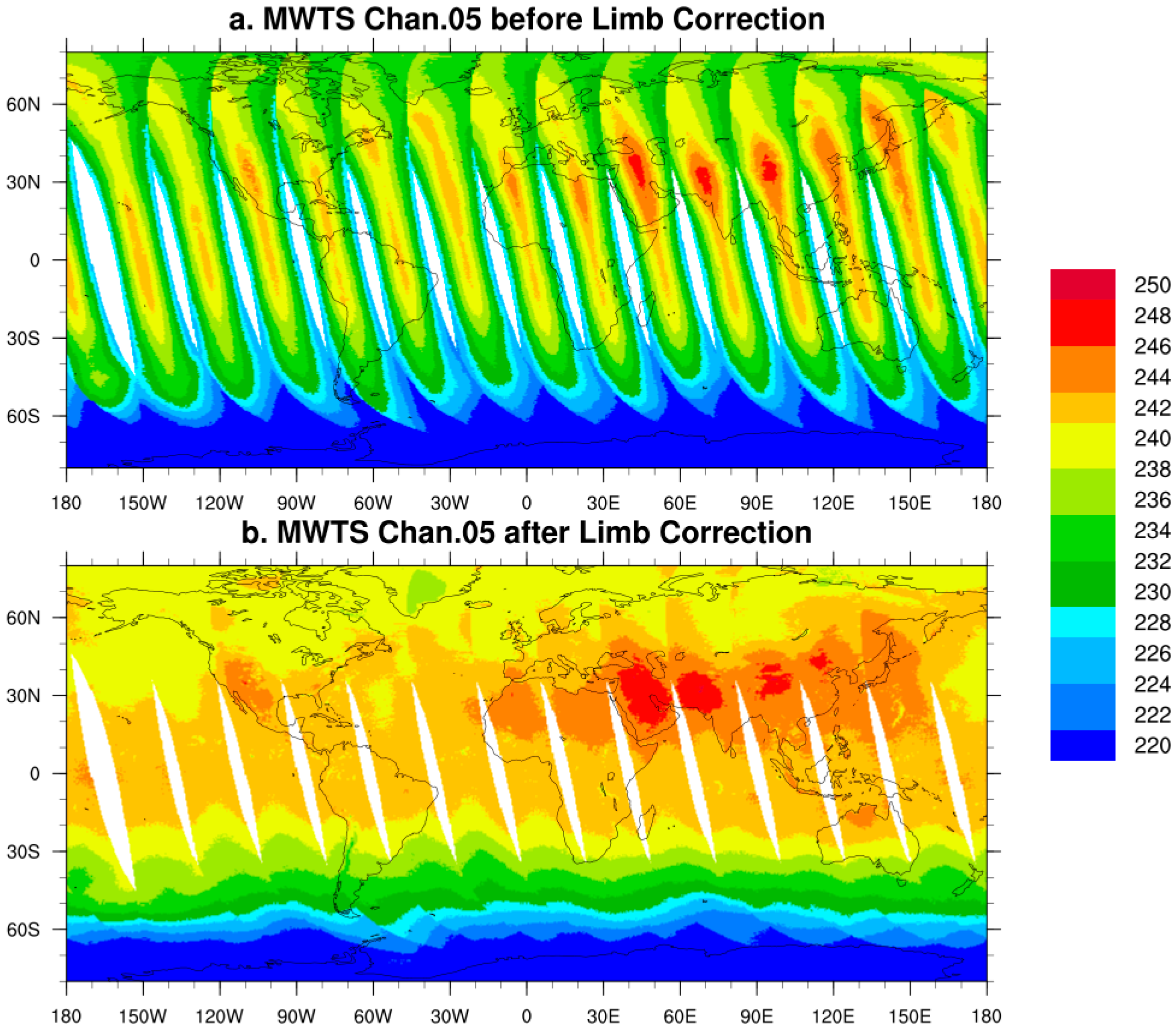
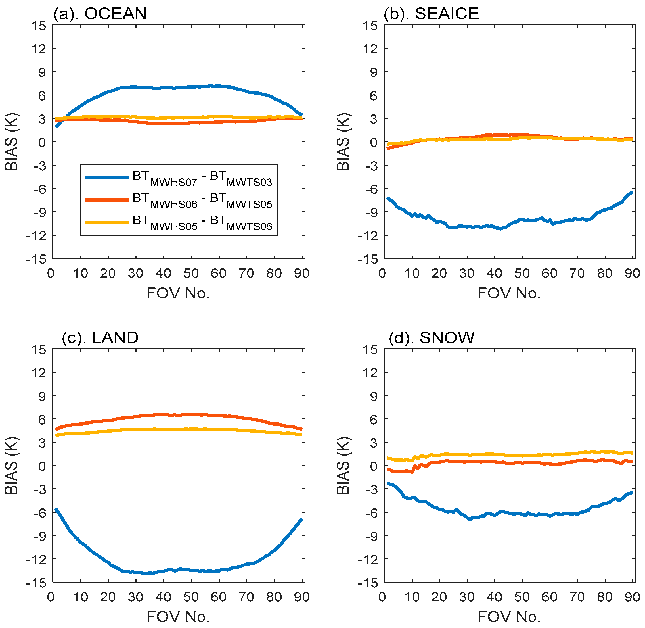
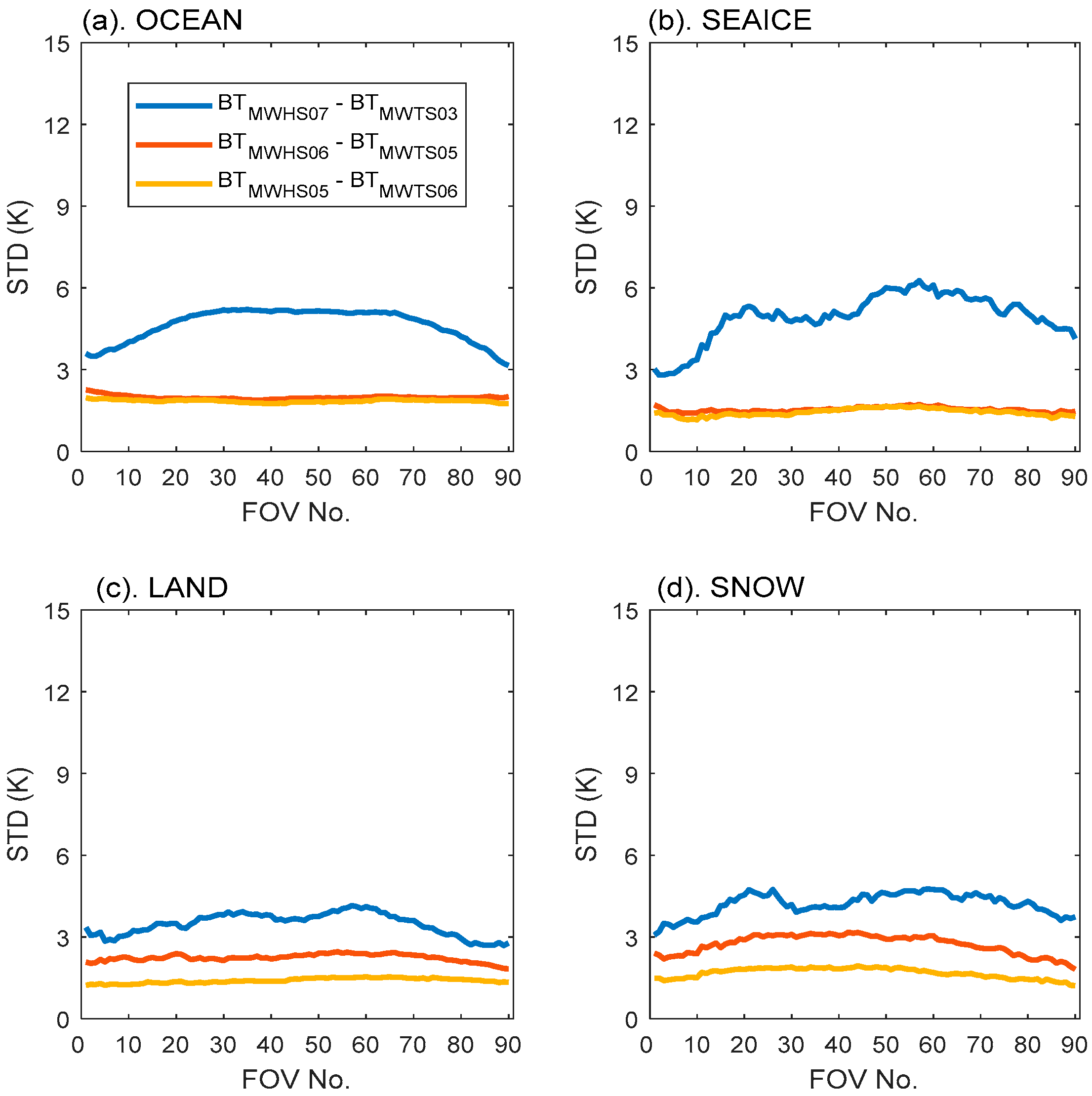
3.2. Limb Correction Algorithm

The microwave sounders of the FY series act as cross-track radiometers, and the observed radiances normally vary with different viewing angles within one scanline. The variation can be up to 15 K at atmospheric temperature channels and even 30 K at the window channels [29]. The feature is called the limb effect, which directly affects the recognition of weather signals. Limb correction is performed as common practice for National Oceanic and Atmospheric Administration (NOAA) operational work, and it is crucial for subsequent applications [30].
The adjustment to limb effect can be derived through physical or statistical methods. The method based on physical and statistical theories was adopted here. The corrections can be performed with the following equation:
y = x T b
where x is the vector of observed brightness temperatures; b is the vector of coefficients trained from an ensemble, and y is the brightness temperatures after the limb correction. The training ensemble consists of the means of x and y over latitude for a long period to obtain a robust result. With the means rather than individual cases of x and y, variations in the brightness temperatures are only caused by the view angle of each beam position. A global set of coefficients were computed and used for least-square fitting for adjustments at a given FOV.
To prevent the limb effect from affecting the cloud identification, the limb corrections should be performed before the CESI calculations. Four-month data for January, April, July and October were selected to compute mean brightness temperatures over each 1° latitude for each FOV. In addition to the channels that were used for correction, another two adjacent channels are selected as well as predictors based on the weighting function [31]. When training the coefficients, the pixel was trained when the sample number over ocean was greater than one hundred. Otherwise, the coefficient of the neighboring latitude at the same FOV was directly used. The global brightness temperatures for MWTS channel 5 before and after limb corrections are displayed in Figure 2. It is clear in Figure 2a that the original global brightness temperatures have obvious scan patterns in each swath. In contrast, the bias and incoherence between neighboring swaths were smoothed after corrections. In consequence for the limb correction, some large-scale weather signals are displayed in the global temperature field.

4. Analysis and Validation
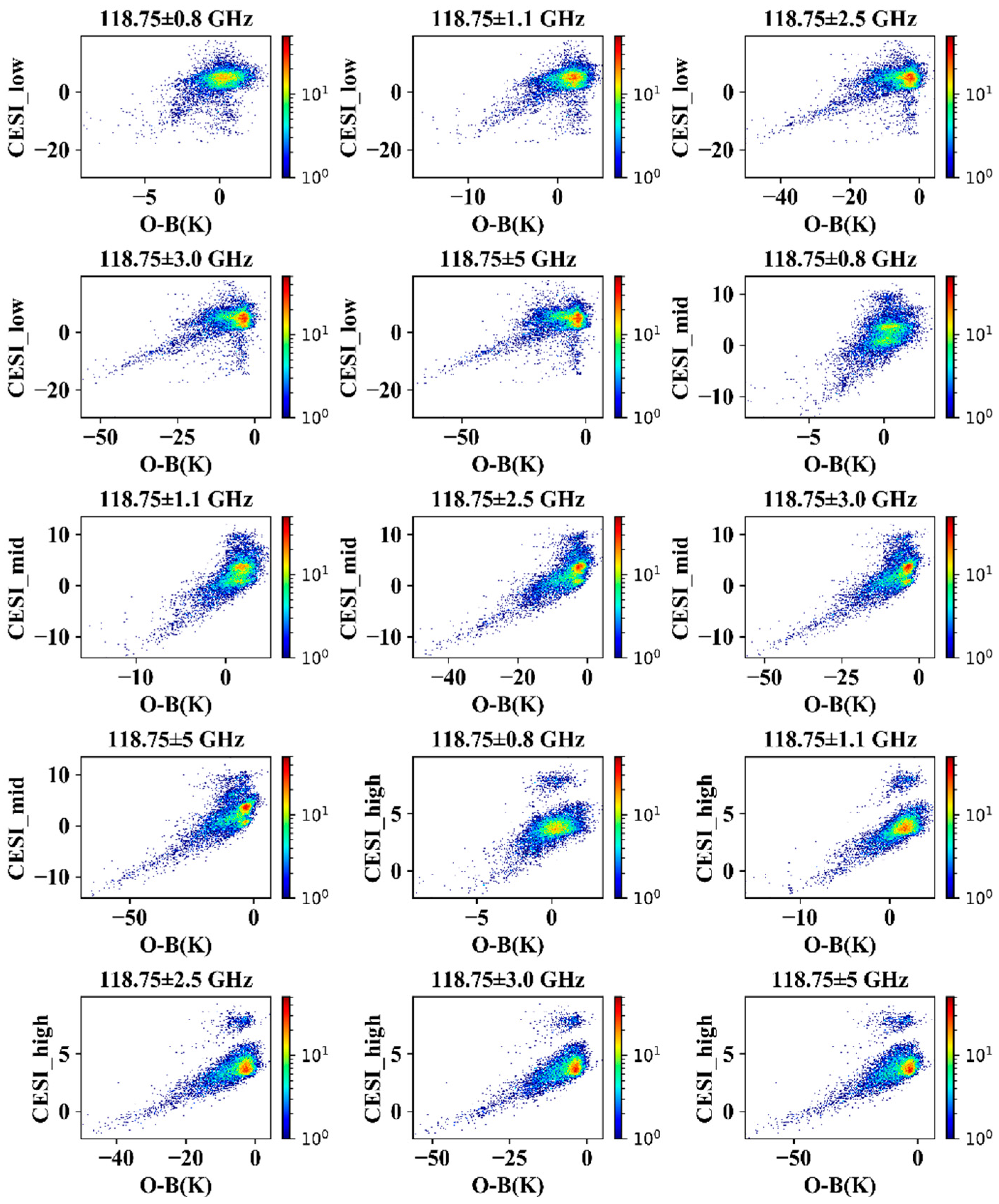
4.1. Analysis

For further discussions of the cloud detection method, accurate temporal and spatial collocations for the MWTS, MWHS, and GPM data are required. The collocation criteria for the temporal and spatial differences were 5 min and 15 km, respectively. Taking the four-month data of January, April, July and October as an example, the total collocated sample number is 1,055,142. According to the surface classification products that were provided by the GPM, four kinds of surfaces were considered. The collocated sample number over the ocean, sea ice, land and snow are 724,173, 78,622, 186,072 and 66,275, respectively.
The ECMWF ERA-5 data for the same period as the MWTS, MWHS and GPM data were used as forward model inputs. Figure 3 provides the scatterplots of the observed brightness temperatures after the limb corrections for three sets of paired channels over four surface types under clear sky conditions. The definition of a clear sky condition is based on the GPM products. It was considered as clear only when the rain rate was equal to zero and the liquid, ice and rain water paths were less than 0.1. It is noticed that only the zenith angle that is less than 10° is in the regions of interest. The correlation coefficients, mean bias and standard deviation are marked in the figure as well. The total number of collocated data is 11,790 (snow), 30,848 (land), 107,469 (ocean) and 13,020 (sea ice).
As shown, the correlation coefficients for most of the pairs are greater than 0.95. The correlation coefficient is 0.91 over sea ice for CESI low . The worse correlation performance is likely due to the limb effect correction coefficient training process. As mentioned above, only the datasets over the ocean surface were trained. Since the high-latitude regions are mostly covered with sea ice, the coefficients were mostly trained using mid- and high-latitude ocean data. In addition, the standard deviation for CESI high is always the lowest among the three pairs, regardless of the surface type.
For further investigations, the bias and standard deviation of three paired channels are given in Figure 4 and Figure 5, respectively. The X-axis is the FOV number. For Figure 4 and Figure 5, the blue, red and yellow curves in subfigures (a)–(d) represent the results for CESI low , CESI mid and CESI high , respectively. It is clear that there is an obvious angular-dependent characteristic for the lower troposphere, while the angular dependence of CESI mid and CESI high is weak. The pattern displays a symmetric bias with respect to the position of the nadir. Moreover, the angular dependence occurs not only in the bias figures (Figure 4), but also in the standard deviation results (Figure 5). The angular-dependent linear regression should be considered. Meanwhile, the insignificant differences in the figures should be eliminated as well.
According to Equations (1) and (2), an angular-dependent correction of the brightness temperature was added, and the final form is shown below as:
CESI i f o v = T B H ( r e g T B H s t d T B i f o v ) = T B H ( α i f o v T B T + β i f o v s t d T B i f o v )
Different from the regression method in Han et al. [11], the coefficients are generated by a simple linear fit between the MWHS and MWTS observations rather than by simulations. The simulations that were calculated from the RT model cannot reflect the possible system bias of the corresponding channels. Therefore, in the actual situation, we believe that it is more effective to use both of the observations to perform the fit. Moreover, to eliminate the variation between the scan positions, the fit was performed in each FOV, and the standard deviation for each scan position was removed as well.

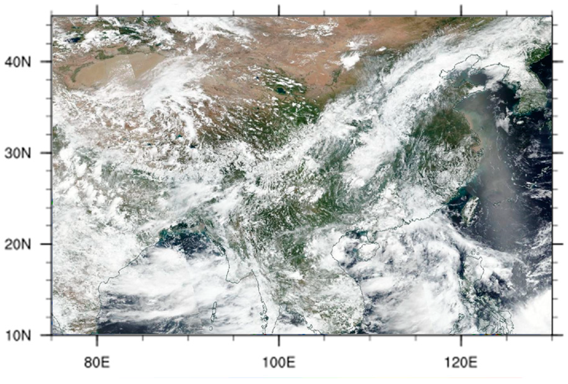
4.2. Validation on the Spatial Distribution

To test the sensitivities to the different surfaces, the landfall process of Typhoon MANGKHUT on 16 September 2018 was chosen. The limb effect on the brightness temperature was adjusted as well. The CESIs that are derived from the dual oxygen absorption bands were initially evaluated through the comparisons with the GPM’s total water products. The time difference between FY-3D and GPM is around 30 min.
Figure 6 compares the spatial distributions between the CESIs and GPM products. The GPM total water product at the corresponding height was selected based on the weighting function peak height of the matched channels. It is shown that the eye, eyewall and rain bands of MANGKHUT are captured well by CESIs. However, there are several false-alarm signals along the coastline which were recognized by CESI low in Figure 6a. Since the matched channels of CESI low are window channels, it was significantly affected by the underlying surface. In contrast, due to the higher weighting function peak, the CESI spatial distributions of CESI mid and CESI high showed more similarities to the GPM total water product.
To further demonstrate the dependence of the CESI algorithm on the surface type, the Tibet Plateau was selected as a special case for discussion. Figure 7 provides the CESI distributions for 17 July 2018. The temporal collocation criterion was about 4 h between GPM and FY-3D observations. Due to the lack of measurements of the GPM data over the plateau or snow cover, the GPM products and cloud images from the Visible Infrared Imaging Radiometer Suite (VIIRS) onboard Suomi NPP (SNPP) satellite are provided as a reference.
In Figure 7a, the algorithm recognized some clouds over most of the land and ocean surfaces. However, it was hard to detect the clouds at high elevations such as the Tibetan Plateau since the weighting function peak of CESI low was already lower than the surface altitude was. What is received is the surface information, rather than the atmospheric scattering information. With an increase in the weighting function peak of CESI mid , this situation was improved. The cloud distribution is closer to the GPM total water distribution in Figure 7d, and it is even much closer to the VIIRS cloud image (Figure 8). It should be noticed that the height that is shown in GPM products is based on the surface altitude. Considering the altitude of the plateau itself, the product height of Figure 7d is much closer to the weighting function peak of CESI mid . CESI mid can well capture the clouds on the plateau. The algorithm fully characterizes the clouds around the mountains. The lack of cloud information in the southeast for the GPM total water products resulted from the relatively large time gap between the GPM and the FY-3D observations.
Figure 6. Spatial distributions of CESIs derived from (a) CESI low , (b) CESI mid and (c) CESI high on 16 September 2018. The spatial distributions of GPM total water product are shown at (d) 0.5 km, (e) 6 km and (f) 9 km.
Remotesensing 14 05332 g006
Figure 7. Spatial distributions of CESIs derived from (a) CESI low , (b) CESI mid and (c) CESI high on 17 July 2018. The spatial distributions of GPM total water product are shown at (d) 0.5 km, (e) 6 km and (f) 9 km.
Remotesensing 14 05332 g007
Figure 8. Cloud images from the VIIRS onboard SNPP.
Remotesensing 14 05332 g008

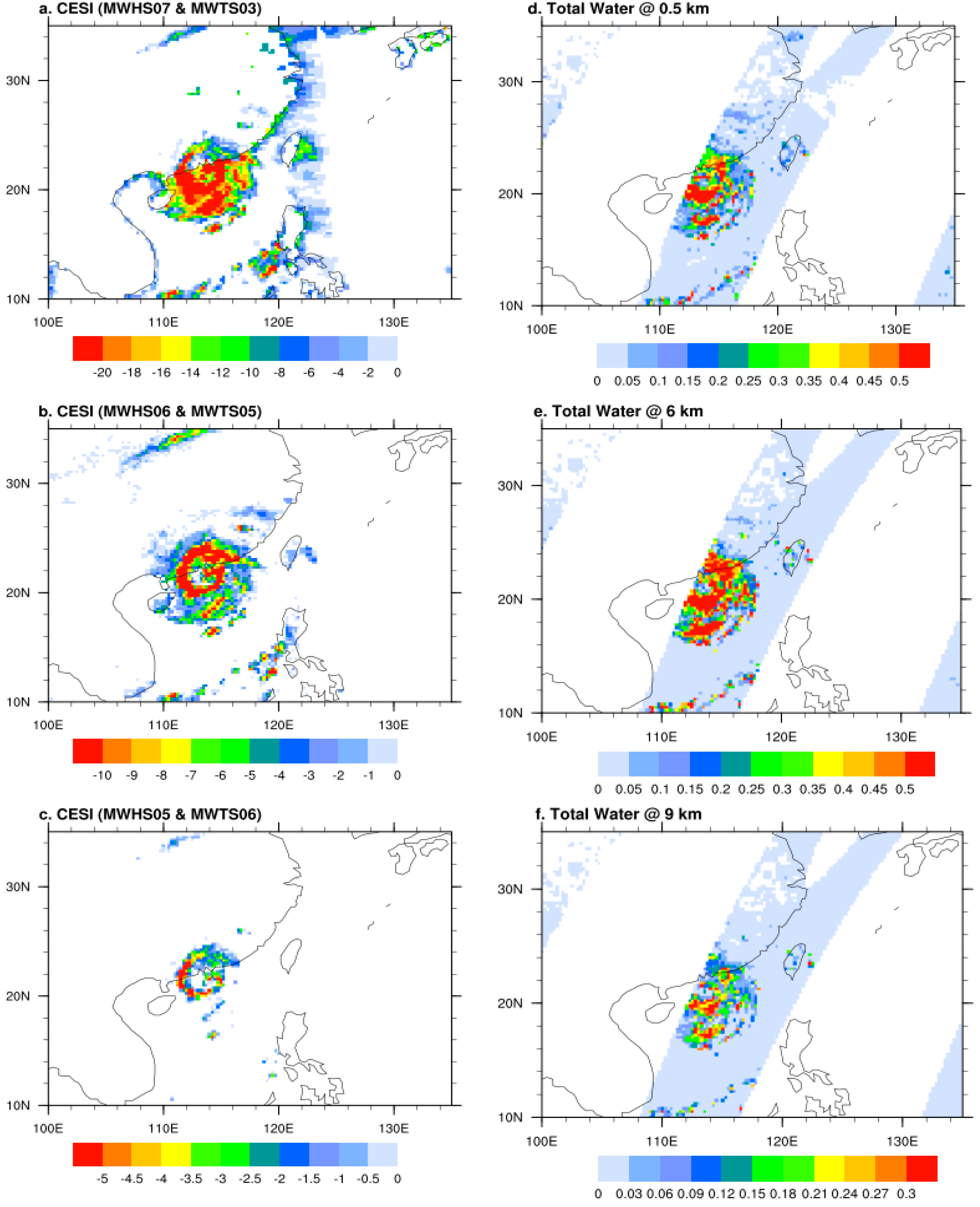
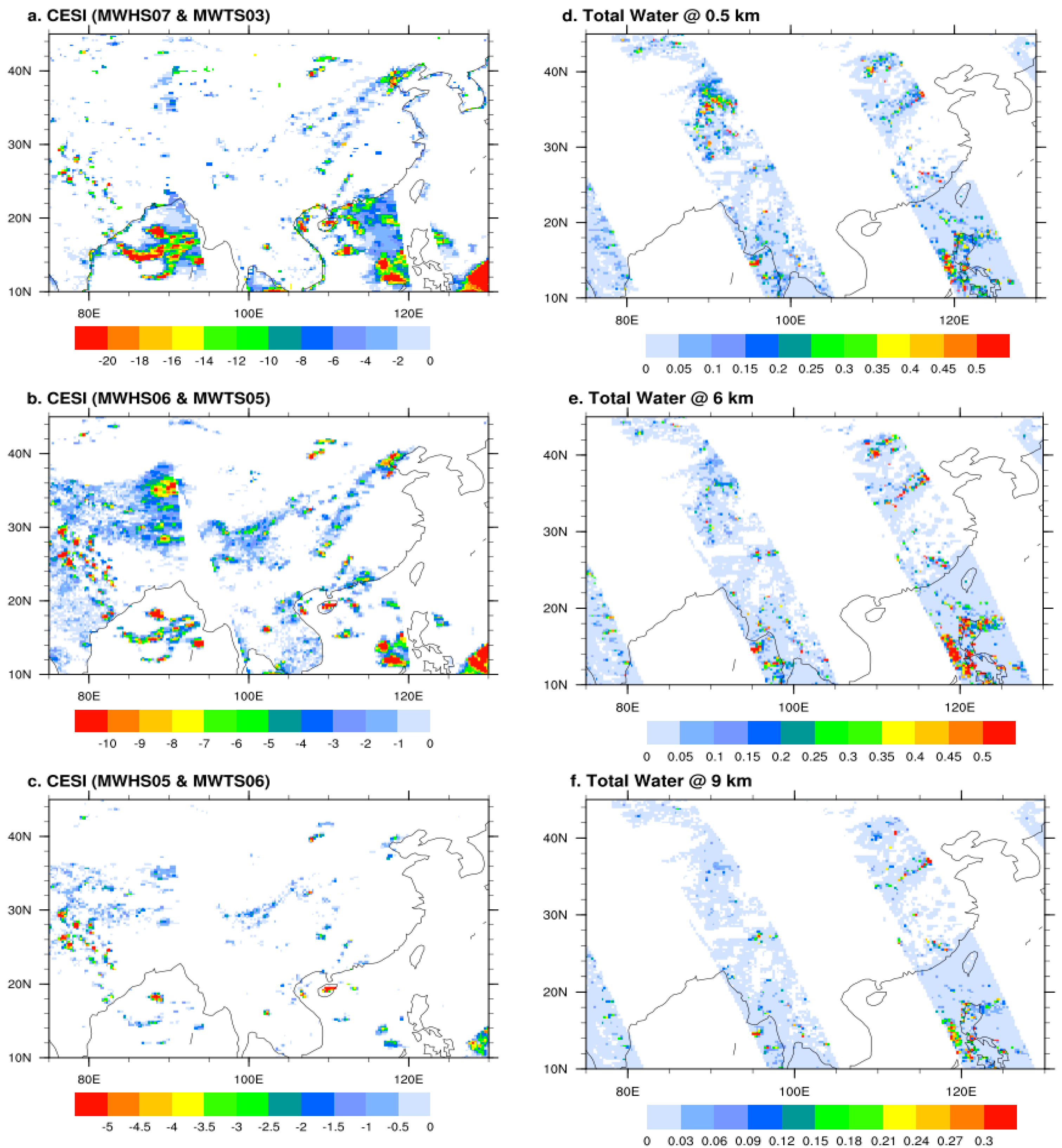
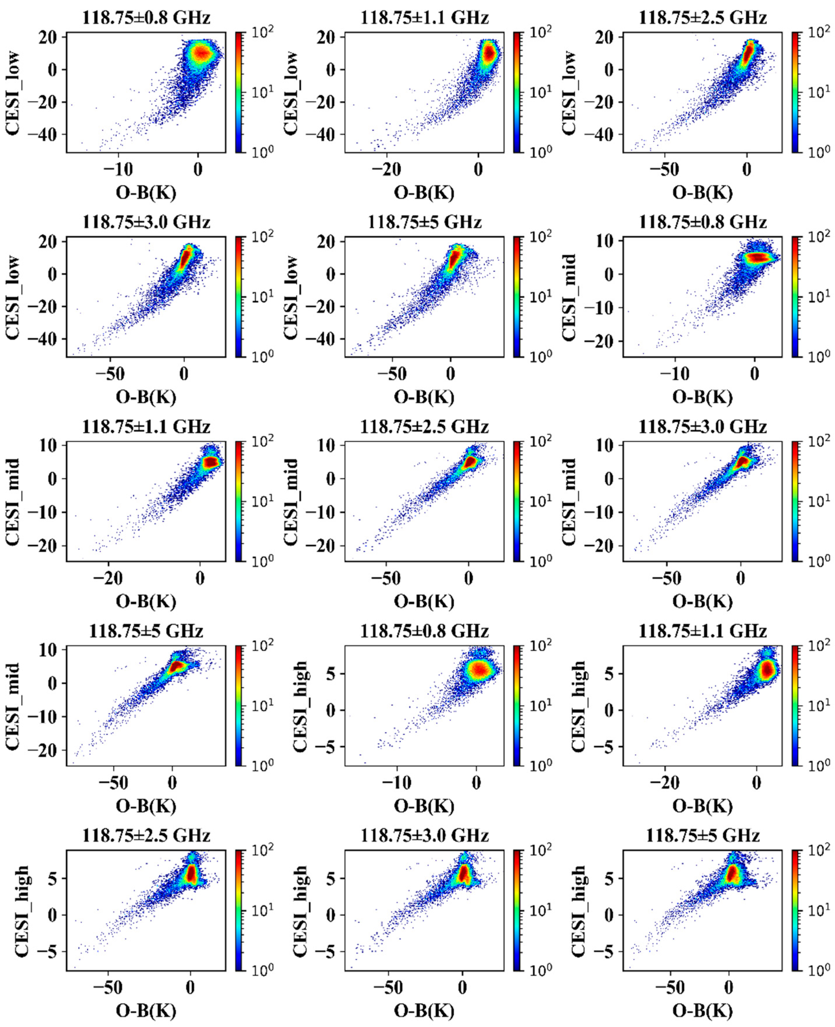
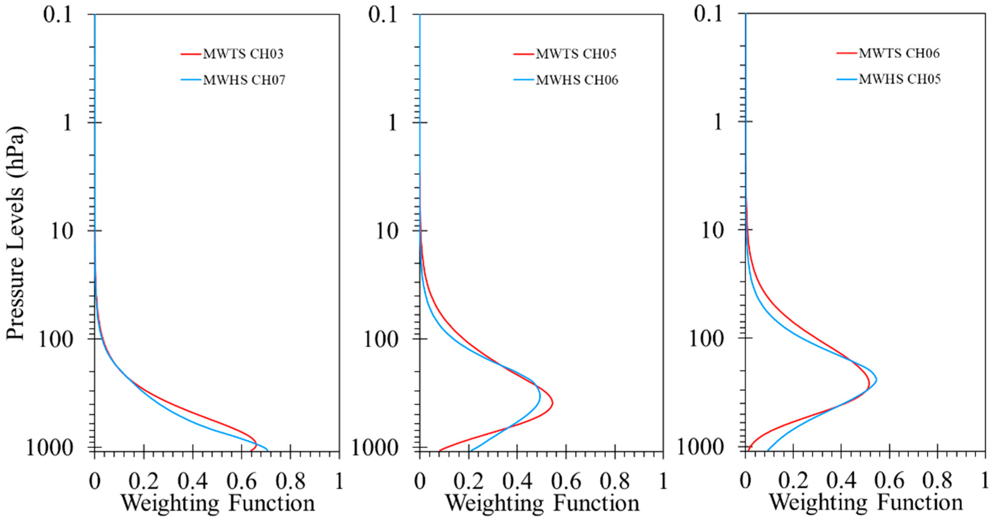
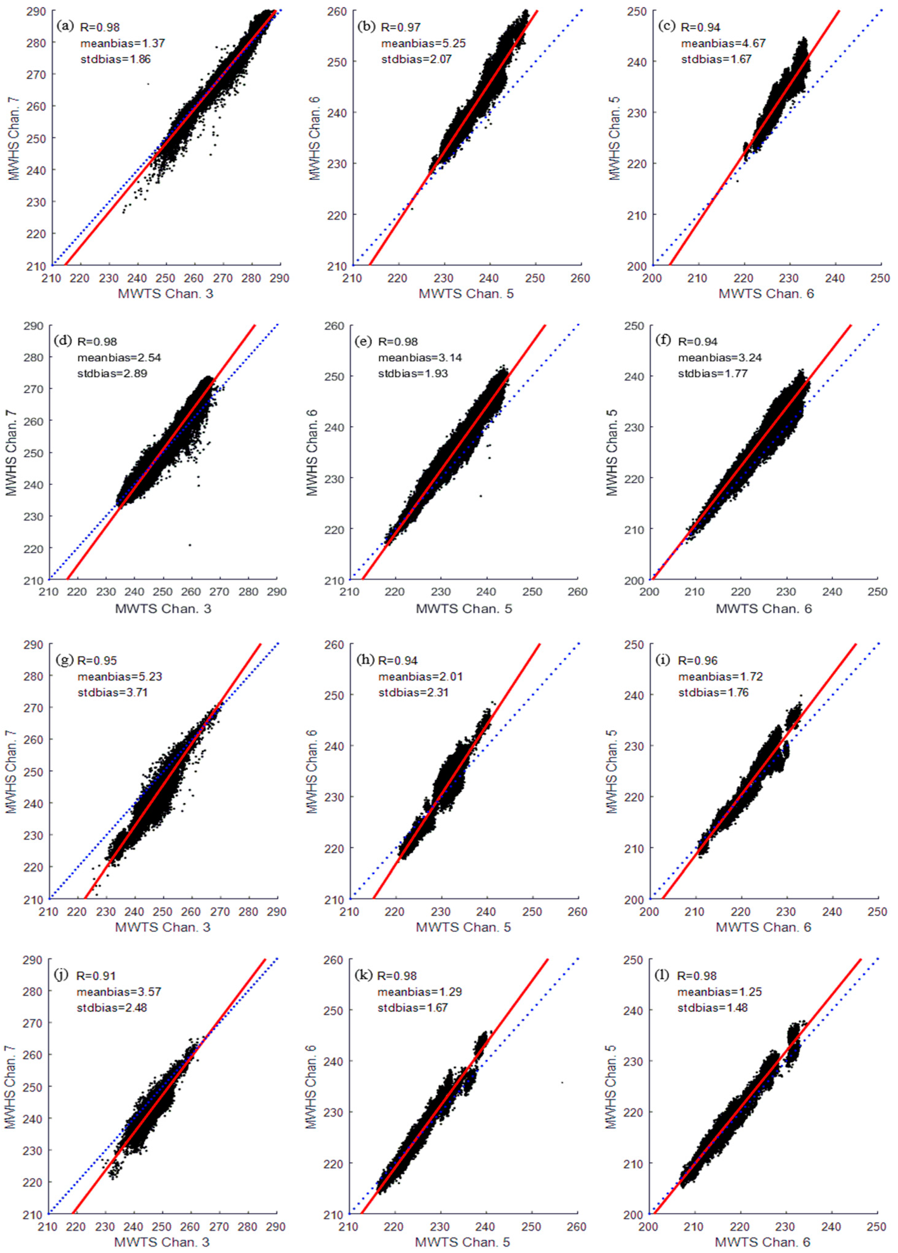
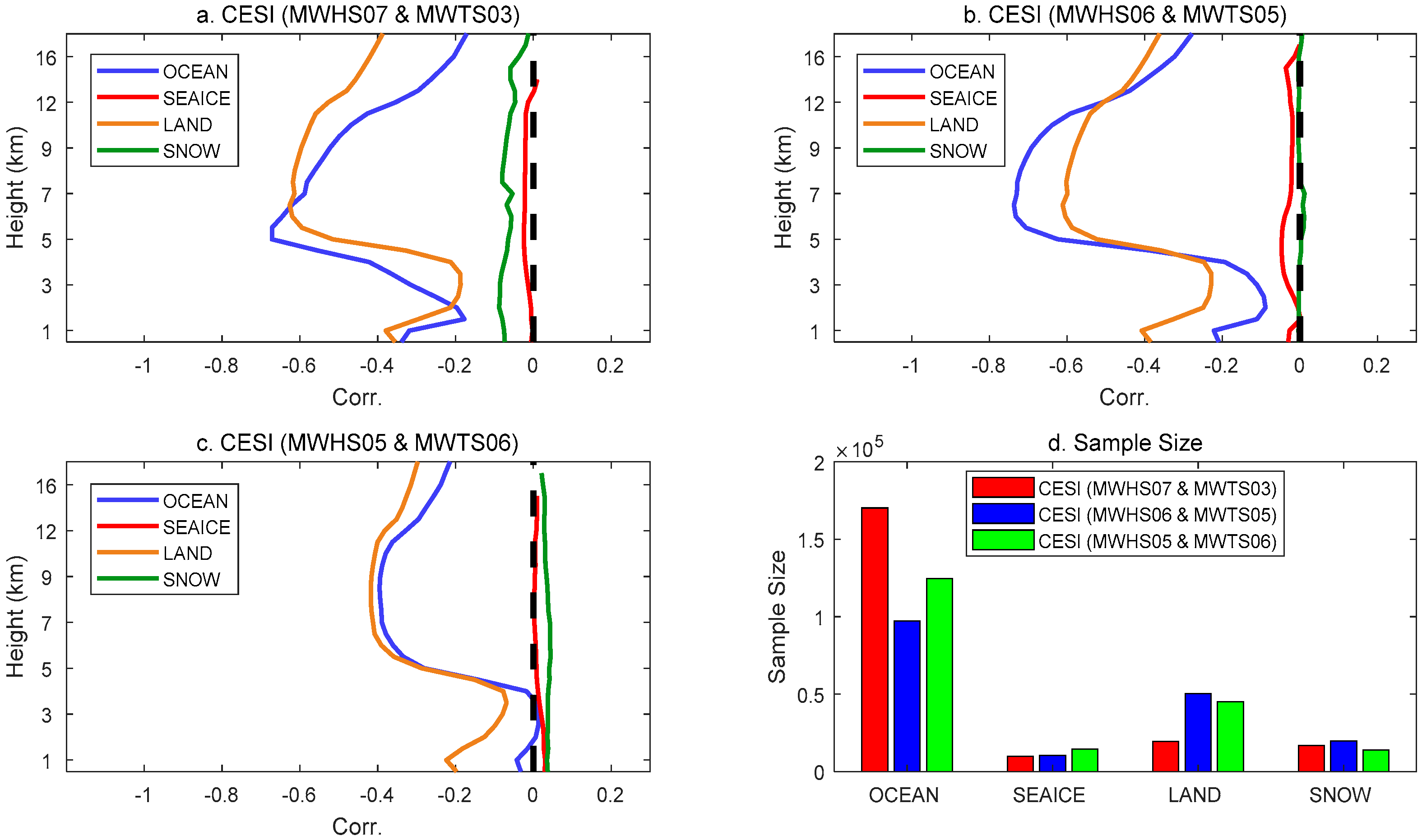
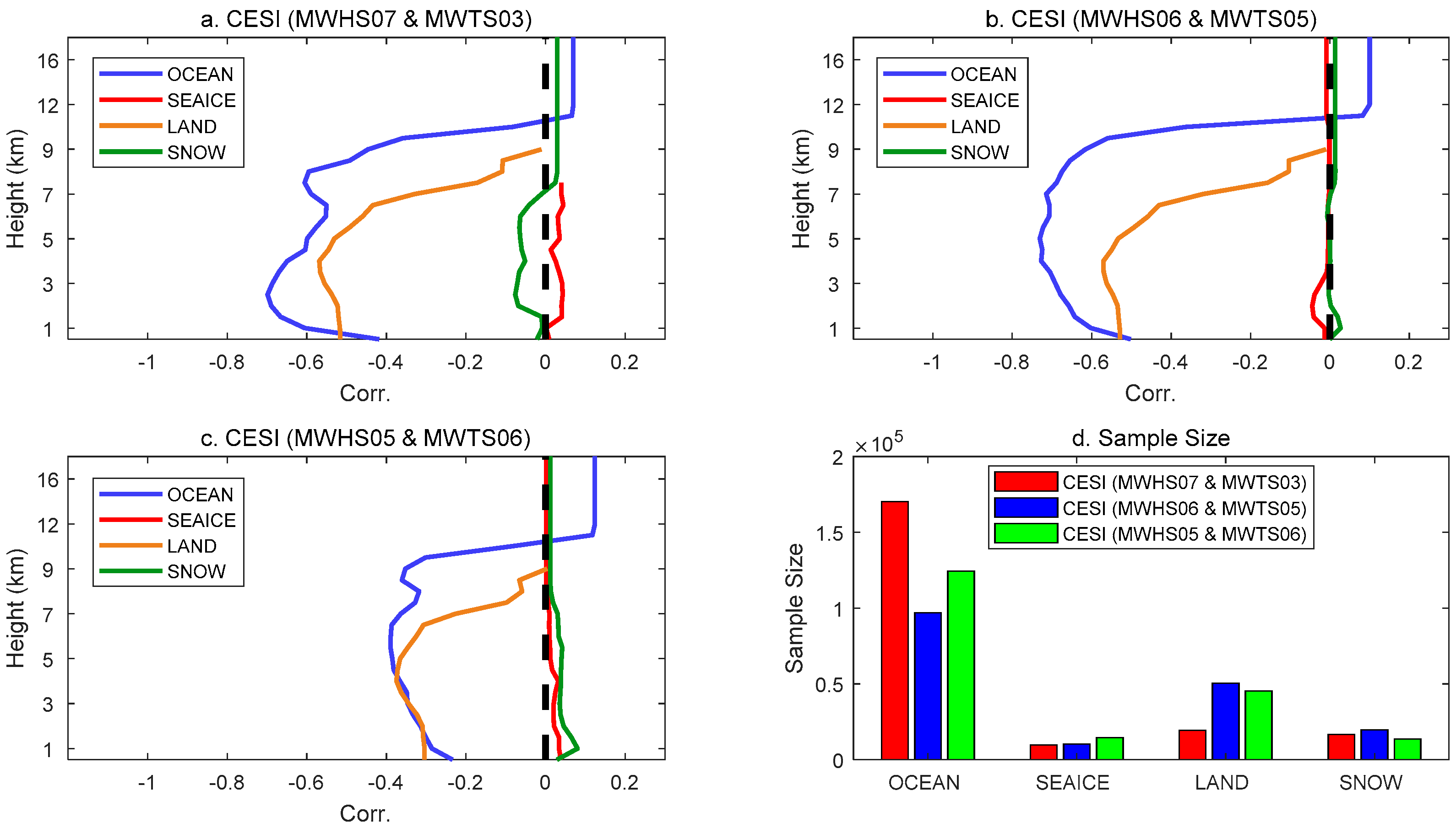
4.3. Validation of Verical Distribution

The CESI algorithm can depict not only the spatial distribution, but also the vertical distribution of the clouds. In order to quantitatively evaluate the accuracy of the CESI vertical distribution, the GPROF hydrometeor profiles can be used as the standards for the examinations. The testing collocation dataset is independent of the regression coefficients for the independent validation. In this way, a relative reliable validation was completed.
The GPROF hydrometeor profiles were used as references to examine the vertical distributions of CESIs over different surface types. The product has four kinds of water type: liquid water, ice, rain and snow. Due to the inaccuracy of ice retrieval, only the snow type was considered as a solid profile. The correlations of three different profile types were estimated.
Validated by the four-month collocation data (February, May, August and November), the sample size comprises over 10 thousand data points over the different surface types of each CESI pair. Figure 9, Figure 10 and Figure 11 show the correlations of the solid, liquid and total profiles, respectively. The solid profile was used for comparisons first. The blue, red, brown and green curves in the figure represent the results under the ocean, sea ice, land and snow conditions, respectively. The dashed black line represents the zero value. As shown in Figure 9, the correlation coefficients over the land and ocean are greater than that over the snow and sea ice. The vertical distribution of the solid profile over the land is similar to that over the ocean. It is clear that the correlation coefficient is up to about 0.7 at about 5 km height, and this decreases from that height to the surface. The sharp decrease of the correlation coefficients below 5 km may be due to the melting of the solid particles. Among the three pairs, CESI mid had a better recognition effect on the height range of 5–12 km, and the algorithm was more accurate over ocean among the height range. For the liquid profile consisting of liquid water and rain, the general situation is the same as a solid profile in Figure 10. Since there is no liquid presence above a certain altitude, the correlation coefficients are close to zero above 10 km. The maximum correlation coefficient is about 0.8, which is consistent with matched channels’ weighting function peak. The correlations of the total of three hydrometeor profiles were estimated as well. The shape of CESIs over the ocean in Figure 10 is more consistent with the channel weighting functions. Considering the complexity of the terrain over land, the lower correlation coefficients are understandable. However, CESI low and CESI mid correlate well between 5–12 km. In addition, the CESIs over the snow and sea ice have a low correlation under all of the conditions, and their values are remarkably similar. Thus, it is hard to identify the clouds over the snow and sea ice surfaces.
Generally, the CESIs almost have a negative correlation with the GPROF profiles over all of the surface types for all of the pairs. The algorithm has a higher accuracy with the GPROF profiles at a paired channel weighting function peak height over the ocean. The variations between the CESI pairs over the land surfaces are not obvious. Overall, CESI high of the MWHS channel 5 and MWTS channel 3, representing the higher troposphere scattering information, correlates worse than the other pairs do.

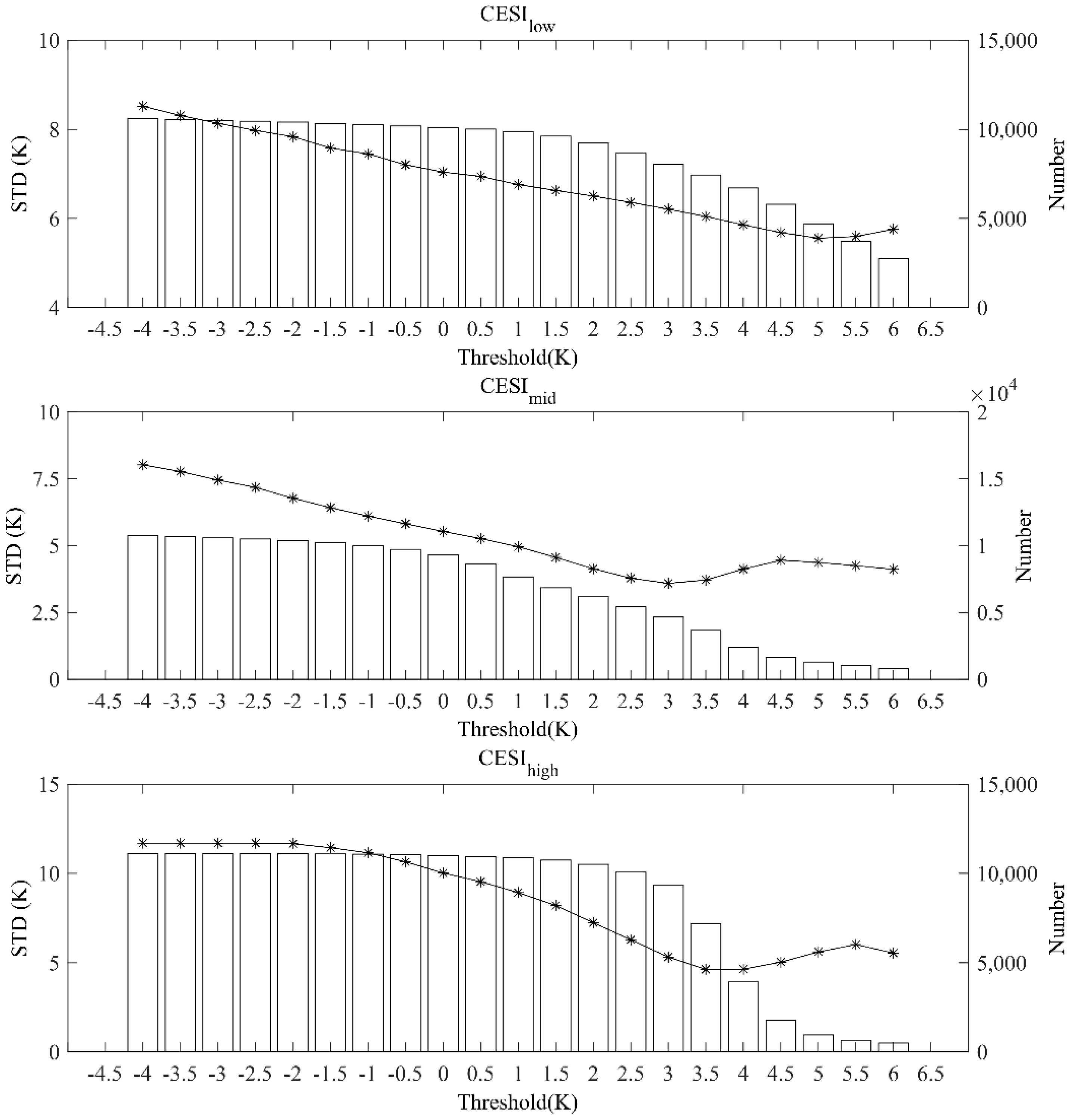
4.4. Discussion on Cloud Detection Thresholds

In previous analysis and validations, the CESI scheme has a relatively good detection performance over the ocean and the land. However, the thresholds for the cloud scattering indices were not discussed specifically, and a zero threshold was used to determine the cloud for all of the layer heights. To further determine the threshold selection for the CESIs at different heights and surface types, channels 5–9 around 118 GHz of the MWHS, which are sensitive to the tropospheric information, were selected for the analysis. The microwave sounder data from 20 July 2021 and the atmospheric profile from the ERA5 reanalysis data were used as the inputs for the brightness temperature simulation under the clear sky conditions. A preliminary threshold range determination was performed by considering the relationship between the CESIs and the observations minus the simulations (O − B) at different height layers over the ocean and land. The collocated sample numbers over the ocean and the land are 31,109 and 15,103, respectively.
The correspondence between the CESI low , CESI mid , CESI high and O − B values over the ocean are illustrated in Figure 12. The CESIs for each channel show a good linear relationship with the O − B values regardless of the layer height. The plots for the middle and upper layers show a more pronounced relationship between the CESIs and the O − B values than they do for the lower layers due to the higher weighting function peak. Overall, for these five different oxygen absorption channels, the points of each channel O − B near zero are concentrated in almost the same position, corresponding to a certain range of CESI. This feature is shown on the plots of different layers, which was the basis for the subsequent preliminary classification of clear sky and cloudy areas.
Figure 13 shows the correspondence over the land surface. A linear relationship between the CESIs and O − B values is less pronounced for each channel over land than it is over the ocean. In particular, for the lower layers, the CESI may be more influenced by the surface emissivity, with a wide range from negative to positive, corresponding to the value of zero for O − B. This irregularity is improved by the correspondence of the CESI mid , which corresponds best to the O − B. In general, for these five chosen channels, the correspondence between the CESIs and O − B values for each layer over the land surface still shows a clear linear relationship, and the concentration of points with O − B values around zero observed in Figure 12 are still reflected.
According to the relationship between the CESIs and the O − B values in Figure 12 and Figure 13, the range of the CESI when the O − B value is close to zero was roughly determined. A range from -4 K to 6 K was performed at 0.5 K intervals to test the threshold values of the CESIs at different layers. Taking the window channel of the MWHS (channel 10, 150 GHz) as an example, Figure 14 shows the situations for the screened-out clear sky points by the corresponding thresholds. The curves in the figure indicate the change in the standard deviation of the clear sky points after the screening, while the bars indicate the remaining number. For the near-surface-sensitive CESI low channels, the standard deviation follows a monotonic trend with respect to the threshold. The larger the threshold is, the smaller the standard deviation of clear sky points is, but the number of points decreases slowly, whereas the CESI mid and CESI high behave differently from the CESI low . As the threshold increases, the standard deviation value first decreases abruptly. However, the standard deviation remains almost constant or even increases after reaching a certain value. The number of remaining points after the screening also varies significantly. In order to achieve a balance between the number and the standard deviation, the thresholds for the different height layers of the ocean surface were taken as 6, 3.5 and 4.5, respectively.
Figure 12. Scatter density plots of cloud scattering index versus five channel observation versus O − B values on the ocean surface for different height layers, where the color scale indicates the density of points.
Remotesensing 14 05332 g012
Figure 13. Same as Figure 12 except for the land surface.
Remotesensing 14 05332 g013
Figure 14. The standard deviation of O − B values (lines with asterisks) and the remaining number (bars) of MWHS channel 10 (150 GHz) in the clear sky region over ocean surface. The clear-sky points are screened out by the corresponding threshold.
Remotesensing 14 05332 g014
The threshold determinations for the land surfaces are generally similar to those for ocean surfaces (Figure 15). However, there are differences in the threshold identification for the surface-sensitive CESI low channels. As the threshold changes from −4 K to 2 K, the remaining number of points changes relatively little as the standard deviation decreases. As the threshold increases to 5 K, the number of points decreases more. The standard deviation tends to increase as the threshold value increases further. For the CESI mid and CESI high , the number of points decreases dramatically after the threshold values were taken as 0 and 2.5, respectively. The standard deviations all show a decreasing trend, then an increasing one and then, a decreasing one again with the increasing threshold values. Although it is within the range of values, the standard deviation of the clear-sky points has a minimum value at the different layers. The final thresholds for the land surface identification were set as 1, 3 and 3 in consideration of the remaining number of clear-sky points.
The probability density distributions of clear sky points that were filtered by the newly established thresholds were compared with those with the clouds to verify the effectiveness of the newly established thresholds. The blue part of the figure indicates the probability density distribution of the filtered clear sky points, and the pink part indicates the probability density distribution of the rejected cloudy points. Since the window channels were more severely affected, while the channels with the weighting function peak in the stratosphere were hardly affected by the clouds, only few channels are shown. The frequency settings of each channel are labelled at the top of the figure.
In Figure 16, it can be seen that the probability distribution of the screened clear sky points basically satisfies the characteristics of a normal distribution, and the O − B value corresponding to the highest probability density of the screened clear sky points in each channel is almost around zero. Among the five oxygen absorption channels around 118.75 GHz, the remaining channels can effectively distinguish the clear sky from the cloudy information, except for the 118.75 ± 0.8 GHz and 118.75 ± 1.1 GHz channels with the weighting function peak being higher. Although there is some overlap between the probability density graphs of the clear sky and the cloudy information for this channel, the overall O − B distribution for the clear sky points is concentrated within a smaller region that is around zero. The overlap may be due to the inaccurate selection of the clear sky points that is caused by the channel’s insensitivity to the cloud information below the weight height. The same principle can also explain the phenomena of the channels at 54.4 GHz, 54.94 GHz and 55.5 GHz. For these channels, it can be approximated that the observation as taken under a clear sky. Among the 15 channels shown, the CESI scheme is ineffective in distinguishing clear sky from cloudy information at 52.8 GHz and 183.31 ± 1 GHz. However, in general, the O − B values of the screened clear sky points remain low. For most channels, the probability density distribution of the screened clear sky data approximates a Gaussian distribution.
Similarly, Figure 17 shows the probability density distribution of the O − B values of the screened-out clear sky points over the land versus the rejected cloudy points. In general, the distinction between the clear sky and the cloudy information is not very clear over the land surface. The graphs of the probability density distributions of O − B for clear sky and cloudy for most channels overlap. Similar to the case over the ocean, the four channels from 53.596 GHz to 55.5 GHz can be approximated as a clear sky due to the overall small O − B values. Similarly, the channels at 52.8 GHz and 183.31 ± 1 GHz are not very significant in distinguishing the clear sky from the presence of clouds. Over a land surface, the large O − B values of the screened-out clear sky points at 52.8 GHz may be due to the ground sensitivity of the channel. The CESI identification scheme is heavily influenced by the complex terrain as well as the land emissivity. Overall, although the recognition of land is not as good as it is for an ocean surface, it can basically meet the recognition requirements.

5. Conclusions

A combination use of the dual oxygen absorption bands offers a unique chance for cloud screening to be performed. Three pairs were matched based on the weighting functions of each channel, and these represent the scattering information of the upper, middle, and low troposphere, respectively.
Due to the scanning characteristics of the microwave sounders, limb effect corrections should be performed before the CESI calculations are performed. As a result, the limb effect can be mostly removed, and weather signals are revealed more clearly after the corrections. With the four-month data for the CESI coefficients training, a detailed analysis of the algorithm sensitivity to the underlying surface was conducted. Three paired channels correlate well across most surface types with the ARMS simulations under a clear sky. The poor effect over the sea ice surface was caused by the training process of the limb effect correction coefficients. An additional angular dependence was eliminated as well. It is revealed that the spatial distributions of the CESIs show a high degree of similarity with the GPM products both over the oceans and the land, except around the coastline in the case of typhoon MANGKHUT. Taking the Tibetan Plateau as a special terrain example, the cloud information is well captured by CESI mid and is close to the VIIRS cloud image.
For a quantitative assessment of the CESI vertical distribution, independent validations were conducted using GPROF hydrometeor profiles as references. The correlation relationships over the sea surface were consistent with weighting functions of the paired channels. In contrast, there are slight variations in heights between the results of the CESI pairs due to the complexity of the land surface. It should be noted that this method is difficult to distinguish the clouds over sea ice and snow.
Different surface types are specifically discussed to choose further the thresholds of the CESI scheme at different heights. Based on the relationship between the CESIs and O − B values, the threshold selection range was determined, and the test threshold was performed at 0.5 K intervals. The combination of the thresholds for different heights was selected to be used for the scheme to achieve the best possible balance between the number and standard deviation of the remaining clear-sky points. According to the analysis, the thresholds for the different height levels were 6, 3.5 and 4.5 over the ocean and 1, 3 and 3 over the land. In the validation of the effect of the new threshold, the probability density distribution of the selected clear-sky data approximates a Gaussian distribution in most of the channels. The high weighting function peak height may cause poor recognition results for some channels. The setting of the thresholds in the subsequent study can be carried out further by considering the characteristics of the different channels.
Overall, the improved CESI algorithm is suitable for all of the surface types, including plateaus. It can accurately capture the spatial and vertical distribution of clouds. The results also show that the new threshold combination can be effective for cloud identification. Moreover, the CESI scheme can better use the different detection capabilities of the two microwave instruments, and it provides a new idea for quality control in data assimilation. It is valuable not only for the microwave sounding instruments onboard FY-3D but also for those on onboard FY-3E. With similar channel settings, this method can be easily implemented to the FY-3E microwave sounding instruments with a training of new coefficients of the CESI.

Author Contributions

Conceptualization, H.H. and F.W.; methodology, H.H. and F.W.; validation, W.K. and H.H.; resources, W.K. and H.H.; writing—original draft preparation, W.K.; writing—review and editing, H.H. and F.W. All authors have read and agreed to the published version of the manuscript.

Funding

This research was funded by the National Key Research and Development Program of China (2021YFB3900400), the National Nature Science Foundation of China (Grant No. 42105136, No. 41905036 and U2142212).

Data Availability Statement

The FY3D satellite data can be downloaded from the website of China National Satellite Meteorological Center (http://satellite.nsmc.org.cn/portalsite/default.aspx (accessed on 23 October 2022). The level 2A GMI GPROF dataset can be downloaded from the website of NASA STORM (https://storm.pps.eosdis.nasa.gov/storm/ (accessed on 23 October 2022).

Acknowledgments

We thank Jun Yang, Yang Han, and Yining Shi for supporting the usage of the ARMS radiative transfer model. We would also like to thank the reviewers and the editors for their valuable and helpful suggestions.

Conflicts of Interest

The authors declare no conflict of interest.

References

  1. Migliorini, S.; Candy, B. All-sky satellite data assimilation of microwave temperature sounding channels at the Met Office. Q. J. R. Meteorol. Soc. 2019, 145, 867–883. [Google Scholar] [CrossRef]
  2. Kan, W.; Han, Y.; Weng, F.; Guan, L.; Gu, S. Multisource Assessments of the FengYun-3D Microwave Humidity Sounder (MWHS) On-Orbit Performance. IEEE Trans. Geosci. Remote Sens. 2020, 58, 7258–7268. [Google Scholar] [CrossRef]
  3. Carminati, F.; Atkinson, N.; Candy, B.; Lu, Q.F. Insights into the microwave instruments onboard the Feng-Yun 3D satellite: Data quality and assimilation in the Met Office NWP system. Adv. Atmos. Sci. 2020, 38, 1379–1396. [Google Scholar] [CrossRef]
  4. Li, J.; Zou, X. A quality control procedure for FY-3A MWTS measurements with emphasis on cloud detection using VIRR cloud fraction. J. Atmos. Ocean. Technol. 2013, 30, 1704–1715. [Google Scholar] [CrossRef] [Green Version]
  5. Han, H.; Li, J.; Goldberg, M.; Wang, P.; Li, J.; Li, Z.; Sohn, B.-J.; Li, J. Microwave Sounder Cloud Detection Using a Collocated High-Resolution Imager and Its Impact on Radiance Assimilation in Tropical Cyclone Forecasts. Mon. Weather Rev. 2015, 144, 3937–3959. [Google Scholar] [CrossRef]
  6. Qin, Z.; Zou, X. Uncertainty in Fengyun-3C microwave humidity sounder measurements at 118 GHz with respect to simulations from GPS RO data. IEEE Trans. Geosci. Remote Sens. 2016, 54, 6907–6918. [Google Scholar] [CrossRef]
  7. Grody, N.; Zhao, J.; Ferraro, R.; Weng, F.; Boers, R. Determination of precipitable water and cloud liquid water over oceans from the NOAA 15 advanced microwave sounding unit. J. Geophys. Res. 2001, 106, 2943–2953. [Google Scholar] [CrossRef]
  8. Weng, F.; Zhao, L.; Ferraro, R.; Poe, G.; Li, X.; Grody, N. Advanced microwave sounding unit cloud and precipitation algorithms. Radio Sci. 2003, 38, 8068. [Google Scholar] [CrossRef]
  9. Ji, D.; Shi, J.; Xiong, C.; Wang, T.; Zhang, Y. A total precipitable water retrieval method over land using the combination of passive microwave and optical remote sensing. Remote Sens. Environ. 2017, 191, 313–327. [Google Scholar] [CrossRef]
  10. Bennartz, R.; Thoss, A.; Dybbroe, A.; Michelson, B. Precipitation analysis using the Advanced Microwave Sounding Unit in support of nowcasting applications. Meteorol. Appl. 2002, 9, 177–189. [Google Scholar] [CrossRef]
  11. Lin, L.; Zou, X.; Weng, F. Combining CrIS double CO2 bands for detecting clouds located in different layers of the atmosphere. J. Geophys. Res. Atmos. 2017, 122, 1811–1827. [Google Scholar] [CrossRef]
  12. Wang, L.; Tian, M.; Zheng, Y. Assessment and improvement of the Cloud Emission and Scattering Index (CESI)–an algorithm for cirrus detection. Int. J. Remote Sens. 2019, 40, 5366–5387. [Google Scholar] [CrossRef]
  13. Han, Y.; Zou, X.; Weng, F. Cloud and precipitation features of Super Typhoon Neoguri revealed from dual oxygen absorption band sounding instruments on board FengYun-3C satellite. Geophys. Res. Lett. 2015, 42, 916–924. [Google Scholar] [CrossRef]
  14. Hu, H.; Weng, F. Influences of 1DVAR Background Covariances and Observation Operators on Retrieving Tropical Cyclone Thermal Structures. Remote Sens. 2022, 14, 1078. [Google Scholar] [CrossRef]
  15. Lawrence, H.; Carminati, F.; Bell, W.; Bormann, N.; Newman, S.; Atkinson, N.; Geer, A.J.; Migliorini, S.; Lu, Q.; Chen, K. An Evaluation of FY-3C MWRI and Assessment of the Long-Term Quality of FY-3C MWHS-2 at ECMWF and the Met Office; European Centre for Medium-Range Weather Forecasts: Reading, UK, 2017; Available online: https://www.ecmwf.int/sites/default/files/elibrary/2017/17206-evaluation-fy-3c-mwri-and-assessment-long-term-qualityfy-3c-mwhs-2-ecmwf-and-met-office.pdf (accessed on 23 October 2022).
  16. Matsui, T.; Iguchi, T.; Li, X.; Han, M.; Tao, W.-K.; Petersen, W.; L’Ecuyer, T.; Meneghini, R.; Olson, W.; Kummerow, C.D.; et al. GPM Satellite Simulator over Ground Validation Sites. Bull. Am. Meteorol. Soc. 2013, 94, 1653–1660. [Google Scholar] [CrossRef]
  17. Iguchi, T.; Seto, S.; Meneghini, R.; Yoshida, N.; Awaka, J.; Kubota, T. GPM/DPR Level-2 Algorithm Theoretical Basis Document. Available online: http://pmm.nasa.gov/sites/default/files/document_files/ATBD_GPM_DPR_n3_dec15.pdf (accessed on 23 October 2022).
  18. Jackson, G. NASA’s Global Precipitation Measurement (GPM) Mission for Science and Society. In Proceedings of the Egu General Assembly Conference, Vienna, Austria, 17–22 April 2016. [Google Scholar]
  19. Jackson, T.; Walter, A.P.; Gottfried, K.; David, C.G.; David, B.W. Evaluation of global precipitation measurement rainfall estimates against three dense gauge networks. J. Hydrometeorol. 2018, 19, 517–532. [Google Scholar]
  20. Hou, A.Y.; Kakar, R.K.; Neeck, S.; Azarbarzin, A.A.; Kummerow, C.D.; Kojima, M.; Oki, R.; Nakamura, K.; Iguchi, T. The Global Precipitation Measurement Mission. Bull. Am. Meteorol. Soc. 2014, 95, 701–722. [Google Scholar] [CrossRef]
  21. Li, X.; Tao, W.-K.; Matsui, T.; Liu, C.; Masunaga, H. Improving a spectral bin microphysical scheme using long-term TRMM satellite observations. Q. J. R. Meteorol. Soc. 2010, 136, 382–399. [Google Scholar] [CrossRef] [Green Version]
  22. Saunders, R.; Matricardi, M.; Brunel, P. An improved fast radiative transfer model for assimilation of satellite radiance observations. Q. J. R. Meteorol. Soc. 1999, 125, 1407–1425. [Google Scholar] [CrossRef]
  23. Saunders, R.; Hocking, J.; Turner, E.; Rayer, P.; Rundle, D.; Brunel, P.; Vidot, J.; Roquet, P.; Matricardi, M.; Geer, A.; et al. An update on the RTTOV fast radiative transfer model (currently at version 12). Model Dev. 2018, 11, 2717–2737. [Google Scholar] [CrossRef] [Green Version]
  24. Weng, F.; Han, Y.; van Delst, P.; Liu, Q.; Kleespies, T.; Yan, B.; Le Marshall, J. JCSDA community radiative transfer model (CRTM). In Proceedings of the 14th International TOVS Study Conference, Beijing, China, 25–31 May 2005. [Google Scholar]
  25. Weng, F.; Yu, X.; Duan, Y.; Yang, J.; Wang, J. An advanced radiative transfer modeling system (ARMS)—A new generation of satellite observation operator developed for numerical weather prediction model and remote sensing applications. Adv. Atmos. Sci. 2019, 37, 131–136. [Google Scholar] [CrossRef]
  26. Yang, J.; Ding, S.; Dong, P.; Bi, L.; Yi, B. Advanced radiative transfer modeling system developed for satellite data assimilation and remote sensing applications. J. Quant. Spectrosc. Radiat. Transf. 2020, 251, 107043. [Google Scholar] [CrossRef]
  27. Kan, W.; Dong, P.; Zhang, Z. Development and application of ARMS fast transmittance model for GIIRS data. J. Quant. Spectrosc. Radiat. Transf. 2020, 251, 107025. [Google Scholar] [CrossRef]
  28. Shi, Y.; Yang, J.; Weng, F. Discrete Ordinate Adding Method (DOAM), a new solver for Advanced Radiative transfer Modeling System (ARMS). Opt. Express 2021, 29, 4700–4720. [Google Scholar] [CrossRef] [PubMed]
  29. Goldberg, M.D.; Crosby, D.S.; Zhou, L.H. The limb adjustment of AMSU-A observations: Methodology and validation. J. Appl. Meteorol. 2001, 40, 70–83. [Google Scholar] [CrossRef]
  30. Wark, D.Q. Adjustment of TIROS Operational Vertical Sounder Data to a Vertical View; NOAA Technical Report NESDIS-64; National Oceanic and Atmospheric Administration: Washington, DC, USA, 1993; p. 36.
  31. Zhang, K.; Zhou, L.; Goldberg, M.; Liu, X.; Wolf, W.; Tan, C.; Liu, Q. A methodology to adjust ATMS observations for limb effect and its applications. J. Geophys. Res. Atmos. 2017, 1, 11–347. [Google Scholar] [CrossRef]
Figure 1. The distribution of the weight functions of the dual oxygen pairing channels in the low (left), middle (middle), and high (right) troposphere. The red and blue curves represent the MWTS and MWHS channels, respectively.
Remotesensing 14 05332 g001
Figure 2. (a) Global fields of unadjusted brightness temperatures and (b) limb adjusted brightness temperatures for MWTS channel 5.
Remotesensing 14 05332 g002
Figure 3. Scatter plots of the observed brightness temperatures after limb corrections for three sets of paired channels over four surface types (subfigures (a–c) for snow; (d–f) for land; (g–i) for sea and (j–l) for sea ice) under the clear sky. The subfigures (a,d,g,i) represent the scatter plots for CESI low , (b,e,h,k) for CESI mid and (c,f,i,l) for CESI high R represents the correlation coefficient.
Remotesensing 14 05332 g003
Figure 4. Angular dependence for the difference between three paired channels with 90 FOVs over (a) ocean; (b) sea ice; (c) land and (d) snow. The blue, red and yellow curves in figures (ad) represent results for CESI low , CESI mid and CESI high , respectively.
Remotesensing 14 05332 g004
Figure 5. Same as Figure 4 except for the standard deviation. The subfigures represent the situations over (a) ocean; (b) sea ice; (c) land and (d) snow.
Remotesensing 14 05332 g005
Figure 9. Vertical distributions of the correlation coefficient between CESIs derived from (a) CESI low , (b) CESI mid and (c) CESI high , and GPROF solid profiles. The blue, red, brown and green curves in figures (ac) represent results over ocean, sea ice, land and snow conditions, respectively. The dashed black lines represent the zero value. The sample size after collocation over different surface types is shown in (d). The testing dataset is February, May, August and November in 2018.
Remotesensing 14 05332 g009
Figure 10. Same as Figure 9 except for the liquid profile correlation. The subfigures (ac) represent results for CESI low , CESI mid and CESI high , respectively. The sample size after collocation over different surface types is shown in (d).
Remotesensing 14 05332 g010
Figure 11. Same as Figure 9 except for the total profile correlation. The subfigures (ac) represent results for CESI low , CESI mid and CESI high , respectively. The sample size after collocation over different surface types is shown in (d).
Remotesensing 14 05332 g011
Figure 15. Same as Figure 14 except for the land surface.
Remotesensing 14 05332 g015
Figure 16. Probability density distribution of O − B values for the screened out clear sky points and the rejected cloudy points over ocean. The blue part of the figure indicates the probability density distribution of the filtered clear sky points, and the pink part indicates the probability density distribution of the rejected cloudy points.
Remotesensing 14 05332 g016
Figure 17. Same as Figure 16 except for the land surface.
Remotesensing 14 05332 g017
Table 1. Specific comparisons between channel characteristics for ATMS, MWTS-2 and MWHS-2.
ChannelFrequency
(GHz)
PolarizationChannelFrequency
(GHz)
Polarization
ATMS 123.8QV---
ATMS 231.4QV---
ATMS 350.3QHMWTS 150.3QH
ATMS 451.76QHMWTS 251.76QH
ATMS 552.8QHMWTS 352.8QH
ATMS 653.596 ± 0.115QHMWTS 453.596QH
ATMS 754.4QHMWTS 554.4QH
ATMS 854.94QHMWTS 654.94QH
ATMS 955.5QHMWTS 755.5QH
ATMS 10f0 = 57.29QHMWTS 8f0 = 57.29QH
ATMS 11f0 ± 0.217QHMWTS 9f0 ± 0.217QH
ATMS 12f0 ± 0.3222 ± 0.048QHMWTS 10f0 ± 0.3222 ± 0.048QH
ATMS 13f0 ± 0.3222 ± 0.022QHMWTS 11f0 ± 0.3222 ± 0.022QH
ATMS 14f0 ± 0.3222 ± 0.010QHMWTS 12f0 ± 0.3222 ± 0.010QH
ATMS 15f0 ± 0.3222 ± 0.0045QHMWTS 13f0 ± 0.3222 ± 0.0045QH
ATMS 1688.2QVMWHS 189.0QV
---MWHS 2118.75 ± 0.08QH
---MWHS 3118.75 ± 0.2QH
---MWHS 4118.75 ± 0.3QH
---MWHS 5118.75 ± 0.8QH
---MWHS 6118.75 ± 1.1QH
---MWHS 7118.75 ± 2.5QH
---MWHS 8118.75 ± 3.0QH
---MWHS 9118.75 ± 5QH
ATMS 17165.5QHMWHS 10150.0QV
ATMS 18183.31 ± 7QHMWHS 11183.31 ± 1QH
ATMS 19183.31 ± 4.5QHMWHS 12183.31 ± 1.8QH
ATMS 20183.31 ± 3QHMWHS 13183.31 ± 3QH
ATMS 21183.31 ± 1.8QHMWHS 14183.31 ± 4.5QH
ATMS 22183.31 ± 1QHMWHS 15183.31 ± 7QH
Table 2. Channel characteristics of paired channels.
PairChannel NumberCentral Frequency
(GHz)
Weighting Function Peak
(hPa)
Channel NumberCentral Frequency
(GHz)
Weighting Function Peak
(hPa)
1MWTS Ch352.80940MWHS Ch7118.75 ± 2.51070
2MWTS Ch554.40400MWHS Ch6118.75 ± 1.1340
3MWTS Ch654.94250MWHS Ch5118.75 ± 0.8230
Publisher’s Note: MDPI stays neutral with regard to jurisdictional claims in published maps and institutional affiliations.

