
A Change Detection Method Based on Multi-Scale Adaptive Convolution Kernel Network and Multimodal Conditional Random Field for Multi-Temporal Multispectral Images

 ,
, 
 and
and
Abstract
1. Introduction
- (1)
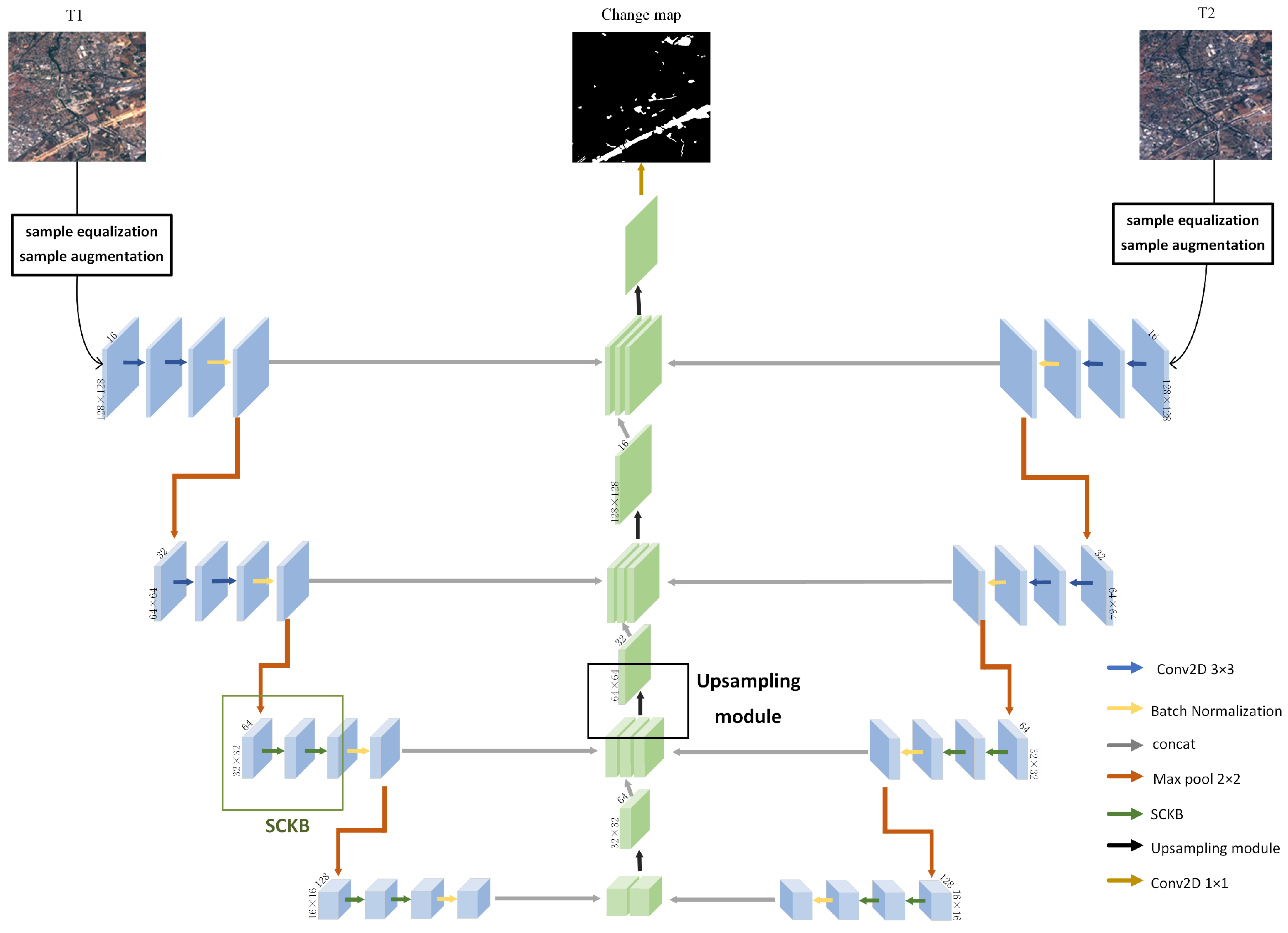
- A multispectral image change detection framework based on multi-scale adaptive kernel network (MSAK-Net) is designed, which is an encoder-decoder architecture. The framework extends the U-Net bilaterally and retains the jump connection. The encoding path effectively mines the multi-scale deep features in the original image. An attention mechanism is introduced into the decoding path to enhance the use of useful information. After that, the multimodal conditional random field is used to post-process the network results to refine the classification boundary.
- (2)
- A selective convolution kernel block (SCKB) is designed to fully exploit the complex spatial features in multispectral images. SCKB assigns an adaptive weight to the convolution branches of different scales to obtain better multi-scale features. In addition, the designed upsampling module is embedded in the decoding path, which uses the attention mechanism to integrate the change information and improve the use of the useful information of the task.
2. Methodology
2.1. The Framework of the Change Detection Algorithm
2.2. The Architecture of the MSAK-Net
2.3. Selective Convolution Kernel Block
2.4. Attention Module-Based Upsampling Unit
2.5. Secondary Classification Method Based on Multimodal Conditional Random Field
3. Experiment Settings
3.1. Datasets Description
3.2. Experimental Setup
3.3. Compared Methods
- •
- Fully Convolutional Siamese-Concatenation (FC-Siam-conc)This method belongs to a typical late fusion method proposed by Rodrigo et al. [27]. First, the siamese network is used to extract the high-dimensional features in the bi-temporal image, and then the bi-temporal high-dimensional features are superimposed in the channel dimension, and then input to the discriminator to detect the change features.
- •
- Fully Convolutional Siamese-Difference (FC-Siam-diff)This method is similar to the network structure of FC-Siam-conc, except that the input to the discriminator is the absolute value of the difference between two high-dimensional features.
- •
- U-NetThis method adopts the U-Net network structure for change detection, but considering the size of the input training samples, the network only contains four max pooling layers and four upsampling layers. Furthermore, the input data of the encoding path is spliced by early fusion.
- •
- Deep Siamese Multiscale Convolutional Network (DSMS-CN)The algorithm is proposed by Chen Wu et al. [32]. This is the first time that Inception module is exploited for Siamese neural network and four convolutional branches are used to extract deep features at different scales.
- •
- Densely connected siamese network (SNUNet)SNUNet, proposed by Fang et al. [38], is a combination of Siamese network and NestedUNet with its proposed ensemble channel attention module (ECAM) added to it for deep monitoring.
3.4. Evaluation Metrics
4. Results
4.1. Experimental Result and Analysis on the OSCD Dataset
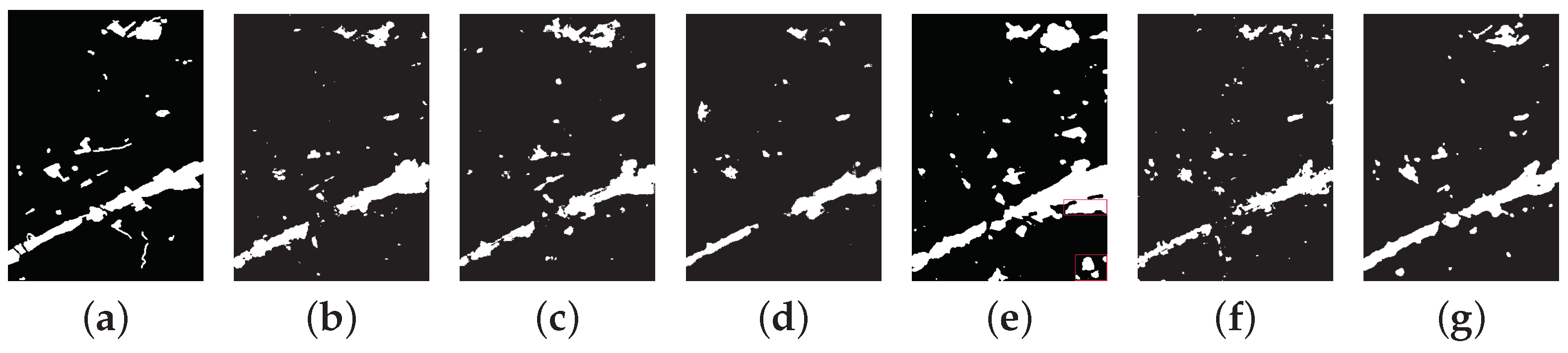
4.2. Experimental Result and Analysis on SZTAKI Dataset
5. Discussion
5.1. Ablation Study
5.2. Effect of Kernel Size in SCKB Module
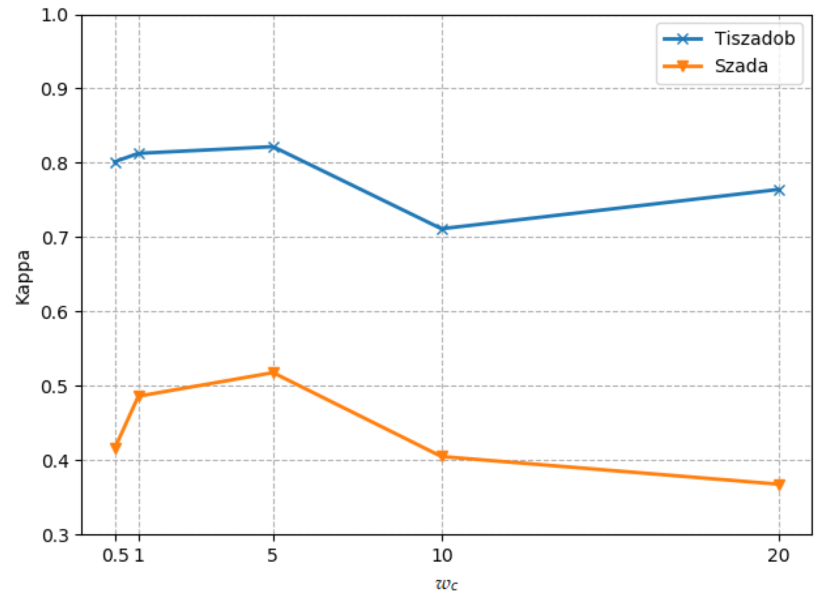
5.3. Effect of Class Weight
5.4. Computation Time Analysis
6. Conclusions
Author Contributions
Funding
Institutional Review Board Statement
Informed Consent Statement
Data Availability Statement
Conflicts of Interest
References
- Li, Y.; Peng, C.; Chen, Y.; Jiao, L.; Zhou, L.; Shang, R. A deep learning method for change detection in synthetic aperture radar images. IEEE Trans. Geosci. Remote Sens. 2019, 57, 5751–5763. [Google Scholar] [CrossRef]
- Zhang, W.; Lu, X. The Spectral-Spatial Joint Learning for Change Detection in Multispectral Imagery. Remote Sens. 2019, 11, 240. [Google Scholar] [CrossRef]
- Mou, L.; Bruzzone, L.; Zhu, X.X. Learning Spectral-Spatial-Temporal Features via a Recurrent Convolutional Neural Network for Change Detection in Multispectral Imagery. IEEE Trans. Geosci. Remote Sens. 2019, 57, 924–935. [Google Scholar] [CrossRef]
- He, Y.; Jia, Z.; Yang, J.; Kasabov, N.K. Multispectral Image Change Detection Based on Single-Band Slow Feature Analysis. Remote Sens. 2021, 13, 2969. [Google Scholar] [CrossRef]
- Shi, W.; Zhang, M.; Zhang, R.; Chen, S.; Zhan, Z. Change Detection Based on Artificial Intelligence: State-of-the-Art and Challenges. Remote Sens. 2020, 12, 1688. [Google Scholar] [CrossRef]
- Panuju, D.R.; Paull, D.J.; Griffin, A.L. Change Detection Techniques Based on Multispectral Images for Investigating Land Cover Dynamics. Remote Sens. 2020, 12, 1781. [Google Scholar] [CrossRef]
- Bovolo, F.; Bruzzone, L. A theoretical framework for unsupervised change detection based on change vector analysis in the polar domain. IEEE Trans. Geosci. Remote Sens. 2007, 45, 218–236. [Google Scholar] [CrossRef]
- Nielsen, A.A.; Conradsen, K.; Simpson, J.J. Multivariate alteration detection (MAD) and MAF postprocessing in multispectral, bitemporal image data: New approaches to change detection studies. Remote Sens. Environ. 1998, 64, 1–19. [Google Scholar] [CrossRef]
- Nielsen, A.A. The regularized iteratively reweighted MAD method for change detection in multi- and hyperspectral data. IEEE Trans. Image Process. 2007, 16, 463–478. [Google Scholar] [CrossRef] [PubMed]
- Wu, C.; Du, B.; Zhang, L. Slow Feature Analysis for Change Detection in Multispectral Imagery. IEEE Trans. Geosci. Remote Sens. 2014, 52, 2858–2874. [Google Scholar] [CrossRef]
- Bruzzone, L.; Prieto, D.F. An MRF approach to unsupervised change detection. In Proceedings of the 1999 International Conference on Image Processing (Cat. 99CH36348), Kobe, Japan, 24–28 October 1999; Volume 1, pp. 143–147. [Google Scholar]
- Lv, P.; Zhong, Y.; Zhao, J.; Zhang, L. Unsupervised change detection based on hybrid conditional random field model for high spatial resolution remote sensing imagery. IEEE Trans. Geosci. Remote Sens. 2018, 56, 4002–4015. [Google Scholar] [CrossRef]
- Hoberg, T.; Rottensteiner, F.; Feitosa, R.Q.; Heipke, C. Conditional random fields for multitemporal and multiscale classification of optical satellite imagery. IEEE Trans. Geosci. Remote Sens. 2014, 53, 659–673. [Google Scholar] [CrossRef]
- Zhao, J.; Zhong, Y.; Shu, H.; Zhang, L. High-resolution image classification integrating spectral-spatial-location cues by conditional random fields. IEEE Trans. Image Process. 2016, 25, 4033–4045. [Google Scholar] [CrossRef] [PubMed]
- Zhang, B.; Wang, C.; Shen, Y.; Liu, Y. Fully Connected Conditional Random Fields for High-Resolution Remote Sensing Land Use/Land Cover Classification with Convolutional Neural Networks. Remote Sens. 2018, 10, 1889. [Google Scholar] [CrossRef]
- Krähenbühl, P.; Koltun, V. Efficient Inference in Fully Connected CRFs with Gaussian Edge Potentials. In Proceedings of the 24th International Conference on Neural Information Processing Systems, Granada, Spain, 12–15 December 2011; pp. 109–117. [Google Scholar]
- Saha, S.; Solano-Correa, Y.T.; Bovolo, F.; Bruzzone, L. Unsupervised Deep Transfer Learning-Based Change Detection for HR Multispectral Images. IEEE Geosci. Remote Sens. Lett. 2021, 18, 856–860. [Google Scholar] [CrossRef]
- Shafique, A.; Cao, G.; Khan, Z.; Asad, M.; Aslam, M. Deep learning-based change detection in remote sensing images: A review. Remote Sens. 2022, 14, 871. [Google Scholar] [CrossRef]
- Liu, S.; Bruzzone, L.; Bovolo, F.; Du, P. Hierarchical unsupervised change detection in multitemporal hyperspectral images. IEEE Trans. Geosci. Remote Sens. 2014, 53, 244–260. [Google Scholar]
- Ferraris, V.; Dobigeon, N.; Wei, Q.; Chabert, M. Detecting changes between optical images of different spatial and spectral resolutions: A fusion-based approach. IEEE Trans. Geosci. Remote Sens. 2017, 56, 1566–1578. [Google Scholar] [CrossRef]
- Lin, Y.; Li, S.; Fang, L.; Ghamisi, P. Multispectral Change Detection With Bilinear Convolutional Neural Networks. IEEE Geosci. Remote Sens. Lett. 2020, 17, 1757–1761. [Google Scholar] [CrossRef]
- Tan, K.; Zhang, Y.; Wang, X.; Chen, Y. Object-Based Change Detection Using Multiple Classifiers and Multi-Scale Uncertainty Analysis. Remote Sens. 2019, 11, 359. [Google Scholar] [CrossRef]
- Zhang, C.; Yue, P.; Tapete, D.; Shangguan, B.; Wang, M.; Wu, Z. A multi-level context-guided classification method with object-based convolutional neural network for land cover classification using very high resolution remote sensing images. Int. J. Appl. Earth Obs. Geoinf. 2020, 88, 102086. [Google Scholar] [CrossRef]
- Sun, S.; Mu, L.; Wang, L.; Liu, P. L-UNet: An LSTM Network for Remote Sensing Image Change Detection. IEEE Geosci. Remote Sens. Lett. 2022, 19, 1–5. [Google Scholar] [CrossRef]
- Peng, D.; Bruzzone, L.; Zhang, Y.; Guan, H.; Ding, H.; Huang, X. SemiCDNet: A Semisupervised Convolutional Neural Network for Change Detection in High Resolution Remote-Sensing Images. IEEE Trans. Geosci. Remote Sens. 2021, 59, 5891–5906. [Google Scholar] [CrossRef]
- Ji, S.; Wei, S.; Lu, M. Fully Convolutional Networks for Multisource Building Extraction From an Open Aerial and Satellite Imagery Data Set. IEEE Trans. Geosci. Remote Sens. 2019, 57, 574–586. [Google Scholar] [CrossRef]
- Daudt, R.C.; Le Saux, B.; Boulch, A. Fully convolutional siamese networks for change detection. In Proceedings of the 2018 25th IEEE International Conference on Image Processing (ICIP), Athens, Greece, 7–10 October 2018; pp. 4063–4067. [Google Scholar]
- Chen, H.; Wu, C.; Du, B.; Zhang, L.; Wang, L. Change Detection in Multisource VHR Images via Deep Siamese Convolutional Multiple-Layers Recurrent Neural Network. IEEE Trans. Geosci. Remote Sens. 2020, 58, 2848–2864. [Google Scholar] [CrossRef]
- Kusetogullari, H.; Yavariabdi, A.; Celik, T. Unsupervised change detection in multitemporal multispectral satellite images using parallel particle swarm optimization. IEEE J. Sel. Top. Appl. Earth Obs. Remote Sens. 2015, 8, 2151–2164. [Google Scholar] [CrossRef]
- Hou, B.; Wang, Y.; Liu, Q. Change Detection Based on Deep Features and Low Rank. IEEE Geosci. Remote Sens. Lett. 2017, 14, 2418–2422. [Google Scholar] [CrossRef]
- Liu, T.; Yang, L.; Lunga, D. Change detection using deep learning approach with object-based image analysis. Remote Sens. Environ. 2021, 256, 112308. [Google Scholar] [CrossRef]
- Chen, H.; Wu, C.; Du, B.; Zhang, L. Deep Siamese Multi-scale Convolutional Network for Change Detection in Multi-temporal VHR Images. In Proceedings of the 2019 10th International Workshop on the Analysis of Multitemporal Remote Sensing Images (Multitemp), Shanghai, China, 5–7 August 2019. [Google Scholar]
- Song, A.; Choi, J. Fully convolutional networks with multiscale 3D filters and transfer learning for change detection in high spatial resolution satellite images. Remote Sens. 2020, 12, 799. [Google Scholar] [CrossRef]
- Zhang, X.; He, L.; Qin, K.; Dang, Q.; Si, H.; Tang, X.; Jiao, L. SMD-Net: Siamese Multi-Scale Difference-Enhancement Network for Change Detection in Remote Sensing. Remote Sens. 2022, 14, 1580. [Google Scholar] [CrossRef]
- Mnih, V.; Heess, N.; Graves, A. Recurrent models of visual attention. In Proceedings of the 27th International Conference on Neural Information Processing Systems-Volume 2, Montreal, Canada, 8–13 December 2014; pp. 2204–2212. [Google Scholar]
- Zhang, C.; Yue, P.; Tapete, D.; Jiang, L.; Shangguan, B.; Huang, L.; Liu, G. A deeply supervised image fusion network for change detection in high resolution bi-temporal remote sensing images. ISPRS J. Photogramm. Remote Sens. 2020, 166, 183–200. [Google Scholar] [CrossRef]
- Peng, X.; Zhong, R.; Li, Z.; Li, Q. Optical Remote Sensing Image Change Detection Based on Attention Mechanism and Image Difference. IEEE Trans. Geosci. Remote Sens. 2021, 59, 7296–7307. [Google Scholar] [CrossRef]
- Fang, S.; Li, K.; Shao, J.; Li, Z. SNUNet-CD: A densely connected Siamese network for change detection of VHR images. IEEE Geosci. Remote Sens. Lett. 2021, 19, 1–5. [Google Scholar] [CrossRef]
- Chen, H.; Shi, Z. A Spatial-Temporal Attention-Based Method and a New Dataset for Remote Sensing Image Change Detection. Remote Sens. 2020, 12, 1662. [Google Scholar] [CrossRef]
- Woo, S.; Park, J.; Lee, J.Y.; Kweon, I.S. Cbam: Convolutional block attention module. In Proceedings of the European Conference on Computer Vision (ECCV), Munich, Germany, 8–14 September 2018; pp. 3–19. [Google Scholar]
- Szegedy, C.; Liu, W.; Jia, Y.; Sermanet, P.; Reed, S.; Anguelov, D.; Erhan, D.; Vanhoucke, V.; Rabinovich, A. Going Deeper with Convolutions. In Proceedings of the 2015 IEEE Conference on Computer Vision and Pattern Recognition (CVPR), Boston, MA, USA, 7–12 June 2015; pp. 1–9. [Google Scholar] [CrossRef]
- Zhang, Z.; Liu, Q.; Wang, Y. Road Extraction by Deep Residual U-Net. IEEE Geosci. Remote Sens. Lett. 2018, 15, 749–753. [Google Scholar] [CrossRef]
- Shi, C.; Zhou, Y.; Qiu, B.; Guo, D.; Li, M. CloudU-Net: A Deep Convolutional Neural Network Architecture for Daytime and Nighttime Cloud Images’ Segmentation. IEEE Geosci. Remote Sens. Lett. 2021, 18, 1688–1692. [Google Scholar] [CrossRef]
- Feng, W.; Sui, H.; Huang, W.; Xu, C.; An, K. Water Body Extraction From Very High-Resolution Remote Sensing Imagery Using Deep U-Net and a Superpixel-Based Conditional Random Field Model. IEEE Geosci. Remote Sens. Lett. 2019, 16, 618–622. [Google Scholar] [CrossRef]
- Shi, W.; Zhang, M.; Ke, H.; Fang, X.; Zhan, Z.; Chen, S. Landslide Recognition by Deep Convolutional Neural Network and Change Detection. IEEE Trans. Geosci. Remote Sens. 2021, 59, 4654–4672. [Google Scholar] [CrossRef]
- Jiang, H.; Peng, M.; Zhong, Y.; Xie, H.; Hao, Z.; Lin, J.; Ma, X.; Hu, X. A Survey on Deep Learning-Based Change Detection from High-Resolution Remote Sensing Images. Remote Sens. 2022, 14, 1552. [Google Scholar] [CrossRef]


| Test Set | Metric | FC-Siam-Conc | FC-Siam-Diff | U-Net | DSMS-CN | SNUNet | MSAK-Net-MCRF |
|---|---|---|---|---|---|---|---|
| Montpellier | Precision | 0.7476 | 0.7375 | 0.8438 | 0.5070 | 0.7895 | 0.7482 |
| Recall | 0.6503 | 0.6895 | 0.5422 | 0.7694 | 0.5991 | 0.7751 | |
| Acc | 0.9506 | 0.9518 | 0.9516 | 0.9131 | 0.9514 | 0.9593 | |
| F1 | 0.6956 | 0.7127 | 0.6602 | 0.6112 | 0.6813 | 0.7614 | |
| Kappa | 0.6689 | 0.6865 | 0.6355 | 0.5658 | 0.6555 | 0.7392 | |
| Lasvegas | Precision | 0.6619 | 0.6822 | 0.7198 | 0.6388 | 0.7586 | 0.7689 |
| Recall | 0.4584 | 0.6582 | 0.2610 | 0.7983 | 0.5369 | 0.6624 | |
| Acc | 0.9356 | 0.9464 | 0.9305 | 0.9460 | 0.9476 | 0.9556 | |
| F1 | 0.5417 | 0.6700 | 0.3831 | 0.7097 | 0.6288 | 0.7117 | |
| Kappa | 0.5084 | 0.6409 | 0.3546 | 0.6804 | 0.6015 | 0.6879 |
| Test set | Metric | FC-Siam-Conc | FC-Siam-Diff | U-Net | DSMS-CN | SNUNet | MSAK-Net-MCRF |
|---|---|---|---|---|---|---|---|
| Tiszadob | Precision | 0.9428 | 0.7416 | 0.8933 | 0.7712 | 0.8607 | 0.7491 |
| Recall | 0.7392 | 0.6869 | 0.6848 | 0.7955 | 0.7087 | 0.9920 | |
| Acc | 0.9476 | 0.9319 | 0.9319 | 0.9235 | 0.9438 | 0.9409 | |
| F1 | 0.8287 | 0.7758 | 0.7753 | 0.7832 | 0.7773 | 0.8536 | |
| Kappa | 0.7983 | 0.7365 | 0.7360 | 0.7367 | 0.7455 | 0.8175 | |
| Szada | Precision | 0.4316 | 0.4760 | 0.3709 | 0.4636 | 0.3688 | 0.5715 |
| Recall | 0.4029 | 0.4602 | 0.3779 | 0.6048 | 0.4759 | 0.5139 | |
| Acc | 0.9409 | 0.9452 | 0.9477 | 0.9426 | 0.9624 | 0.9554 | |
| F1 | 0.4168 | 0.4680 | 0.3744 | 0.5249 | 0.4156 | 0.5412 | |
| Kappa | 0.3858 | 0.4391 | 0.3584 | 0.4949 | 0.3965 | 0.5172 |
| Test Set | Method | F1 | Kappa |
|---|---|---|---|
| Montpellier of OSCD dataset | MSAK-Net | 0.7599 | 0.7370 |
| MSAK-Net-MCRF | 0.7614 | 0.7392 | |
| Lasvegas of OSCD dataset | MSAK-Net | 0.7100 | 0.6856 |
| MSAK-Net-MCRF | 0.7117 | 0.6879 | |
| Tiszadob of SZTAKI dataset | MSAK-Net | 0.8514 | 0.8147 |
| MSAK-Net-MCRF | 0.8536 | 0.8175 | |
| Szada of SZTAKI dataset | MSAK-Net | 0.5407 | 0.5166 |
| MSAK-Net-MCRF | 0.5412 | 0.5172 |
| Kappa | ||||||
|---|---|---|---|---|---|---|
| 0 | 0.5 | 1 | 2 | 3 | ||
| 0 | 0.8147 | 0.8155 | 0.8164 | 0.8175 | 0.8183 | |
| 0.5 | 0.8155 | 0.8164 | 0.8172 | 0.8179 | 0.8189 | |
| 1 | 0.8164 | 0.8172 | 0.8175 | 0.8184 | 0.8188 | |
| 2 | 0.8175 | 0.8179 | 0.8183 | 0.8188 | 0.8177 | |
| 3 | 0.8183 | 0.8189 | 0.8188 | 0.8177 | 0.8161 | |
| Method | F1 | Kappa |
|---|---|---|
| MSAK-Net | 0.8514 | 0.8147 |
| MSAK-Net without SCKB | 0.8306 | 0.7888 |
| MSAK-Net without attention mechanism | 0.8489 | 0.8129 |
| Method | Training Time (s/epoch) | Testing Time (s) |
|---|---|---|
| FC-Siam-conc | 45.97 | 0.27 |
| FC-Siam-diff | 47.27 | 0.18 |
| U-Net | 55.98 | 0.40 |
| DSMS-CN | 42.08 | 5.84 |
| SNUNet | 62.60 | 1.73 |
| MSAK-Net-MCRF | 50.11 | 6.97 |
Publisher’s Note: MDPI stays neutral with regard to jurisdictional claims in published maps and institutional affiliations. |
© 2022 by the authors. Licensee MDPI, Basel, Switzerland. This article is an open access article distributed under the terms and conditions of the Creative Commons Attribution (CC BY) license (https://creativecommons.org/licenses/by/4.0/).
Share and Cite
Feng, S.; Fan, Y.; Tang, Y.; Cheng, H.; Zhao, C.; Zhu, Y.; Cheng, C. A Change Detection Method Based on Multi-Scale Adaptive Convolution Kernel Network and Multimodal Conditional Random Field for Multi-Temporal Multispectral Images. Remote Sens. 2022, 14, 5368. https://doi.org/10.3390/rs14215368
Feng S, Fan Y, Tang Y, Cheng H, Zhao C, Zhu Y, Cheng C. A Change Detection Method Based on Multi-Scale Adaptive Convolution Kernel Network and Multimodal Conditional Random Field for Multi-Temporal Multispectral Images. Remote Sensing. 2022; 14(21):5368. https://doi.org/10.3390/rs14215368
Chicago/Turabian StyleFeng, Shou, Yuanze Fan, Yingjie Tang, Hao Cheng, Chunhui Zhao, Yaoxuan Zhu, and Chunhua Cheng. 2022. "A Change Detection Method Based on Multi-Scale Adaptive Convolution Kernel Network and Multimodal Conditional Random Field for Multi-Temporal Multispectral Images" Remote Sensing 14, no. 21: 5368. https://doi.org/10.3390/rs14215368
APA StyleFeng, S., Fan, Y., Tang, Y., Cheng, H., Zhao, C., Zhu, Y., & Cheng, C. (2022). A Change Detection Method Based on Multi-Scale Adaptive Convolution Kernel Network and Multimodal Conditional Random Field for Multi-Temporal Multispectral Images. Remote Sensing, 14(21), 5368. https://doi.org/10.3390/rs14215368