

A Robust and Effective Identification Method for Point-Distributed Coded Targets in Digital Close-Range Photogrammetry

 ,
,  , and
, and
Abstract
:
1. Introduction
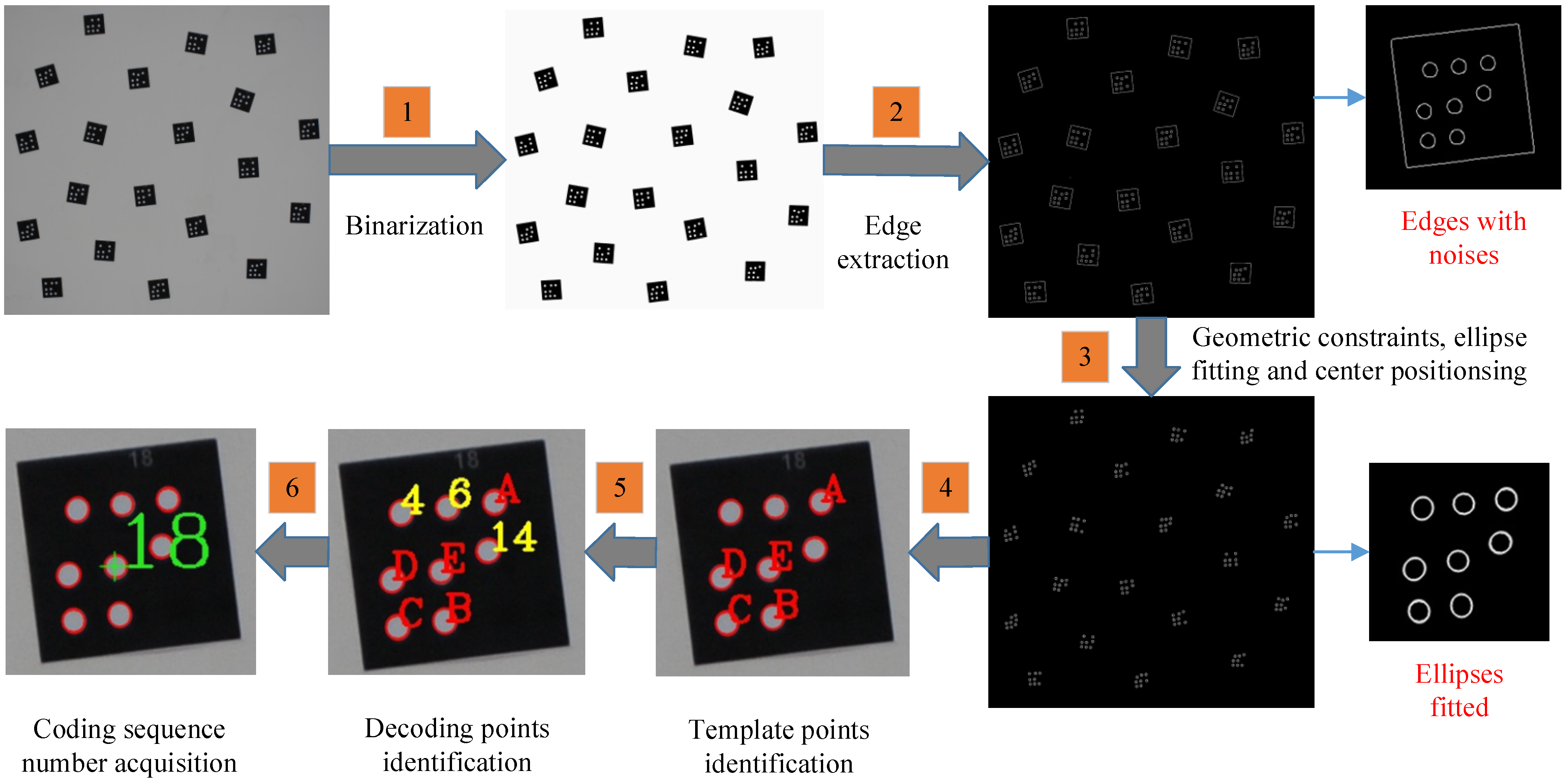
2. Methods
2.1. Construction of GCTs
2.2. Identification of Template Points
2.2.1. P2-Invariant of Four Collinear Points
2.2.2. P2-Invariant of Five Coplanar Points
2.2.3. Identification of Template Points under Collinear Condition
2.3. Decoding
2.4. Identification Process of GCTs
- (1)
- Geometric Constraints
- (2)
- Center Positioning of Points
- (3)
- Point-set Search
- Find three collinear points among the eight points, and then check the remaining five points. Make sure that three points are on one side of the line formed by these three collinear points and that the other two points are on the other side.
- Choose a point separately from either side of the line, which together with the three collinear points form five coplanar points to construct P2-invariant. Except for the three collinear points, two of the remaining five points are selected to join with the three collinear points to construct template points. The two points are constrained by the geometric restricted condition , where is the distance from the positioning point E to D or B. The applicable value of is 2.5.
3. Results
3.1. Experiment for Indoor Scenes
- (1)
- Experiments with Increasing Step of Viewing Angles
- (2)
- Experiments with Small GCTs
- (3)
- Experiments with mixed GCTs
3.2. Experiment for Outdoor Scenes
3.3. Experiment for UAV
4. Discussion
4.1. The P2-Invariant of Template Points
4.2. The Identification Positioning Bias of Decoding Points
4.3. The Precision of Center Positioning of GCTs
5. Conclusions
Author Contributions
Funding
Institutional Review Board Statement
Informed Consent Statement
Data Availability Statement
Conflicts of Interest
References
- Tushev, S.; Sukhovilov, B.; Sartasov, E. Architecture of industrial close-range photogrammetric system with multi-functional coded targets. In Proceedings of the 2nd International Ural Conference on Measurements (UralCon), Chelyabinsk, Russia, 16–19 October 2017; pp. 435–442. [Google Scholar] [CrossRef]
- Burger, W.; Burge, M.J. Scale-invariant feature transform (SIFT). In Digital Image Processing; Springer: Cham, Switzerland, 2022; pp. 709–763. [Google Scholar]
- Yang, B.; Qin, L.; Liu, J.; Liu, X. UTRNet: An Unsupervised Time-Distance-Guided Convolutional Recurrent Network for Change Detection in Irregularly Collected Images. IEEE Trans. Geosci. Remote Sens. 2022, 60, 4410516. [Google Scholar] [CrossRef]
- Dai, X.; Cheng, J.; Gao, Y.; Guo, S.; Yang, X.; Xu, X.; Cen, Y. Deep belief network for feature extraction of urban artificial targets. Math. Probl. Eng. 2020, 2020, 2387823. [Google Scholar] [CrossRef]
- Wang, Y.M.; Yu, S.Y.; Ren, S.; Cheng, S.; Liu, J.Z. Close-range industrial photogrammetry and application: Review and outlook. In Proceedings of the AOPC 2020: Optics Ultra Precision Manufacturing and Testing, Beijing, China, 30 November–2 December 2020; Volume 11568, pp. 152–162. [Google Scholar]
- Barbero-García, I.; Cabrelles, M.; Lerma, J.L.; Marqués-Mateu, Á. Smartphone-based close-range photogrammetric assessment of spherical objects. Photogramm. Rec. 2018, 33, 283–299. [Google Scholar] [CrossRef] [Green Version]
- Wang, M.; Guo, Y.; Wang, Q.; Liu, Y.; Liu, J.; Song, X.; Wang, G.; Zhang, H. A Novel Capacity Expansion and Recognition Acceleration Method for Dot-dispersing Coded Targets in Photogrammetry. Meas. Sci. Technol. 2022, 33, 125016. [Google Scholar] [CrossRef]
- Shi, Y.; Zhang, L. Design of Chinese character coded targets for feature point recognition under motion-blur effect. IEEE Access 2020, 8, 124467–124475. [Google Scholar] [CrossRef]
- Mohammadi, M.; Rashidi, M.; Mousavi, V.; Yu, Y.; Samali, B. Application of TLS Method in Digitization of Bridge Infrastructures: A Path to BrIM Development. Remote Sens. 2022, 14, 1148. [Google Scholar] [CrossRef]
- Mohammadi, M.; Rashidi, M.; Mousavi, V.; Karami, A.; Yu, Y.; Samali, B. Quality Evaluation of Digital Twins Generated Based on UAV Photogrammetry and TLS: Bridge Case Study. Remote Sens. 2021, 13, 3499. [Google Scholar] [CrossRef]
- Mohammadi, M.; Rashidi, M.; Mousavi, V.; Karami, A.; Yu, Y.; Samali, B. Case study on accuracy comparison of digital twins developed for a heritage bridge via UAV photogrammetry and terrestrial laser scanning. In Proceedings of the 10th International Conference on Structural Health Monitoring of Intelligent Infrastructure, SHMII, Porto, Portugal, 30 June–2 July 2021; Volume 10. [Google Scholar]
- Yang, X.; Fang, S.; Kong, B.; Li, Y. Design of a color coded target for vision measurements. Optik 2014, 125, 3727–3732. [Google Scholar] [CrossRef]
- Karimi, M.; Zakariyaeinejad, Z.; Sadeghi-Niaraki, A.; Ahmadabadian, A.H. A new method for automatic and accurate coded target recognition in oblique images to improve augmented reality precision. Trans. GIS 2022, 26, 1509–1530. [Google Scholar] [CrossRef]
- Xia, X.; Zhang, X.; Fayek, S.; Yin, Z. A table method for coded target decoding with application to 3-D reconstruction of soil specimens during triaxial testing. Acta Geotech. 2021, 16, 3779–3791. [Google Scholar] [CrossRef]
- Hurník, J.; Zatočilová, A.; Paloušek, D. Circular coded target system for industrial applications. Mach. Vis. Appl. 2021, 32, 39. [Google Scholar] [CrossRef]
- Mousavi, V.; Khosravi, M.; Ahmadi, M.; Noori, N.; Haghshenas, S.; Hosseininaveh, A.; Varshosaz, M. The performance evaluation of multi-image 3D reconstruction software with different sensors. Measurement 2018, 120, 1–10. [Google Scholar] [CrossRef]
- Novosad, M. Lidar Pose Calibration Using Coded Reflectance Targets. Bachelor’s Thesis, Faculty of Electrical Engineering, Czech Technical University in Prague, Prague, Czech Republic, 2021. [Google Scholar]
- Shortis, M.R.; Seager, J.W. A practical target recognition system for close range photogrammetry. Photogramm. Rec. 2014, 29, 337–355. [Google Scholar] [CrossRef]
- Sukhovilov, B.M.; Sartasov, E.M.; Grigorova, E.A. Improving the accuracy of determining the position of the code marks in the problems of constructing three-dimensional models of objects. In Proceedings of the 2nd International Conference on Industrial Engineering, Chelyabinsk, Russia, 19–20 May 2016; pp. 19–20. [Google Scholar] [CrossRef]
- Tushev, S.; Sukhovilov, B.; Sartasov, E. Robust coded target recognition in adverse light conditions. In Proceedings of the 2018 International Conference on Industrial Engineering, Applications and Manufacturing (ICIEAM), Moscow, Russia, 15–18 May 2018; IEEE: Piscataway, NJ, USA, 2018; pp. 1–6. [Google Scholar]
- Yan, X.; Deng, H.; Quan, Q. Active Infrared Coded Target Design and Pose Estimation for Multiple Objects. In Proceedings of the 2019 IEEE/RSJ International Conference on Intelligent Robots and Systems (IROS), Macau, China, 4–8 November 2019; pp. 6885–6890. [Google Scholar] [CrossRef]
- Kniaz, V.V.; Grodzitskiy, L.; Knyaz, V.A. Deep learning for coded target detection. Int. Arch. Photogramm. Remote Sens. Spat. Inf. Sci. 2021, 4421, 125–130. [Google Scholar] [CrossRef]
- Schneider, C.T.; Sinnreich, K. Optical 3-D measurement systems for quality control in industry. Int. Arch. Photogramm. Remote Sens. 1993, 29, 56–59. Available online: www.isprs.org/proceedings/xxix/congress/part5/56_xxix-part5.pdf (accessed on 26 June 2022).
- Hattori, S.; Akimoto, K.; Fraser, C.; Imoto, H. Automated procedures with coded targets in industrial vision metrology. Photogramm. Eng. Remote Sens. 2002, 68, 441–446. Available online: www.asprs.org/wp-content/uploads/pers/2002journal/may/2002_may_441-446.pdf (accessed on 25 June 2022).
- Fraser, C.S. Innovations in automation for vision metrology systems. Photogramm. Rec. 1997, 15, 901–911. [Google Scholar] [CrossRef]
- Brown, J.D.; Dold, J. V-STARS—A system for digital industrial photogrammetry. In Optical 3-D Measurement Techniques III; Gruen, A., Kahmen, H., Eds.; Wichmann Verlag: Heidelberg, Germany, 1995; pp. 12–21. [Google Scholar]
- Fraser, C.S.; Edmundson, K.L. Design and implementation of a computational processing system for off-line digital close-range photogrammetry. ISPRS J. Photogramm. Remote Sens. 2000, 55, 94–104. [Google Scholar] [CrossRef]
- Al-Kharaz, A.A.; Chong, A. Reliability of a close-range photogrammetry technique to measure ankle kinematics during active range of motion in place. Foot 2021, 46, 101763. [Google Scholar] [CrossRef]
- Filion, A.; Joubair, A.; Tahan, A.S.; Bonev, I.A. Robot calibration using a portable photogrammetry system. Robot. Comput.-Integr. Manuf. 2018, 49, 77–87. [Google Scholar] [CrossRef]
- Hattori, S.; Akimoto, K.; Ohnishi, Y.; Miura, S. Semi-automated tunnel measurement by vision metrology using coded-targets. In Modern Tunneling Science and Technology, 1st ed.; Adachi, T., Tateyama, K., Kimura, M., Eds.; Routledge: London, UK, 2017; pp. 285–288. [Google Scholar]
- Zou, J.; Meng, L. Design of a New Coded Target with Large Coding Capacity for Close—Range Photogrammetry and Research on Recognition Algorithm. IEEE Access 2020, 8, 220285–220292. [Google Scholar] [CrossRef]
- Brown, J. V-STARS/S Acceptance Test Results. In: Seattle: Boeing Large Scale Optical Metrology Seminar. 1998. Available online: http://gancell.com/papers/S%20Acceptance%20Test%20Results%20-%20metric%20version.pdf (accessed on 25 August 2022).
- Hartley, R.; Zisserman, A. Multiple View Geometry in Computer Vision; Cambridge University Press: Cambridge, UK, 2003. [Google Scholar]
- Yuan, S.; Bi, D.; Li, Z.; Yan, N.; Zhang, X. A static and fast calibration method for line scan camera based on cross-ratio invariance. J. Mod. Opt. 2022, 69, 619–627. [Google Scholar] [CrossRef]
- Su, D.; Bender, A.; Sukkarieh, S. Improved cross-ratio invariant-based intrinsic calibration of a hyperspectral line-scan camera. Sensors 2018, 18, 1885. [Google Scholar] [CrossRef] [PubMed] [Green Version]
- Lei, G. Recognition of planar objects in 3-D space from single perspective views using cross-ratio. IEEE Trans. Robot. Autom. 1990, 6, 432–437. [Google Scholar] [CrossRef]
- Meer, P.; Ramakrishna, S.; Lenz, R. Correspondence of coplanar features through p2-invariant representations. In Proceedings of the Joint European-US Workshop on Applications of Invariance in Computer Vision, Ponta Delgada, Portugal, 9–14 October 1993; Springer: Berlin/Heidelberg, Germany, 1993; pp. 473–492. [Google Scholar]
- Bergamasco, F.; Albarelli, A.; Torsello, A. Pi-tag: A fast image-space marker design based on projective invariants. Mach. Vis. Appl. 2013, 24, 1295–1310. Available online: https://link.springer.com/article/10.1007/s00138-012-0469-6 (accessed on 25 September 2022). [CrossRef] [Green Version]
- Cha, J.; Kim, G. Camera motion parameter estimation technique using 2D homography and LM method based on projective and permutation invariant features. In Proceedings of the International Conference on Computational Science and Its Applications, Glasgow, UK, 8–11 May 2006; Springer: Berlin/Heidelberg, Germany, 2006; pp. 432–440. [Google Scholar]
- Min, C.; Gu, Y.; Li, Y.; Yang, F. Non-rigid infrared and visible image registration by enhanced affine transformation. Pattern Recognit. 2020, 106, 107377. [Google Scholar] [CrossRef]
- Kaehler, A. Learning OpenCV Computer Vision in C++ with the OpenCV Library Early Release; O’Relly: Springfield, MO, USA, 2013; p. 575. [Google Scholar]
- Wang, W.; Pang, Y.; Ahmat, Y.; Liu, Y.; Chen, A. A novel cross-circular coded target for photogrammetry. Optik 2021, 244, 167517. [Google Scholar] [CrossRef]
- Why V-STARS? Available online: https://www.geodetic.com/v-stars/ (accessed on 27 August 2022).
- Kanatani, K.; Sugaya, Y.; Kanazawa, Y. Ellipse fitting for computer vision: Implementation and applications. Synth. Lect. Comput. Vis. 2016, 6, 1–141. [Google Scholar]
- Setan, H.; Ibrahim, M.S. High Precision Digital Close Range Photogrammetric System for Industrial Application Using V-STARS: Some Preliminary Result. In Proceedings of the International Geoinformation Symposium, Bogotá, Colombia, 24–26 September 2003. [Google Scholar]
- Liu, Y.; Su, X.; Guo, X.; Suo, T.; Yu, Q. A Novel Concentric Circular Coded Target, and Its Positioning and Identifying Method for Vision Measurement under Challenging Conditions. Sensors 2021, 21, 855. [Google Scholar] [CrossRef] [PubMed]
- Michalak, H.; Okarma, K. Adaptive image binarization based on multi-layered stack of regions. In Proceedings of the International Conference on Computer Analysis of Images and Patterns, Salerno, Italy, 2–5 September 2019; Springer: Cham, Switzerland, 2019; pp. 281–293. [Google Scholar]
- Dong, S.; Ma, J.; Su, Z.; Li, C. Robust circular marker localization under non-uniform illuminations based on homomorphic filtering. Measurement 2021, 170, 108700. [Google Scholar] [CrossRef]
- Jia, Q.; Fan, X.; Luo, Z.; Song, L.; Qiu, T. A fast ellipse detector using projective invariant pruning. IEEE Trans. Image Process. 2017, 26, 3665–3679. [Google Scholar] [CrossRef]
- Michalak, H.; Okarma, K. Fast adaptive image binarization using the region based approach. In Proceedings of the Computer Science On-line Conference, Vsetin, Czech Republic, 25–28 April 2018; Springer: Cham, Switzerland, 2018; pp. 79–90. [Google Scholar]


| Point Type | Point Number | Coordinate Values/mm | Point Type | Point Number | Coordinate Values/mm | ||
|---|---|---|---|---|---|---|---|
| Template Points | A | 26 | 26 | Coding/Decoding Points | 12 | 26 | 11 |
| B | 11 | 0 | 13 | 26 | 15 | ||
| C | 0 | 0 | 15 | 23 | 15 | ||
| D | 0 | 11 | 16 | 23 | 11 | ||
| E | 11.5 | 11.5 | 17 | 11 | 23 | ||
| Coding/Decoding Points | 1 | 0 | 22 | 18 | 22 | 7.5 | |
| 2 | 0 | 26 | 19 | 26 | 7.5 | ||
| 3 | 4 | 22 | 20 | 7.5 | 26 | ||
| 4 | 4 | 26 | 21 | 15 | 30 | ||
| 5 | 11 | 26 | 22 | 11 | 30 | ||
| 6 | 15 | 26 | 23 | 4 | 30 | ||
| 7 | 15 | 23 | 24 | 0 | 30 | ||
| 8 | 22 | 0 | 25 | 30 | 15 | ||
| 9 | 26 | 0 | 26 | 30 | 11 | ||
| 10 | 22 | 4 | 27 | 30 | 4 | ||
| 11 | 26 | 4 | 28 | 30 | 0 | ||
| Decoding Serial Number | Numbers of Decoding Points | Decoding Value |
|---|---|---|
| CODE1 | 3, 6, 8 | 328 |
| CODE2 | 1, 7, 8 | 386 |
| … | … | |
| CODE18 | 4, 6, 14 | 16,464 |
| … | … | |
| CODE505 | 7, 17, 28 | 268,566,656 |
| Name of Point Target | Image Coordinates/px | Designed Coordinates/mm | ||
|---|---|---|---|---|
| A | 2047.00 | 1072.58 | 26 | 26 |
| B | 2326.77 | 1133.63 | 11 | 0 |
| C | 2331.21 | 1170.83 | 0 | 0 |
| D | 2368.04 | 1166.33 | 0 | 11 |
| E | 2364.86 | 1127.35 | 11.5 | 11.5 |
| I | 2333.77 | 1081.33 | - | - |
| II | 2370.47 | 1076.75 | - | - |
| III | 2401.81 | 1110.59 | - | - |
| a | b | c | d | e | f |
|---|---|---|---|---|---|
| −0.035 | −0.292 | 423.896 | 0.296 | −0.037 | −646.310 |
| Decoding Points | Transformed Coordinates | Designed Coordinates | Positioning Bias | Point Number | |||
|---|---|---|---|---|---|---|---|
| ∆x | ∆y | ||||||
| I | 4.011 | 26.025 | 4 | 26 | 0.011 | 0.025 | 4 |
| II | 15.032 | 26.070 | 15 | 26 | 0.032 | 0.070 | 6 |
| III | 23.056 | 15.088 | 23 | 15 | 0.056 | 0.088 | 14 |
| Area S/px | Perimeter C/px | Roundness K |
|---|---|---|
| 30~1000 | 20~500 | 0.6~1.0 |
| Viewing Angles | 0° | 10° | 20° | 30° | 40° | 50° | 60° | 65° | 70° | 75° | 80° |
|---|---|---|---|---|---|---|---|---|---|---|---|
| P2-Invariant Range | 2.447 ~ 2.536 | 2.458 ~ 2.509 | 2.467 ~ 2.532 | 2.465 ~ 2.515 | 2.444 ~ 2.552 | 2.442 ~ 2.527 | 2.461 ~ 2.573 | 2.450 ~ 2.587 | 2.430 ~ 2.555 | 2.401 ~ 2.468 | NaN |
| Mean Values | 2.493 | 2.485 | 2.492 | 2.489 | 2.487 | 2.492 | 2.500 | 2.501 | 2.503 | 2.435 | NaN |
| ∆ P2_RMS | 0.022 | 0.014 | 0.016 | 0.014 | 0.028 | 0.023 | 0.033 | 0.031 | 0.036 | 0.048 | NaN |
| Coding Serial Number | Center Positioning Coordinate (x, y) (Unit: px) | Positioning Bias (Unit: px) | |||
|---|---|---|---|---|---|
| V-STARS | The Proposed | ||||
| 3 | (2950.418, 2222.000) | (2950.287, 2221.862) | 0.131 | 0.138 | 0.191 |
| 8 | (1266.945, 670.800) | (1266.865, 670.616) | 0.081 | 0.184 | 0.201 |
| 13 | (1116.764, 1912.218) | (1116.690, 1911.946) | 0.074 | 0.273 | 0.282 |
| 18 | (2365.036, 1127.382) | (2364.862, 1127.353) | 0.174 | 0.029 | 0.176 |
| 23 | (3019.909, 412.727) | (3019.631, 412.682) | 0.279 | 0.046 | 0.282 |
| 28 | (1307.745, 2373.909) | (1307.571, 2373.838) | 0.174 | 0.071 | 0.188 |
| 33 | (1650.145, 1127.909) | (1650.005, 1127.618) | 0.140 | 0.291 | 0.323 |
| 38 | (2470.600, 1883.091) | (2470.562, 1882.905) | 0.038 | 0.186 | 0.190 |
| 43 | (2463.727, 401.327) | (2463.638, 401.328) | 0.089 | −0.001 | 0.089 |
| 48 | (3299.764, 1770.691) | (3299.644, 1770.589) | 0.120 | 0.102 | 0.157 |
| 53 | (3372.509, 1097.691) | (3372.192, 1097.586) | 0.317 | 0.105 | 0.334 |
| 58 | (2002.491, 686.655) | (2002.326, 686.564) | 0.165 | 0.091 | 0.188 |
| 63 | (2165.400, 2388.618) | (2165.311, 2388.488) | 0.089 | 0.130 | 0.158 |
| 68 | (2833.673, 856.636) | (2833.482, 856.462) | 0.190 | 0.174 | 0.258 |
| 73 | (1645.036, 253.364) | (1645.084, 253.238) | −0.048 | 0.126 | 0.135 |
| 78 | (2885.182, 1407.964) | (2885.083, 1407.807) | 0.098 | 0.157 | 0.185 |
| 83 | (2052.600, 1632.600) | (2052.446, 1632.646) | 0.154 | −0.046 | 0.161 |
| 88 | (1510.909, 1611.400) | (1510.808, 1611.255) | 0.101 | 0.145 | 0.177 |
| 93 | (1728.127, 2075.018) | (1728.070, 2074.719) | 0.057 | 0.299 | 0.305 |
| 98 | (1108.182, 1199.545) | (1108.137, 1199.406) | 0.045 | 0.140 | 0.147 |
| RMS | 0.147 | 0.159 | 0.217 | ||
Publisher’s Note: MDPI stays neutral with regard to jurisdictional claims in published maps and institutional affiliations. |
© 2022 by the authors. Licensee MDPI, Basel, Switzerland. This article is an open access article distributed under the terms and conditions of the Creative Commons Attribution (CC BY) license (https://creativecommons.org/licenses/by/4.0/).
Share and Cite
Wang, Q.; Liu, Y.; Guo, Y.; Wang, S.; Zhang, Z.; Cui, X.; Zhang, H. A Robust and Effective Identification Method for Point-Distributed Coded Targets in Digital Close-Range Photogrammetry. Remote Sens. 2022, 14, 5377. https://doi.org/10.3390/rs14215377
Wang Q, Liu Y, Guo Y, Wang S, Zhang Z, Cui X, Zhang H. A Robust and Effective Identification Method for Point-Distributed Coded Targets in Digital Close-Range Photogrammetry. Remote Sensing. 2022; 14(21):5377. https://doi.org/10.3390/rs14215377
Chicago/Turabian StyleWang, Qiang, Yang Liu, Yuhan Guo, Shun Wang, Zhenxin Zhang, Ximin Cui, and Hu Zhang. 2022. "A Robust and Effective Identification Method for Point-Distributed Coded Targets in Digital Close-Range Photogrammetry" Remote Sensing 14, no. 21: 5377. https://doi.org/10.3390/rs14215377
APA StyleWang, Q., Liu, Y., Guo, Y., Wang, S., Zhang, Z., Cui, X., & Zhang, H. (2022). A Robust and Effective Identification Method for Point-Distributed Coded Targets in Digital Close-Range Photogrammetry. Remote Sensing, 14(21), 5377. https://doi.org/10.3390/rs14215377