Unsupervised Cluster-Wise Hyperspectral Band Selection for Classification

Abstract

A hyperspectral image provides fine details about the scene under analysis, due to its multiple bands. However, the resulting high dimensionality in the feature space may render a classification task unreliable, mainly due to overfitting and the Hughes phenomenon. In order to attenuate such problems, one can resort to dimensionality reduction (DR). Thus, this paper proposes a new DR algorithm, which performs an unsupervised band selection technique following a clustering approach. More specifically, the data set was split into a predefined number of clusters, after which the bands were iteratively selected based on the parameters of a separating hyperplane, which provided the best separation in the feature space, in a one-versus-all scenario. Then, a fine-tuning of the initially selected bands took place based on the separability of clusters. A comparison with five other state-of-the-art frameworks shows that the proposed method achieved the best classification results in 60% of the experiments.

1. Introduction

In pattern recognition problems, the separation among classes in the feature space is of great importance for the success of the classifier [1]. An appropriate separation may be achieved by means of effective data representation  [2,3]. When it comes to hyperspectral image (HSI) classification, by selecting the right bands, one can provide a wider class separation [4], as well as attenuate the negative effects of the Hughes phenomenon [5] and avoid the overfitting of the classifier [6,7,8].

In such a scenario, feature extraction (FE), i.e., a combination of the original spectral bands, is capable of tackling the aforementioned problems, but it is not a recommended approach for dimensionality reduction of hyperspectral data, because the resulting features do not carry the physical information any longer [9], impairing, consequently, a proper understanding of the model [10,11]. Band selection (BS), on the other hand, is as good as FE in terms of providing class separability; moreover, it keeps the original information about the spectral bands [9,12]. Since a BS method provides suitable bands for a given task, it is possible to design tailored sensors to perform that application, consequently avoiding redundant and irrelevant bands [13].

BS methods can be grouped into one out of three major categories [14]: wrapper methods, when the selection of bands occurred during the training phase of the classifier; in this case, the classifier must be trained from scratch every time a band subset is assessed; embedded methods, when the classifier selects the bands by itself, for example, Lasso [15]; and filter methods, when the band selection process takes place before the classifier training phase; it has no relation to the classifier to be used [2].

In terms of the available data set to train the algorithm, a band selection framework can be considered supervised [16,17,18,19], semi-supervised [20,21,22,23], or unsupervised [24,25,26]. The latter ends up being the most feasible in real applications due to the difficulty in acquiring labeled samples  [27].

It is known that unsupervised state-of-the-art BS frameworks follow either a ranking-based [28] or a clustering-based approach [29]. Ranking-based methods sort the spectral bands in relation to a specific criterion. However, they fail in terms of avoiding correlated bands [30]. Clustering-based BS frameworks, on the other hand, aim to find the most representative bands of each cluster of the data set, decreasing the correlation amongst bands [31]. Thus, clustering in the BS literature is normally used to form clusters of spectral bands. For instance, in [32], the authors propose a BS method that uses dynamic programming to cluster the spectral bands, which are considered continuous. In [33], the density peak is used for the clustering of the bands, due to its capability of tackling non-spherical data. The authors propose the weight between the normalized local density and cluster distance. In [34], the BS algorithm is performed based on correntropy-based clustering of the spectral bands. In [29], the authors propose a BS algorithm that initially clusters the spectral bands based on Euclidean distance. Then one band per cluster is selected, resulting in a band subset whose bands are ranked in a fine-tuning step. In [35], the proposed BS uses a self-tuning algorithm to cluster the spectral bands. In [13], a kernel-based probabilistic clustering of spectral bands is proposed, based on the assumption that there is a smooth transition between two adjacent clusters. Finally, in [36] the most representative bands for each pixel are selected by means of an attention mask. Then, an autoencoder reconstructs the original image using the selected bands. In the end, the final bands are selected by a clustering method.

As those cited papers performed the clustering operation on the spectral bands, structural information on the data set was not taken into account. Moreover, since the final objective of band selection frequently lies in a better classification of the data instances, an analysis based solely on the best representative bands (without looking at class separation on the feature space) ends up being of secondary importance. Furthermore, in an unsupervised BS framework, normally the filter approach is used. Thus, the band selection takes place in a preprocessing step, i.e., before the use of the classifier itself [37]. Thus, a priori one does not know beforehand which classifier will be used. For this reason, this paper presents a BS framework that seeks to maximize the distance among classes in the feature space. Therefore, our main purpose is not the representation of the data set by a few bands [38], but rather the selection of bands that best separate the classes. This class separability during the selection of bands is the gap we propose to fill in relation to other approaches. Since this framework is set to work in an unsupervised environment, the actual classes are represented by clusters.

Thus, in the proposed approach, the bands were iteratively selected based on data set portions, which, in turn, were defined by clustering algorithms. Eleven clustering methods were evaluated in order to provide the best match between the resulting clustering and the actual data classes. Thus, the clusters formed may be deemed as representatives of the actual classes, which enables an analysis based on the separability of the classes in the feature space; consequently, structural information was taken into account. Once the clusters were formed, a one-versus-all approach was adopted. In this way, the selected bands were those that provided the best separability between the cluster and the rest of the data set. Then, those bands were subjected to a fine-tuning procedure, which consisted of placing these bands into some clusters in order to select a combination of those that provided the biggest cluster separability in the feature space. The proposed method bears the acronym CW due to its cluster-wise approach.

The contributions of this paper are as follows:

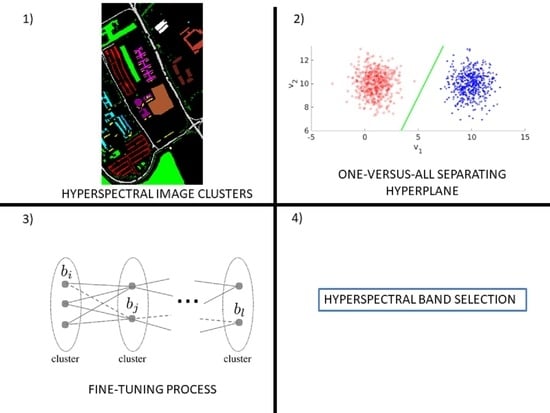
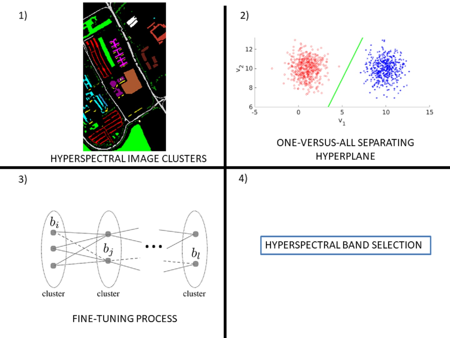
• The use of a cluster-wise approach to solving the unsupervised band selection problem;
• Once two clusters were formed, the selection of bands was based on the parameters of a hyperplane defined by a single-layer neural network;
• Fine-tuning of the selected bands based on cluster separability in the feature space.

In Section 2, the proposed method is presented. In Section 3, the results of the proposed method are compared to five competitors by using three classifiers and three hyperspectral images commonly used in BS literature. Finally, in Section 5, we offer the conclusion of this work.

2. Method

Every BS algorithm is supposed to select relevant features—refer to [39] for a thorough definition of feature relevance. In short, a relevant spectral band (i) should provide useful information [40]; and (ii) should not be redundant  [14]. Since the proposed band selection framework is designed for classification purposes, the bands considered to provide useful information are those that provide maximum separation between clusters in the feature space. When it comes to redundancy between spectral bands, in this work, it is measured by correlation.

Therefore, following this reasoning, the proposed method is composed of three parts: Data clustering; Selection of bands of interest; and Redundancy reduction.

2.1. Data Clustering

Regarding unsupervised problems—data reconstruction [2] and data structure analysis (DSA), for instance, are approaches that render feature selection feasible.

Data entry clustering can find natural groupings in data sets, and, for this reason, it is considered a DSA-based band selection approach, when used for this purpose.

Inspired by [41], the proposed method also performs clustering of the data entries. However, here, we adopted a partitional clustering instead of a hierarchical one, as illustrated in Figure 1a. With partitional clustering, each resulting cluster ${\mathbf{C}}_i$, $i\in \{1,2,\dots ,k\}$, could be taken as a representative of the real class if (i) k equals the number of classes present in the data set, and (ii), the clustering algorithm, is appropriate for the data set at hand.

One generally wants to classify objects present in a known scene, supposing one knows beforehand the number k of classes is plausible.

Choice of the Clustering Algorithm

As for the fitness of a clustering algorithm to hyperspectral data, 11 methods were evaluated. It is worth noting that our focus was not on the best clustering algorithm available in the literature, but rather just to use some well-established clustering algorithms to show the efficiency of the proposed method.

The input data are the Salinas hyperspectral image [42], with 224 bands and 16 classes.

So, each clustering algorithm was set to find $k=16$ clusters—as we will see later in this paper, the proposed method sets k equal to the number of classes in the image. It is important to clarify that, at this point, the focus is on the comparison of clustering methods, so the data labels will be used.

The measure of agreement between the two data sets—the clustering result and Salinas ground truth—was computed by means of the adjusted Rand index (r) [1]. In short, let ${\kappa }_1$ and ${\kappa }_2$ be two different clustering types of a given data set; where ${\kappa }_1$ is the real class of the Salinas image and ${\kappa }_2$ is the result of a clustering algorithm.

Considering all pairs of vectors ${\mathbf{x}}_j$ and ${\mathbf{x}}_l$, with $j\ne l$, let ${\alpha }_1$ be the number of times that both vectors belong to the same clusters in the clustering types ${\kappa }_1$ and ${\kappa }_2$. Moreover, let ${\alpha }_2$ be the number of times the vectors belong to different clusters in ${\kappa }_1$ and different clusters in ${\kappa }_2$.

Finally, the adjusted Rand index between clusters ${\kappa }_1$ and ${\kappa }_2$ is given by

$$r=({\alpha }_1+{\alpha }_2)/m,$$

(1)

where m is the number of possible vector pairs in the data set.

For each clustering algorithm, r was calculated 10 times.

Table 1. Adjusted Rand index ($0\le r\le 1$) (mean values out of 10 runs for Salinas HSI).

Clustering Algorithm	r
K-means (Euclidean)	0.6997
K-means (cityblock)	0.7382
K-means (cosine)	0.7941
K-means (correlation)	0.7170
K-medoids (Euclidean)	0.7062
K-medoids (Mahalanobis)	0.7685
K-medoids (cityblock)	0.7402
K-medoids (Minkowski)	0.7396
K-medoids (Chebychev)	0.7269
K-medoids (Spearman)	0.7674
K-medoids (Jaccard)	0.6146

shows the mean values for k-means and k-medoids algorithms with different distance metrics. K-means using the cosine similarity measure has the best outcome. For the sake of clarity, the bigger the values of r, the more similar the clustering types of ${\kappa }_1$ and ${\kappa }_2$.

Consequently, all of the clusters throughout this paper were obtained by k-means using the cosine similarity measure.

It is worth mentioning that an appropriate partitional clustering is able to turn supervised band selection algorithms into unsupervised ones, by taking the resulting clusters as class representatives, and the degree of success depends on r values. This paper follows that approach, by considering [4] as a reference. Since $0\le r\le 1$, where 1 means the two clustering outcomes match identically, $r=0.7941$ indicates a good match between the clusters and the real classes of Salinas HSI. At this point, we opted to analyze a hyperspectral image not used in Section 3 in order to maintain the unsupervised nature of the proposed approach.

2.2. Selection of Bands of Interest

Once the initial data set is split into k clusters, it is time to present the proposed band selection algorithm, which has k iterations. At each iteration, two steps take place: (i) the selection of candidate bands and (ii) fine-tuning.

2.2.1. Selection of Candidate Bands

Let ${\mathbf{C}}_0=[{\mathbf{b}}_1,{\mathbf{b}}_2,\dots ,{\mathbf{b}}_d]\in {\mathbb{R}}^{n\times d}$ be the initial cluster, i.e., the HSI, where $b_j$ is the $j^{th}$ band vector whose norm $l_2$ is scaled to 1, n is the number of pixels and d is the dimensionality of the data set.

Let ${\mathbf{C}}_i$, $\forall i\in \{1,2,\dots ,k\}$, be the k clusters after the partitional clustering of ${\mathbf{C}}_0$, where k is the number of classes in the data set.

The following properties hold for the clusters:

• ${\mathbf{C}}_i\ne \varnothing$, for $i\in \{1,2,\dots ,k\}$;
• ${\cup }_{i=1}^k{\mathbf{C}}_i={\mathbf{C}}_0$;
• ${\mathbf{C}}_i\cap {\mathbf{C}}_l=\varnothing$, with $i\ne l$ and $i,l\in \{1,2,\dots ,k\}$.

For each cluster, a one-versus-all binary classification was performed between ${\mathbf{C}}_i$ and ${\mathbf{C}}_0\setminus {\mathbf{C}}_i$.

As in [4], we used a single-layer neural network to generate the separating hyperplane f. As an illustration, both the one-versus-all classification and the hyperplane f are shown in Figure 1b.

The cross-entropy loss function of the neural network is given by

$$L_f=-\frac{1}{\eta }\sum _{j=1}^{\eta }[y_{j}log\left({\widehat{y}}_j\right)+(1-y_j)log(1-{\widehat{y}}_j)],$$

(2)

where $\eta$ is the cardinality of the set containing the data points —since we make $|{\mathbf{C}}_0\setminus {\mathbf{C}}_i|\approx |{\mathbf{C}}_i|$ in order to balance the two clusters, $\eta \le n$—; $y_j\in \{0,1\}$ is the expected output to the input vector ${\mathbf{x}}_j\in {\mathbb{R}}^{d\times 1}$, where label 1 corresponds to cluster ${\mathbf{C}}_i$; and ${\widehat{y}}_j$ is the calculated output given by

$${\widehat{y}}_j=\frac{1}{1+e^{z_j}},$$

(3)

which is the sigmoid activation function. where e is the Euler’s number, and $z_j$ is the hyperplane equation

$$z_j=x_j^{\left(1\right)}{w}^{\left(1\right)}+x_j^{\left(2\right)}{w}^{\left(2\right)}+\dots +x_j^{\left(d\right)}{w}^{\left(d\right)}+\beta ,$$

(4)

where $\mathbf{w}\in {\mathbb{R}}^{d\times 1}$ and $\beta \in \mathbb{R}$—both calculated by a single-layer neural network—are the hyperplane f parameters.

The training phase of the network consists of 2000 training epochs, using the backpropagation algorithm, with 70% of the data set for training and the remaining 30% for the test.

After the neural network’s training, a given input vector ${\mathbf{x}}_j$ will cause either $z_j\ge 0$ or $z_j<0$. As $z_j$ is the argument of a sigmoid function, if

• $z_j\ge 0$, then ${\widehat{y}}_j\leftarrow round\left({\widehat{y}}_j\right)=1$,
• $z_j<0$, then ${\widehat{y}}_j\leftarrow round\left({\widehat{y}}_j\right)=0$,

where $round({\widehat{y}}_j\ge 0.5)=1$, and $round({\widehat{y}}_j<0.5)=0$.

The band selection is based on the magnitude of weight vector components $w^{\left(l\right)}$, $l\in \{1,\dots ,d\}$. Indeed, according to (4), the biggest weights in magnitude, $|w^{\left(l\right)}|$, will strongly determine the signal of $z_j$. Therefore, the bands $x_j^{\left(l\right)}$—related to the biggest $|w^{\left(l\right)}|$—are the most relevant for the binary one-versus-all classification, and are, consequently, initially selected.

In order to provide an illustrative view on this matter, Figure 2 depicts a 2D situation in which a linear classifier, represented by a line segment, separates two different clusters, in red and blue colors, composed of synthetic data of variables $v_1$ and $v_2$. In Figure 2a, the clusters are linearly separable, and it is easy to perceive that this separation is provided by variable $v_2$, whereas variable $v_1$ bears similar values for both clusters. It is worth noting that the green line’s parameters $w^{\left(1\right)}$ and $w^{\left(2\right)}$, calculated by a single-layer neural network ($\beta$ is omitted), indicate the relative importance of variables in this binary classification. That is, $|w^{\left(2\right)}|=4.8126>|w^{\left(1\right)}|=0.5782$ indicates a higher relevance of variable $v_2$ in relation to $v_1$. A similar situation occurs in Figure 2b, but this time $|w^{\left(1\right)}|>|w^{\left(2\right)}|$, indicating that variable $v_1$ provides better separability between the clusters. Figure 2c,d shows that the same analysis is valid even when the clusters overlap.

According to the proposed method, the number s of selected bands is defined by the user.

Since the method has k iterations, the selection of $(s/k)\in \mathbb{N}$ bands per iteration would be sufficient. However, at each iteration, the method selects $4(s/k)$ bands, from which only $s/k$ are kept after the fine-tuning step. It is worth noting that, except for $4(s/k)$, other numbers have not been tested.

2.2.2. Fine-Tuning

At each iteration $i\in \{1,2,\dots ,k\}$, $4(s/k)$ bands are selected based on the biggest weights $|w^{\left(l\right)}|$, according to (4).

Those bands are then placed in $s/k$ clusters—by means of k-means (Euclidean)—$q_l$, $l\in \{1,2,\dots ,(s/k\left)\right\}$, and from each cluster 1 band $\mathbf{b}$ will be initially selected.

By picking 1 band from each cluster q, several tuples t are formed. An example of it is shown in Figure 3. The exact number of tuples is $|q_1|\times |q_2|\times \dots \times |q_{s/k}|$. Formally, at iteration i the set containing all tuples is given by

$$Q=\{({\mathbf{b}}_i^{\left(1\right)},\dots ,{\mathbf{b}}_j^{(s/k)}),{\mathbf{b}}_j^{\left(l\right)}\in q_l,l\in \{1,\dots ,(s/k)\}\}.$$

(5)

Note that this approach for refining the band selection is based on [43]; however, here we adopted a different criterion to assess the importance of each tuple of bands.

For each tuple $t\in Q$, its bands were evaluated according to the class separability they provided between ${\mathbf{C}}_i$ and ${\mathbf{C}}_0\setminus C_i$. At this point, the data sets of both clusters contain only the bands in t.

The class separability is measured by the $\rho \in \mathbb{R}$ index,

$$\rho =\frac{trace({\mathbf{S}}_w+{\mathbf{S}}_b)}{trace\left({\mathbf{S}}_w\right)},$$

(6)

where

$${\mathbf{S}}_w=p_{{\mathbf{C}}_i}{\Sigma }_{{\mathbf{C}}_i}+p_{(C_0\setminus {\mathbf{C}}_i)}{\Sigma }_{({\mathbf{C}}_0\setminus {\mathbf{C}}_i)},$$

and

$${\mathbf{S}}_b=p_{{\mathbf{C}}_i}({\mu }_{{\mathbf{C}}_i}-{\mu }_0)({\mu }_{({\mathbf{C}}_0\setminus {\mathbf{C}}_i)}-{\mu }_0)p_{({\mathbf{C}}_0\setminus {\mathbf{C}}_i)},$$

where ${\mu }_{{\mathbf{C}}_i}$ is the mean of cluster ${\mathbf{C}}_i$, ${\mu }_0$ is the global mean, $\Sigma$ is the covariance matrix, and p is the a priori probability. Since the clusters ${\mathbf{C}}_i$ and ${\mathbf{C}}_0\setminus {\mathbf{C}}_i$ are balanced, i.e., $|{\mathbf{C}}_i|=|{\mathbf{C}}_0\setminus {\mathbf{C}}_i|$, then $p_{{\mathbf{C}}_i}=p_{({\mathbf{C}}_0\setminus {\mathbf{C}}_i)}=0.5$.

According to (6), the bigger the $\rho$, the more compact the clusters are, and the more distant they are from each other.

Finally, for each tuple $t\in Q$ there is a corresponding $\rho$ value, and only the bands in $t^{max}$, whose $\rho$ is the biggest, are selected at iteration i.

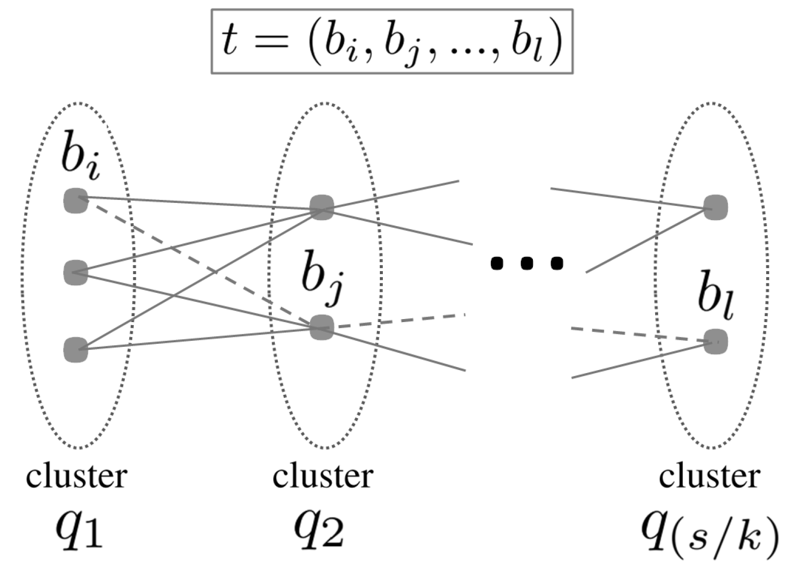
2.3. Redundancy Reduction

Let $\mathrm{\Psi }\in {\mathbb{R}}^{d\times d}$ be the correlation matrix of the data set ${\mathbf{C}}_0$, calculated according to Pearson’s correlation coefficient.

Let $\psi$ be a set composed of the bands the most correlated to the band represented by $\psi$ indices. Set $\psi$ is calculated before the iterations start, according to Algorithm 1. For the sake of clarity, ${\psi }_j={\mathbf{b}}_l$, for instance, means that ${\mathbf{b}}_l$ is the band the most correlated to band ${\mathbf{b}}_j$.

Algorithm 1 starts by creating a correlation matrix $\mathrm{\Psi }$, according to Pearson’s correlation. After the initialization of matrix $\mathbf{I}$ and vector $\psi$, we sort all the columns of $\mathrm{\Psi }$ in a descend fashion, and store the indices $idx$, which corresponds to the band indices. To the first position of $\psi$ is assigned the band ${\mathbf{b}}_{\mathbf{I}(1,1)}$. Then the remaining positions of $\psi$ receive the bands the most correlated to the band corresponding to that position in a way no same band is assigned to more than one position. The output is the vector $\psi$.

Given $t^{max}$ and $\psi$, the subset ${\delta }_{t^{max}}$ of the bands the most correlated to those in $t^{max}$ is given by Algorithm 2.

In Algorithm 2 we have $t^{max}$ and $\psi$ as input. Given the bands in $t^{max}$, the algorithm finds the most correlated bands to those in $t^{max}$ and insert them in subset ${\delta }_{t^{max}}$, which is the output of the algorithm.

Algorithm 1 Most correlated bands

1: $\mathrm{\Psi }=corr\left({\mathbf{C}}_0\right)$                ▷ Pearson’s correlation 2: Initialize matrix $\mathbf{I}$ 3: $\psi =\varnothing$ 4: for all the columns $\mathbf{c}\in \mathrm{\Psi }$ do 5:    $[values,idx]=sort(\mathbf{c},“descen{d}^{”})$        ▷$idx\in {\mathbb{N}}^{1\times d}$ 6:    $\mathbf{I}=[\mathbf{I};idx]$ 7: ${\psi }_1\leftarrow {\mathbf{b}}_{\mathbf{I}(1,1)}$ 8: for i = 2 : d do 9:    for j = 1 : d do 10:        if ${\mathbf{b}}_{\mathbf{I}(i,j)}\notin \psi$ then 11:           $\psi \leftarrow \psi \cup {\mathbf{b}}_{\mathbf{I}(i,j)}$ 12:           Break 13: Return: $\psi$

Algorithm 2 The most correlated bands to a given subset

1: Input: $t^{max}$, $\psi$ 2: ${\delta }_{t^{max}}=\varnothing$ 3: for j = 1 : $|t^{max}|$ do          ▷ Vector cardinality 4:    for l = 1 : $\left|\psi \right|$ do 5:        if ${\psi }_l=t_j^{max}$ then 6:           ${\delta }_{t^{max}}\leftarrow {\delta }_{t^{max}}\cup b_l$ 7: Return: ${\delta }_{t^{max}}$

Finally, at each iteration i, the bands in $t^{max}$ are selected and inserted in $\mathbf{S}$, which is the final subset of selected bands. So,

$$\mathbf{S}\leftarrow \mathbf{S}\cup t^{max}.$$

(7)

Once we have $t^{max}$, its most correlated bands ${\delta }_{t^{max}}$ are inserted in subset $\mathbf{D}$, which are the bands to be discarded. That is,

$$\mathbf{D}\leftarrow \mathbf{D}\cup {\delta }_{t^{max}}.$$

(8)

Then, for the next iteration $i+1$ the data set is updated according to

$${\mathbf{C}}_0\leftarrow {\mathbf{C}}_0\setminus (\mathbf{S}\cup \mathbf{D}).$$

(9)

The method iterates until $i=k$. Then, the final output is the subset $\mathbf{S}$ of selected bands.

2.4. Proposed Method’s Overview

Algorithm 3 presents the overview of the proposed method.

Algorithm 3 Proposed band selection algorithm

1: Input: Data set ${\mathbf{C}}_0$, number k of classes 2: $\mathbf{S}=\varnothing$                       ▷ Subset of selected bands 3: $\mathbf{D}=\varnothing$                    ▷ Subset of bands to be discarded 4: Proceed to k-means clustering (cosine distance) of ${\mathbf{C}}_0$ into k clusters ${\mathbf{C}}_i$ 5: for i = 1 : k do 6:    Proceed to a binary classification between clusters ${\mathbf{C}}_i$ and ${\mathbf{C}}_0\setminus {\mathbf{C}}_i$ (one-versus-all)  using a single-layer neural net 7:    Select the $4(s/k)\in \mathbb{N}$ bands related to the biggest separating hyperplane parameters  $\left|w\right|$, according to (4) 8:    Proceed to the band selection fine-tuning, according to Section 2.2.2 9:    Update subset of selected bands $\mathbf{S}$ according to (7) 10:    Update subset $\mathbf{D}$ according to (8) 11:    Update data set according to (9) 12: Return: S

3. Results

Normally the quality of the subset of selected bands is assessed by the performance of the classifiers. So, this approach is adopted here, with support vector machine (SVM), K-nearest neighbor (KNN), and classification and regression tree (CART) classifiers [1], via three hyperspectral data sets used in several BS papers: Botswana, Indian Pines, and Pavia University. All of them can be downloaded at [42].

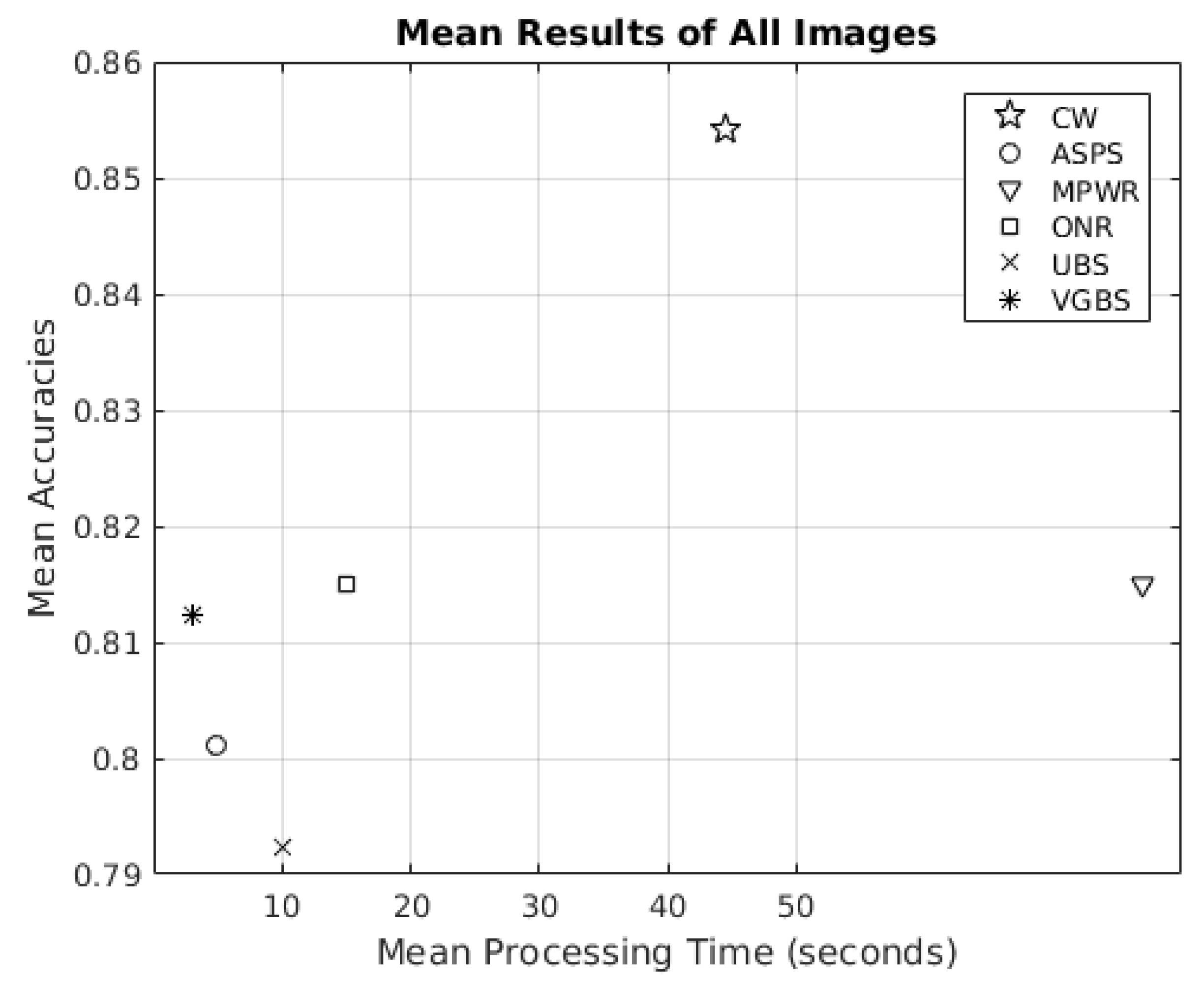
3.1. Competitors

The proposed method is compared to five state-of-the-art BS methods: ASPS, MPWR, ONR, UBS, and VGBS.

3.1.1. ASPS

ASPS [44] is the acronym for hyperspectral band selection via adaptive subspace partition strategy. Its framework begins with a two-step partition of the data cube, starting with the coarse partition of the image cube into a predetermined number of parts, and then there is a fine subspace partition, from which bands with low noise levels are finally selected.

3.1.2. MPWR

In [45], the authors proposed a manifold-preserving and weakly redundant (MPWR) unsupervised band selection method. A manifold-preserving band-importance metric was used to measure the band-wise essentiality. Concerning the redundancy caused by the correlated bands, this paper establishes a constrained band-weight optimization model. Thus, both band-wise manifold-preserving capability and intraband correlation are integrated into the BS method.

3.1.3. ONR

The approach called ’hyperspectral band selection via optimal neighborhood reconstruction’ is based on optimal neighborhood reconstruction (ONR) [46]. It proceeds to different band combinations in order to reconstruct the original data set, and also applies a noise reducer to minimize the influence of noisy bands.

3.1.4. UBS

UBS is used as the acronym for the approach presented in [47]. This method is based on the spectral decomposition of a matrix, then the loading-factors matrix can be constructed for band prioritization, according to the corresponding eigenvalues and eigenvectors.

3.1.5. VGBS

This paper states that there is a relation between the volume of a sub-simplex and the volume gradient of a simplex. Based on this, they proposed a BS method called VGBS [48]. It is unsupervised and seeks to remove the most redundant band based only on the gradient of volume instead of calculating the volumes of all sub-simplexes.

3.2. Experimental Results

In order to compare the outcome of the proposed method, five different bands were selected from scratch: 10, 20, 30, 40, and 50. A set with 50 bands does not necessarily contain the 10-band set, for example, due to the nature of the neural networks.

We compare the results to other BS methods for each hyperspectral image separately. All of the classifier accuracies exhibited here are the mean values of ten runs.

Our approach is dubbed CW—the unsupervised cluster-wise method.

3.2.1. (Case 1) Botswana HSI

The Botswana image is composed of 242 spectral bands and has 14 classes. See further details about this image at [42].

Table 2. Botswana image results (overall accuracy and standard deviation in %).

Method	10 Bands	20 Bands	30 Bands	40 Bands	50 Bands
			KNN classifier
CW	90.86 ± 0.69	88.81 ± 0.27	90.86 ± 0.91	91.48 ± 0.97	93.22 ± 0.69
ASPS	85.63 ± 0.75	89.73 ± 0.94	91.07 ± 0.76	89.01 ± 0.63	91.58 ± 0.72
MPWR	81.52 ± 0.99	86.45 ± 1.43	90.76 ± 0.56	90.35 ± 1.05	90.25 ± 0.89
ONR	90.66 ± 0.91	$\mathbf{92}.\mathbf{61}$ ± 0.53	89.94 ± 0.64	91.38 ± 0.89	91.99 ± 0.86
UBS	88.50 ± 1.07	89.53 ± 1.05	87.99 ± 0.86	89.94 ± 0.66	90.04 ± 0.96
VGBS	88.09 ± 0.79	90.55 ± 1.00	88.50 ± 1.30	87.17 ± 1.29	88.09 ± 1.10
			CART classifier
CW	84.80 ± 1.23	86.55 ± 1.27	84.91 ± 1.49	85.93 ± 1.03	86.04 ± 1.13
ASPS	81.72 ± 1.04	85.32 ± 1.27	83.78 ± 1.15	83.98 ± 1.38	84.50 ± 0.96
MPWR	72.59 ± 1.27	81.31 ± 1.13	84.29 ± 1.02	85.52 ± 1.13	85.01 ± 1.47
ONR	83.37 ± 0.74	84.80 ± 1.35	84.91 ± 1.06	84.60 ± 1.01	84.70 ± 1.46
UBS	80.39 ± 1.14	83.26 ± 1.07	83.68 ± 1.36	85.32 ± 0.84	85.01 ± 0.98
VGBS	83.98 ± 0.81	85.22 ± 0.95	82.24 ± 1.35	83.47 ± 0.65	86.24 ± 1.44
			SVM classifier
CW	89.73 ± 0.72	94.76 ± 0.91	94.97 ± 0.69	93.94 ± 0.61	94.15 ± 0.56
ASPS	87.78 ± 0.67	91.27 ± 0.67	93.84 ± 0.66	92.09 ± 0.69	94.05 ± 0.55
MPWR	87.06 ± 1.06	90.86 ± 0.97	93.73 ± 0.67	94.76 ± 0.75	94.15 ± 0.61
ONR	92.91 ± 0.36	94.25 ± 0.48	93.83 ± 0.62	94.76 ± 0.46	94.14 ± 0.77
UBS	89.42 ± 0.82	92.50 ± 0.98	92.71 ± 0.67	93.42 ± 0.86	92.91 ± 0.89
VGBS	90.04 ± 0.97	92.81 ± 0.58	93.63 ± 1.06	93.01 ± 0.68	93.53 ± 0.65

shows the results of the BS methods using Botswana HSI. Bold values represent the highest scores attained. Figure 4 presents the same results in an illustrative way. In the figure, different marks are used in order to identify the competitors. The line connecting the marks does not mean interpolation, but rather helps the reader.

Since the Botswana image has 14 classes, the proposed method has the same number of iterations—see Algorithm 3. For each one-versus-all case, a single-layer neural net is run, and the error (of the test set) versus the epoch curves are shown in Figure 5. Clearly, there is convergence in all cases, meaning that it is possible to find a hyperplane to separate the clusters ${\mathbf{C}}_i$ and ${\mathbf{C}}_0\setminus {\mathbf{C}}_i$. The different curve shapes indicate how fast the algorithm converged. For instance, in Figure 5, Cluster 1 versus All converged faster than Cluster 6 versus All.

Concerning the results, there were five different sets of selected bands, and each set was subjected to three classifiers. Thus, in total, we had 15 different experiments, from which the proposed CW framework surpassed its competitors in 9 out of 15 cases.

3.2.2. (Case 2) Indian Pines HSI

This image has 224 bands and 16 classes. Further details about this image can be found at [42].

Table 3. Indian Pines image results (overall accuracy and standard deviation in %).

Method	10 Bands	20 Bands	30 Bands	40 Bands	50 Bands
			KNN classifier
CW	76.81 ± 1.13	80.00 ± 0.54	78.14 ± 0.31	81.13 ± 0.59	79.45 ± 0.70
ASPS	68.61 ± 0.68	66.50 ± 0.93	66.41 ± 0.90	63.19 ± 0.33	63.32 ± 0.27
MPWR	69.66 ± 0.89	70.63 ± 0.59	72.52 ± 0.43	73.59 ± 0.49	70.63 ± 1.12
ONR	71.35 ± 0.35	70.99 ± 0.61	67.41 ± 1.62	71.45 ± 0.57	72.03 ± 0.96
UBS	64.62 ± 0.52	63.15 ± 0.69	64.78 ± 1.09	64.98 ± 0.82	63.22 ± 0.72
VGBS	69.14 ± 0.80	70.21 ± 0.90	67.94 ± 0.74	70.41 ± 0.55	69.98 ± 0.61
			CART classifier
CW	70.82 ± 0.78	74.21 ± 0.67	72.55 ± 0.86	73.50 ± 0.70	72.75 ± 0.81
ASPS	69.49 ± 0.41	69.20 ± 0.33	71.94 ± 0.46	73.20 ± 0.77	73.20 ± 0.58
MPWR	63.45 ± 0.66	67.32 ± 0.73	70.73 ± 0.70	71.58 ± 0.65	71.28 ± 0.88
ONR	71.28 ± 0.99	75.41 ± 0.76	73.30 ± 1.40	74.57 ± 1.22	73.33 ± 0.82
UBS	71.71 ± 0.96	73.66 ± 0.78	74.67 ± 0.83	74.24 ± 1.12	73.69 ± 0.86
VGBS	70.44 ± 0.30	70.60 ± 0.57	71.22 ± 1.28	70.83 ± 0.75	71.32 ± 0.78
			SVM classifier
CW	84.58 ± 0.80	86.70 ± 0.16	84.29 ± 5.14	87.97 ± 4.48	87.61 ± 0.78
ASPS	81.39 ± 0.58	80.36 ± 0.65	82.60 ± 0.58	80.72 ± 0.52	83.68 ± 0.20
MPWR	72.88 ± 0.95	78.82 ± 0.64	81.07 ± 0.82	84.39 ± 0.50	83.77 ± 0.50
ONR	82.70 ± 0.31	84.75 ± 0.70	84.10 ± 0.60	86.93 ± 0.82	84.88 ± 4.00
UBS	79.61 ± 0.51	82.86 ± 0.23	76.91 ± 0.61	82.08 ± 0.37	79.94 ± 3.60
VGBS	76.59 ± 0.70	79.97 ± 0.79	79.06 ± 0.52	80.68 ± 0.75	80.07 ± 1.04

shows the accuracies and standard deviations of the results.

Out of 15 experiments, the proposed CW method achieved the best results 10 times. In Figure 6, it is possible to have a visual idea of the performance of all BS methods.

According to Figure 7, for all iterations, the single-layer neural network converged. This convergence is seen by the fact that the error was lower as the number of epochs increased.

3.2.3. (Case 3) Pavia University HSI

This image has 102 spectral bands and 9 classes. See more information about this image at [42].

In

Table 4. Pavia University image results (overall accuracy and standard deviation in %).

Method	10 Bands	20 Bands	30 Bands	40 Bands	50 Bands
			KNN classifier
CW	92.19 ± 0.26	92.12 ± 0.48	91.73 ± 0.15	90.37 ± 0.24	90.99 ± 0.15
ASPS	87.67 ± 0.11	90.24 ± 0.39	89.90 ± 0.39	89.33 ± 0.29	90.54 ± 0.40
MPWR	91.80 ± 0.39	90.99 ± 0.14	92.37 ± 0.93	90.45 ± 0.41	91.19 ± 1.19
ONR	88.89 ± 0.19	92.30 ± 0.15	91.82 ± 0.29	91.02 ± 0.16	91.60 ± 0.11
UBS	86.00 ± 0.42	88.15 ± 0.44	87.84 ± 0.22	88.10 ± 0.22	88.17 ± 0.10
VGBS	84.26 ± 0.39	87.77 ± 0.34	86.42 ± 0.28	87.24 ± 0.39	88.30 ± 0.60
			CART classifier
CW	89.54 ± 0.12	89.18 ± 0.35	89.31 ± 0.29	89.04 ± 0.39	89.04 ± 0.37
ASPS	83.23 ± 0.35	86.69 ± 0.26	86.74 ± 0.48	87.06 ± 0.37	86.47 ± 0.10
MPWR	89.29 ± 0.67	88.82 ± 0.83	89.67 ± 0.71	89.03 ± 0.95	88.81 ± 0.81
ONR	85.37 ± 0.13	89.63 ± 0.23	89.03 ± 0.26	88.69 ± 0.16	89.00 ± 0.25
UBS	85.02 ± 0.49	87.27 ± 0.43	86.26 ± 0.31	86.50 ± 0.23	87.42 ± 0.36
VGBS	85.79 ± 0.23	88.26 ± 0.31	88.12 ± 0.32	88.49 ± 0.20	88.04 ± 0.31
			SVM classifier
CW	94.97 ± 2.38	90.77 ± 12.59	75.56 ± 16.17	68.26 ± 16.51	67.01 ± 15.36
ASPS	89.58 ± 9.48	88.67 ± 9.41	40.19 ± 12.39	48.71 ± 15.96	40.56 ± 10.81
MPWR	94.93 ± 3.95	91.85 ± 8.64	70.66 ± 13.81	39.13 ± 17.51	54.86 ± 15.50
ONR	91.31 ± 12.39	52.29 ± 24.56	46.62 ± 10.86	43.36 ± 21.41	43.48 ± 12.96
UBS	89.32 ± 2.49	54.75 ± 18.87	53.18 ± 13.99	38.06 ± 16.05	45.21 ± 13.29
VGBS	91.29 ± 13.59	89.74 ± 14.54	74.77 ± 17.88	50.58 ± 8.86	51.20 ± 12.23

, we see the results, in terms of overall accuracy and standard deviation, of all methods. The proposed CW algorithm has the best accuracies in 8 out of 15 experiments. It is also shown in Figure 8.

Figure 9 indicates that all the one-versus-all separating hyperplanes solutions converged.

3.3. Remark

Finally, since this is a paper about band selection,

Table 5. All the bands selected by the proposed CW method.

Number of Bands	Selected Bands
	Botswana image
10	4 11 17 21 24 41 69 101 105 120
20	7 10 12 28 32 33 37 39 40 49 55 58 59 65 67 73 75 76 113 124
30	2 4 5 7 21 27 29 30 32 33 34 35 37 43 44 47 54 56 57 58 61 62 71 74 78 80 82 118 120 124
40	2 3 4 5 6 8 13 14 16 27 28 31 32 33 34 35 36 39 41 42 52 54 58 60 63 65 69 70 72 74 78 88 89 92 97 100 101 105 135 142
50	1 2 4 5 6 8 10 16 19 21 22 23 24 25 26 27 30 31 32 33 34 36 41 42 47 57 58 59 66 67 69 72 74 75 77 78 87 89 94 96 98 100 101 102 104 109 110 113 130 144
	Indian Pines image
10	16 20 21 33 34 39 92 97 119 128
20	8 10 15 16 17 19 26 27 30 33 36 43 46 47 64 78 97 98 117 133
30	5 6 7 8 9 15 27 30 35 37 39 40 46 56 57 62 63 64 71 73 74 75 76 78 82 92 98 168 173 174
40	4 6 7 9 10 16 17 19 27 30 32 33 34 35 36 40 46 50 52 53 57 63 69 72 74 84 92 93 97 99 100 117 121 122 126 137 139 140 142 199
50	6 9 11 12 15 20 22 23 25 26 29 30 31 32 33 36 41 42 43 44 45 46 49 50 51 55 56 59 65 71 73 74 75 76 77 84 92 95 98 102 114 117 119 121 122 130 138 168 172 199
	Pavia University image
10	21 42 55 70 72 73 75 83 85 98
20	15 18 28 46 49 55 56 60 61 63 65 71 83 85 88 89 91 95 99 103
30	10 16 20 22 31 36 38 40 50 54 59 61 62 64 65 67 70 72 74 77 80 83 85 91 92 94 96 98 100 102
40	3 10 11 14 16 17 18 20 23 27 38 39 44 46 51 56 58 59 61 62 63 65 67 69 71 72 74 75 76 78 80 83 84 85 91 94 96 98 100 103
50	9 10 11 13 15 17 18 20 23 25 26 28 29 31 33 35 37 40 41 44 56 57 59 61 62 63 65 66 67 69 71 72 73 75 77 79 81 83 84 85 88 90 92 94 95 96 98 100 102 103

presents all of the bands selected by the proposed method CW.

4. Discussion

The proposed method was introduced in Section 2.2 and its performance was reviewed in Section 3.2.

It is still important to emphasize the advantages of using the proposed method CW. On the other hand, the deficiencies of the algorithm will also be highlighted.

4.1. Pros

As shown in Table 2, Table 3 and Table 4, with their corresponding Figure 4, Figure 6 and Figure 8, each classifier, due to its intrinsic characteristics, performed differently when compared to the others. SVM classifiers are well known for their effectiveness in high-dimensional spaces, such as the feature space of a hyperspectral image. Thus, for this reason, we see SVM outperforming the other classifiers. On this topic, we see an exception in Table 4 and Figure 8, where SVM is less accurate than the other two classifiers. Given that KNN and CART exhibit stable performances as the band numbers increase, the reason for the bad performance of SVM, in this case, as the dimensionality became higher, may lie in the fact that the Pavia University data were not well discriminative for the SVM algorithm (this phenomenon happened with all competitors). When it comes to the KNN classifier, we set the number of neighbors equal to 7, i.e., $K=7$ in all experiments; the objective here was not to find the best settings for the KNN but to provide equal conditions for the comparison of the band selection methods. As KNN classifies an input pattern based on its neighbors in the feature space, it performed better than the CART classifier, whose decision trees rely on binary rules, which become more complex as dimensionality increases.

In general, the proposed CW method outperformed its competitors in lower dimensions, due to the fact that the CW algorithm selected its bands based on the class separations in the feature space. Thus, even in lower dimensions, we saw a good performance of the proposed method, which was designed to be used as a filter method, i.e., a preprocessing step of hyperspectral data classification tasks. As the dimension increased, the CW method maintained good results when compared to its competitors. In fact, considering all of the results, we see that the proposed method achieved the best results in $\frac{9+10+8}{45}=60\%$ in the experiments. This is likely due to the fact that the CW method is capable of selecting the best spectral bands for each individual cluster (or class) in a one-versus-all fashion, even in an unsupervised case. Moreover, the cluster separability criterion used during the band selection process makes the job of the classifiers easier.

In terms of processing times, the proposed method does not appear amongst the fastest ones, as Figure 10 indicates. However, its outstanding accuracy mean compensates for this fact. Moreover, the mean processing time of the CW method was less than 50 s, which caused no problems in offline applications.

4.2. Cons

The proposed CW algorithm is not capable of addressing all the issues concerning a band selection application, such as the optimal number of bands to be selected. In fact, we do not address this topic in this paper. Here, the number s of bands to be selected is a user-defined parameter.

Moreover, it is necessary to know the number k of classes in the scene depicted by the image. Even though a remote sensing expert may easily infer the number of classes in a given scene, this topic remains unsolved.

5. Conclusions

The high dimensionality of a hyperspectral image can be useful in terms of good discrimination amongst objects and classes. On the other hand, it can also be a source of problems, such as the curse of dimensionality and overfitting of the classifier.

In order to alleviate such issues, this paper proposes a novel unsupervised band selection framework based on partitional clustering, in which each cluster stands for a real class of the data set. A hyperplane was used to separate all clusters in a one-versus-all fashion. After this, we proceeded to fine-tuning the initially selected bands based on the cluster separability in the feature space.

The proposed method achieved the best classification results in 60% of the experiments.

In future works, it is advisable to verify the performance of support vector machines to find a separating hyperplane between clusters. Furthermore, other numbers of initially chosen bands should be tested, rather than only $4(s/k)$. Moreover, some more recent clustering algorithms could be tested in order to check their effects on the final results. Finally, one could use optimization algorithms to find a suitable subset of bands during the fine-tuning process.

References

- Theodoridis, S.; Koutroumbas, K. Pattern Recognition, 4th ed.; Elsevier: Amsterdam, The Netherlands, 2009. [Google Scholar]
- Guyon, I.; Elisseeff, A. An Introduction to Variable and Feature Selection. J. Mach. Learn. Res. 2003, 3, 1157–1182. [Google Scholar]
- Chen, C.H. Statistical Pattern Recognition, 1st ed.; Spartan Books: Washington, DC, USA, 1973. [Google Scholar]
- Habermann, M.; Frémont, V.; Shiguemori, E.H. Supervised band selection in hyperspectral images using single-layer neural networks. Int. J. Remote Sens. 2019, 40, 3900–3926. [Google Scholar] [CrossRef]
- Houle, M.E.; Kriegel, H.P.; Kröger, P.; Schubert, E.; Zimek, A. Can Shared-Neighbor Distances Defeat the Curse of Dimensionality? In Scientific and Statistical Database Management; Gertz, M., Ludäscher, B., Eds.; Springer: Berlin/Heidelberg, Germany, 2010; pp. 482–500. [Google Scholar]
- Duda, R.O.; Hart, P.E.; Stork, D.G. Pattern Classification, 2nd ed.; Wiley: New York, NY, USA, 2001. [Google Scholar]
- Haykin, S.S. Neural Networks and Learning Machines, 3rd ed.; Pearson Education: Upper Saddle River, NJ, USA, 2009. [Google Scholar]
- Kuncheva, L.I.; Matthews, C.E.; Arnaiz-González, Á.; Rodríguez, J.J. Feature Selection from High-Dimensional Data with Very Low Sample Size: A Cautionary Tale. arXiv 2020, arXiv:abs/2008.12025. [Google Scholar]
- Shang, X.; Song, M.; Wang, Y.; Yu, C.; Yu, H.; Li, F.; Chang, C. Target-Constrained Interference-Minimized Band Selection for Hyperspectral Target Detection. IEEE Trans. Geosci. Remote Sens. 2020, 59, 6044–6064. [Google Scholar] [CrossRef]
- Zeng, M.; Cai, Y.; Cai, Z.; Liu, X.; Hu, P.; Ku, J. Unsupervised Hyperspectral Image Band Selection Based on Deep Subspace Clustering. IEEE Geosci. Remote Sens. Lett. 2019, 16, 1889–1893. [Google Scholar] [CrossRef]
- Feng, J.; Chen, J.; Sun, Q.; Shang, R.; Cao, X.; Zhang, X.; Jiao, L. Convolutional Neural Network Based on Bandwise-Independent Convolution and Hard Thresholding for Hyperspectral Band Selection. IEEE Trans. Cybern. 2021, 51, 4414–4428. [Google Scholar] [CrossRef] [PubMed]
- Ding, X.; Li, H.; Yang, J.; Dale, P.; Chen, X.; Jiang, C.; Zhang, S. An Improved Ant Colony Algorithm for Optimized Band Selection of Hyperspectral Remotely Sensed Imagery. IEEE Access 2020, 8, 25789–25799. [Google Scholar] [CrossRef]
- Bevilacqua, M.; Berthoumieu, Y. Multiple-Feature Kernel-Based Probabilistic Clustering for Unsupervised Band Selection. IEEE Trans. Geosci. Remote Sens. 2019, 57, 6675–6689. [Google Scholar] [CrossRef]
- Tang, J.; Alelyani, S.; Liu, H. Feature selection for classification: A review. In Data Classification; CRC Press: Boca Raton, FL, USA, 2014; pp. 37–64. [Google Scholar] [CrossRef]
- Liu, T.; Xiao, J.; Huang, Z.; Kong, E.; Liang, Y. BP Neural Network Feature Selection Based on Group Lasso Regularization. In Proceedings of the 2019 Chinese Automation Congress (CAC), Hangzhou, China, 22–24 November 2019; pp. 2786–2790. [Google Scholar] [CrossRef]
- Cao, X.; Xiong, T.; Jiao, L. Supervised Band Selection Using Local Spatial Information for Hyperspectral Image. IEEE Geosci. Remote Sens. Lett. 2016, 13, 329–333. [Google Scholar] [CrossRef]
- Gao, J.; Du, Q.; Gao, L.; Sun, X.; Wu, Y.; Zhang, B. Ant colony optimization for supervised and unsupervised hyperspectral band selection. In Proceedings of the 2013 5th Workshop on Hyperspectral Image and Signal Processing: Evolution in Remote Sensing (WHISPERS), Gainesville, FL, USA, 25–28 June 2013; pp. 1–4. [Google Scholar] [CrossRef]
- Habermann, M.; Frémont, V.; Shiguemori, E.H. Problem-based band selection for hyperspectral images. In Proceedings of the 2017 IEEE International Geoscience and Remote Sensing Symposium (IGARSS), Fort Worth, TX, USA, 23–28 July 2017; pp. 1800–1803. [Google Scholar] [CrossRef]
- Wei, X.; Cai, L.; Liao, B.; Lu, T. Local-View-Assisted Discriminative Band Selection with Hypergraph Autolearning for Hyperspectral Image Classification. IEEE Trans. Geosci. Remote Sens. 2020, 58, 2042–2055. [Google Scholar] [CrossRef]
- Feng, J.; Jiao, L.; Liu, F.; Sun, T.; Zhang, X. Mutual-Information-Based Semi-Supervised Hyperspectral Band Selection with High Discrimination, High Information, and Low Redundancy. IEEE Trans. Geosci. Remote Sens. 2015, 53, 2956–2969. [Google Scholar] [CrossRef]
- Guo, Z.; Yang, H.; Bai, X.; Zhang, Z.; Zhou, J. Semi-supervised hyperspectral band selection via sparse linear regression and hypergraph models. In Proceedings of the 2013 IEEE International Geoscience and Remote Sensing Symposium—IGARSS, Melbourne, Australia, 21–26 July 2013; pp. 1474–1477. [Google Scholar] [CrossRef]
- Cao, X.; Wei, C.; Ge, Y.; Feng, J.; Zhao, J.; Jiao, L. Semi-Supervised Hyperspectral Band Selection Based on Dynamic Classifier Selection. IEEE J. Sel. Top. Appl. Earth Obs. Remote Sens. 2019, 12, 1289–1298. [Google Scholar] [CrossRef]
- Bai, J.; Xiang, S.; Shi, L.; Pan, C. Semisupervised Pair-Wise Band Selection for Hyperspectral Images. IEEE J. Sel. Top. Appl. Earth Obs. Remote Sens. 2015, 8, 2798–2813. [Google Scholar] [CrossRef]
- Karoui, M.S.; Djerriri, K.; Boukerch, I. Unsupervised Hyperspectral Band Selection by Sequentially Clustering A Mahalanobis-Based Dissimilarity of Spectrally Variable Endmembers. In Proceedings of the 2020 Mediterranean and Middle-East Geoscience and Remote Sensing Symposium (M2GARSS), Tunis, Tunisia, 9–11 March 2020; pp. 33–36. [Google Scholar] [CrossRef]
- Sui, C.; Tian, Y.; Xu, Y.; Xie, Y. Unsupervised Band Selection by Integrating the Overall Accuracy and Redundancy. IEEE Geosci. Remote Sens. Lett. 2015, 12, 185–189. [Google Scholar] [CrossRef]
- Yang, C.; Bruzzone, L.; Zhao, H.; Tan, Y.; Guan, R. Superpixel-Based Unsupervised Band Selection for Classification of Hyperspectral Images. IEEE Trans. Geosci. Remote Sens. 2018, 56, 7230–7245. [Google Scholar] [CrossRef]
- Wang, Q.; Zhang, F.; Li, X. Optimal Clustering Framework for Hyperspectral Band Selection. IEEE Trans. Geosci. Remote Sens. 2018, 56, 5910–5922. [Google Scholar] [CrossRef]
- Xu, B.; Li, X.; Hou, W.; Wang, Y.; Wei, Y. A Similarity-Based Ranking Method for Hyperspectral Band Selection. IEEE Trans. Geosci. Remote Sens. 2021, 59, 9585–9599. [Google Scholar] [CrossRef]
- Datta, A.; Ghosh, S.; Ghosh, A. Combination of Clustering and Ranking Techniques for Unsupervised Band Selection of Hyperspectral Images. IEEE J. Sel. Top. Appl. Earth Obs. Remote Sens. 2015, 8, 2814–2823. [Google Scholar] [CrossRef]
- Jia, S.; Tang, G.; Zhu, J.; Li, Q. A Novel Ranking-Based Clustering Approach for Hyperspectral Band Selection. IEEE Trans. Geosci. Remote Sens. 2016, 54, 88–102. [Google Scholar] [CrossRef]
- Xie, W.; Lei, J.; Yang, J.; Li, Y.; Du, Q.; Li, Z. Deep Latent Spectral Representation Learning-Based Hyperspectral Band Selection for Target Detection. IEEE Trans. Geosci. Remote Sens. 2020, 58, 2015–2026. [Google Scholar] [CrossRef]
- Zhang, F.; Wang, Q.; Li, X. Hyperspectral image band selection via global optimal clustering. In Proceedings of the 2017 IEEE International Geoscience and Remote Sensing Symposium (IGARSS), Fort Worth, TX, USA, 23–28 July 2017; pp. 1–4. [Google Scholar] [CrossRef]
- Tang, G.; Jia, S.; Li, J. An enhanced density peak-based clustering approach for hyperspectral band selection. In Proceedings of the 2015 IEEE International Geoscience and Remote Sensing Symposium (IGARSS), Milan, Italy, 26–31 July 2015; pp. 1116–1119. [Google Scholar] [CrossRef]
- Sun, W.; Peng, J.; Yang, G.; Du, Q. Correntropy-Based Sparse Spectral Clustering for Hyperspectral Band Selection. IEEE Geosci. Remote Sens. Lett. 2020, 17, 484–488. [Google Scholar] [CrossRef]
- Kumar, V.; Hahn, J.; Zoubir, A.M. Band selection for hyperspectral images based on self-tuning spectral clustering. In Proceedings of the 21st European Signal Processing Conference (EUSIPCO 2013), Marrakech, Morocco, 9–13 September 2013; pp. 1–5. [Google Scholar]
- Dou, Z.; Gao, K.; Zhang, X.; Wang, H.; Han, L. Band Selection of Hyperspectral Images Using Attention-Based Autoencoders. IEEE Geosci. Remote Sens. Lett. 2021, 18, 147–151. [Google Scholar] [CrossRef]
- Damodaran, B.B.; Courty, N.; Lefèvre, S. Sparse Hilbert Schmidt Independence Criterion and Surrogate-Kernel-Based Feature Selection for Hyperspectral Image Classification. IEEE Trans. Geosci. Remote Sens. 2017, 55, 2385–2398. [Google Scholar] [CrossRef]
- Sun, W.; Peng, J.; Yang, G.; Du, Q. Fast and Latent Low-Rank Subspace Clustering for Hyperspectral Band Selection. IEEE Trans. Geosci. Remote Sens. 2020, 58, 3906–3915. [Google Scholar] [CrossRef]
- Kohavi, R.; John, G.H. Wrappers for Feature Subset Selection. Artif. Intell. 1997, 97, 273–324. [Google Scholar] [CrossRef]
- Cai, Y.; Liu, X.; Cai, Z. BS-Nets: An End-to-End Framework for Band Selection of Hyperspectral Image. IEEE Trans. Geosci. Remote Sens. 2020, 58, 1969–1984. [Google Scholar] [CrossRef]
- Habermann, M.; Frémont, V.; Shiguemori, E.H. Unsupervised Hyperspectral Band Selection Using Clustering and Single-Layer Neural Network. Revue Française de Photogrammétrie et de Télédétection 2018, 217–218, 33–42. [Google Scholar] [CrossRef]
- Graña, M.; Veganzons, M.A.; Ayerdi, B. Hyperspectral Remote Sensing Scenes. Available online: http://www.ehu.eus/ccwintco/index.php/Hyperspectral_Remote_Sensing_Scenes (accessed on 16 August 2022).
- Fu, X.; Shang, X.; Sun, X.; Yu, H.; Song, M.; Chang, C.I. Underwater Hyperspectral Target Detection with Band Selection. Remote Sens. 2020, 12, 1056. [Google Scholar] [CrossRef]
- Wang, Q.; Li, Q.; Li, X. Hyperspectral Band Selection via Adaptive Subspace Partition Strategy. IEEE J. Sel. Top. Appl. Earth Obs. Remote Sens. 2019, 12, 4940–4950. [Google Scholar] [CrossRef]
- Sui, C.; Li, C.; Feng, J.; Mei, X. Unsupervised Manifold-Preserving and Weakly Redundant Band Selection Method for Hyperspectral Imagery. IEEE Trans. Geosci. Remote Sens. 2020, 58, 1156–1170. [Google Scholar] [CrossRef]
- Wang, Q.; Zhang, F.; Li, X. Hyperspectral Band Selection via Optimal Neighborhood Reconstruction. IEEE Trans. Geosci. Remote Sens. 2020, 58, 8465–8476. [Google Scholar] [CrossRef]
- Chang, C.-I.; Du, Q.; Sun, T.-L.; Althouse, M.L.G. A joint band prioritization and band-decorrelation approach to band selection for hyperspectral image classification. IEEE Trans. Geosci. Remote Sens. 1999, 37, 2631–2641. [Google Scholar] [CrossRef]
- Geng, X.; Sun, K.; Ji, L.; Zhao, Y. A Fast Volume-Gradient-Based Band Selection Method for Hyperspectral Image. IEEE Trans. Geosci. Remote Sens. 2014, 52, 7111–7119. [Google Scholar] [CrossRef]