Real-Time Source Modeling of the 2022 Mw 6.6 Menyuan, China Earthquake with High-Rate GNSS Observations

Abstract

On 7 January 2022, a Mw 6.6 earthquake struck Menyuan County in the Qinghai province of China and the earthquake caused severe damage to infrastructures. In this study, the performance of the high-rate global navigation satellite system (GNSS) on real-time source modeling of the 2022 Mw 6.6 Menyuan earthquake was validated. We conducted the warning magnitude calculation, centroid moment tensor (CMT) inversion, and static fault slip distribution inversion using displacements collected from 14 1-Hz GNSS stations. Our results indicate that the warning magnitude derived from the peak ground displacement (PGD) first exceeds Mw 6.0 approximately 9 s after the earthquake and tends to be stable after about 45 s. The derived finally stable magnitude is Mw 6.5, which is near the USGS magnitude of Mw 6.6. Based on the inverted CMT and static fault slip distribution results, it can be determined that the 2022 Menyuan earthquake is a left-lateral strike-slip event after about 20 s of the earthquake. Although the fault slips, inverted with the 30-s smoothed coseismic offsets, are unstable after about 40 s, all the inverted slip models after that time present the obvious surface rupture and the most fault motions are concentrated between the depth of 0 km and 8 km. Compared with the results inverted with the 30-s smoothed coseismic offsets, the CMT and fault slips inverted with the 70-s smoothed coseismic offsets are more stable. The results obtained in this study indicate that the high-rate GNSS has the potential to be used for real-time source modeling for earthquakes with a magnitude less than 7; the stability of the inverted CMT and fault slips can be improved by using the coseismic offsets averaged by a relatively long-time sliding window.

1. Introduction

For earthquake early warning and rapid emergency response, the real-time determination of earthquake source is crucial. Traditionally, the amplitude or period of P waves, recorded by the seismic instruments, is used to calculate the warning magnitude [1,2]. However, the warning magnitudes derived from such recordings suffer from saturation during large earthquakes [3]. For the focal mechanism inversion and static fault slip distribution inversion, the fine models can be built by using both the geodetic data and seismological data. However, the long delay of Interferometric Synthetic Aperture Radar (InSAR), the low sampling rate of traditional global navigation satellite system (GNSS), the saturation of seismograph, and the severe baseline shift of strong motion in the near field limit their application in real-time earthquake source modeling. In comparison, the high-rate GNSS with the sampling rate ≥ 1 Hz can directly measure near-field ground displacement in real time and is a good complement to the traditional seismic instruments for the earthquake early warning and rapid response. There have been many studies demonstrating the excellent performance of high-rate GNSS on capturing earthquake waveforms [4,5,6,7,8,9,10,11,12,13,14,15,16,17,18,19,20,21]. Based on high-rate GNSS displacements, Crowell et al. [22] built the empirical relationship between magnitude and peak ground displacement (PGD) and retrieved the unsaturated magnitude. The effectiveness of this empirical relationship has been verified in many earthquakes [23,24,25,26,27,28,29]. Beyond that, some researchers studied methods of real-time centroid moment tensor inversion, static fault slip distribution inversion, and dynamic rupture process inversion with high-rate GNSS displacements [30,31,32,33]. All these studies have demonstrated the great potential of high-rate GNSS for real-time earthquake source modeling. However, many studies focus on large earthquakes [34,35,36,37,38,39,40]; there are limited studies about real-time earthquake source modeling with high-rate GNSS for earthquakes with a magnitude less than Mw 7.

The 2022 Mw 6.6 Menyuan earthquake occurred in Menyuan County in the Qinghai province of China on 7 January 2022 at 17:45 UTC. The epicenter provided by the China Earthquake Networks Center (CENC) was located at 37.77° N, 101.26° E at a depth of 10 km. This earthquake occurred in the northeastern portion of the Tibetan Plateau and was in the intersection of Tuolaishan fault and Lenglongling fault (Figure 1), which both are part of the Haiyuan fault, one of the important active faults in the northeast margin of the Tibetan Plateau. For the past several decades, several larger earthquakes, including the 1920 Haiyuan M 8.5 earthquake and the 1927 Gulang M 8.0 earthquake, had occurred along the Haiyuan fault [41,42]. Particularly, two thrust events with magnitudes exceeding 6.0 struck the Menyuan area in 1986 and 2016, respectively [43]. Unlike the two thrust events, the 2022 Mw 6.6 Menyuan earthquake, about 40 km northwest of the 2016 event, mainly presents a motion pattern of left-lateral strike slip, indicating a complex fault structure in the Menyuan area. Field investigations have shown that this earthquake caused massive surface rupture and the rupture zone can be divided into two branches. The northern branch follows the western portion of the Lenglongling fault with length exceeding 18 km and the southern branch follows the east of Tuolaishan fault with length of about 4 km [44,45]. The surface rupture has led to severe damage to infrastructures including the high-speed railway from Lanzhou to Urumuqi and Liuhuanggou bridge [46].

Up until now, source characteristics of the 2022 Mw 6.6 Menyuan earthquake have been studied by different researchers with InSAR data and seismograph recordings. Liu et al. [47] derived the three-dimensional surface displacements of the 2022 Menyuan earthquake using four pairs of InSAR data. Li et al. [48] inverted the fault slip distribution of this earthquake with Sentinel-1A observations and discovered that the 2016 Menyuan thrust event promoted the occurrence of the 2022 event. Yang et al. [46] investigated the fault slip and rupture propagation of the earthquake using Sentinel-1 and European Virtual Broadband Seismic Network data, and found that the major slip was confined within 10 km at depth and rupture propagated toward northwest for about 10 s. Feng et al. [49] retrieved the focal mechanisms of the main shock and 17 largest aftershocks; nodal planes of the main shock were 197°/83°/−162° and 104°/72°/−7°; their coseismic slip model inferred from InSAR data showed a maximum slip of about 4 m at a depth of 4 km, and coseismic slip-derived stress analysis indicated the increased seismic risk in the western portion of the fault. Fan et al. [50] performed the high-precision relocation of aftershocks and the results showed that there were two different fault structures, where the west fault had a strike of 90° with a length of 18 km, and the east fault had a strike of 133° with a length of 13 km. Similar relocation results can be observed in Liu et al. [51] where strike of the west fault was 94° and strike of the east fault was 130°. In addition, Xu et al. [52] studied characteristics of the main shock and aftershocks with gCAP method.

Figure 1. Tectonic setting in the Menyuan, Qinghai province of China. The focal mechanisms are from the Global Centroid Moment Tensor (GCMT) catalogue. Black lines are active faults, including the Tuolaishan fault (TLSF), the Lenglongling fault (LLLF), the North Lenglongling fault (NLLLF), the Sunan-Qilian fault (SN-QLF), the Minle-Damaying fault (ML-DMYF), the Huangcheng-Shuangta fault (HC-STF), the South Longshoushan fault (SLSSF), and the Riyueshan fault (RYSF). Surface ruptures (thick blue lines) are from Pan et al. [44]. Orange circles are relocated aftershocks from Fan et al. [50]. Red circles represent GNSS stations.

Figure 1. Tectonic setting in the Menyuan, Qinghai province of China. The focal mechanisms are from the Global Centroid Moment Tensor (GCMT) catalogue. Black lines are active faults, including the Tuolaishan fault (TLSF), the Lenglongling fault (LLLF), the North Lenglongling fault (NLLLF), the Sunan-Qilian fault (SN-QLF), the Minle-Damaying fault (ML-DMYF), the Huangcheng-Shuangta fault (HC-STF), the South Longshoushan fault (SLSSF), and the Riyueshan fault (RYSF). Surface ruptures (thick blue lines) are from Pan et al. [44]. Orange circles are relocated aftershocks from Fan et al. [50]. Red circles represent GNSS stations.

Although the source models of the 2022 Mw 6.6 Menyuan earthquake can be well built by using the post processed geodetic and seismological data, this long-time delay cannot meet the demand of rapid emergency response. This earthquake caused severe damage to infrastructures, and a real-time source model might be helpful for the rapid response. In this study, the performance of high-rate GNSS on real-time source modeling of the 2022 Mw 6.6 Menyuan earthquake was evaluated. We inverted the warning magnitude, focal mechanism, and static fault slip distribution of this earthquake using data of 14 1-Hz near-field GNSS stations (Figure 1) in a simulated real-time model. All these stations are of the Continuously Operating Reference Stations of Qinghai and Gansu province in China (CORS) and can monitor the ground motion in all weathers, and thus have the potential to be used for earthquake early warning and real-time source modeling. In the following text, we first introduce the methods and data processing strategies; then, inverted results and discussions are presented; in the last section, conclusions are reported.

2. Methods

2.1. Real-Time Precise Point Positioning

In earthquake monitoring, real-time absolute ground displacements can be retrieved by processing GNSS observations with the real-time precise point positioning (RT-PPP) method, as RT-PPP does not need reference station. In our processing, the dual-frequency ionospheric-free PPP model was used to eliminate the influence of the first-order ionospheric delay, and the real-time orbit and clock products adopted by the RT-PPP were provided by the Centre National d’Etudes Spatiales (CNES). The dual-frequency ionospheric-free PPP model can be expressed as [53]:

$$\begin{array}{l}p{c}_r^s=-u_r^s\cdot x+t_r^{}+M_{wet}^{}\cdot d_{ZWD}+e_r^s\\ l{c}_r^s=-u_r^s\cdot x+t_r^{}+\lambda {\tilde{N}}_r^s+M_{wet}^{}\cdot d_{ZWD}+{\epsilon }_r^s\end{array}$$

(1)

where $p{c}_r^s$ and $l{c}_r^s$ are observed minus the computed code and phase observations from the receiver $r$ to the satellite $s$; $u_r^s$ denotes the unit direction vector from the satellite to the receiver; $x$ is the vector of the receiver position increment; $t_r$ represents receiver clock offset; ${\lambda }_{}$ is the wavelength of the ionospheric-free combination; ${\tilde{N}}_r^s$ is the float phase ambiguity; $d_{ZWD}$ represents the zenith wet delay; $M_{wet}$ is the mapping function; $e_r^s$ and ${\epsilon }_r^s$ are the code and phase measurement noise. In our processing, the dry tropospheric delay was corrected with the Saastamoinen model; the zenith wet delay was estimated as random walk process with a noise of 2 mm/h^0.5; the global mapping function [54] was used to project the zenith wet delay onto the slant direction; the receiver position increments and receiver clock offsets were estimated as white noise; the float phase ambiguity was estimated as a constant during a continuously tracked orbital arc. All unknown parameters, including $x$, $t_r$, ${\tilde{N}}_r^s$ and $d_{ZWD}$, were estimated by a Kalman filter at each epoch. It is noteworthy that the remaining errors in the model (1), including the relativistic effect, phase center offset and variation, phase wind-up, solid earth tide, ocean tide, and pole tide, were all corrected with existing models [55].

2.2. Warning Magnitude Calculation

For the warning magnitude calculation, the empirical regression relationship provided by Crowell et al. [22] was used, where the moment magnitude is related to the logarithm of PGD and epicenter distance,

$${\log }_{10}\left(PGD\right)=A+B\times M_W+C\times M_W\times {\log }_{10}\left(R\right)$$

(2)

where $M_W$ is the moment magnitude; $R$ is the epicenter distance; $A$, $B$, and $C$ are regression coefficients, which are −4.434, 1.047 and −0.138, respectively [23]. PGD refers to the maximum value of ground displacements and can be expressed as [26]:

$$PGD=\max \sqrt{north{\left(t\right)}^2+east{\left(t\right)}^2+up{\left(t\right)}^2}$$

(3)

where $north\left(t\right)$, $east\left(t\right)$, and $up\left(t\right)$ are north, east, and up displacement series after the earthquake. For each epoch, the warning magnitude of the earthquake is determined by averaging all magnitudes calculated alone with the Formula (2) at each station. To avoid the influence of the noise of GNSS displacement, the criteria that a station is involved in the magnitude calculation is that the PGD is larger than 2 cm.

2.3. Centroid Moment Tensor Inversion

For earthquakes without known fault information, real-time moment tensor inversion is one of the conditions for the real-time fault slip distribution inversion, as the fault plane can be built based on the inverted moment tensor, which can be decomposed into the main and auxiliary fault planes. In this study, the fastCMT method proposed by Melgar et al. [30] was used to invert the centroid moment tensor (CMT), because this method can invert the CMT in real time using the measured static coseismic offsets. The second-order symmetric moment tensor $M$ can be expressed as:

$$M=\left[\begin{array}{ccc}{m}_{xx}& m_{xy}& m_{xz}\\ m_{yx}& m_{yy}& m_{yz}\\ m_{zx}& m_{zy}& m_{zz}\end{array}\right]$$

(4)

Because the fastCMT method restricts the inversion to the deviatoric portion, there are only five components in the moment tensor $M$,

$$\begin{array}{l}{m}_1=m_{xy}\\ m_2=m_{xz}\\ m_3=m_{zz}\\ m_4=0.5\left(m_{xx}-m_{yy}\right)\\ m_5=m_{yz}\end{array}$$

(5)

With measured real-time static coseismic offsets, the CMT inversion can be performed at each epoch after the earthquake. The following inverse problem for $n$ stations is set up,

$$u_i^k(t)=G_{i,j}^k{m}_j(t);\left(i=x,y,z;j=1,2,3,4,5;k=1,2,3\dots ,n\right)$$

(6)

where $u_i^k(t)$ refers to the ith component of coseismic offset measured at the kth station at the time $t$; $m_j(t)$ is the jth component of the moment tensor at the time $t$; $G_{i,j}^k$ is the green function that relates the jth component of the moment tensor to the kth station. In this study, the real-time static coseismic offsets were retrieved by smoothing RT-PPP-derived displacements with a 30-s sliding window [39]. The Green’s functions were determined by interpolating outputs of EDGRN program [56] with 1-D layered velocity structure from Crust 1.0 (https://igppweb.ucsd.edu/~gabi/crust1.html (accessed on 2 September 2022)). The centroid was determined by the grid search with the search step of 0.15° along the longitude and latitude. In the depth, a fixed value of 10 km was used to reduce the searching time. The node of the grid with the largest variance reduction (VR) is selected as the optimal centroid:

$$VR=\left[1-\frac{{\displaystyle \sum _{i=1}^n{\left[u_i-{\left(Gm\right)}_i\right]}^2}}{{\displaystyle \sum _{i=1}^n{u}_i^2}}\right]\times 100\%$$

(7)

Considering the relatively low accuracy of GNSS displacements in the up component, the relative weight between horizontal coseismic offsets and up coseismic offsets was set to 3:1. In addition, a distance-related weighting scheme adopted by Zang et al. [39] was also used where stations with epicenter distance less than 50 km were weighted with the factor of 4, stations with epicenter distance between 50 and 100 km were weighted with the factor of 3, stations with epicenter distance between 100 and 150 km were weighted with the factor of 2, and stations with epicenter distances exceeding 150 km were weighted with the factor of 1.

2.4. Static Fault Slip Distribution Inversion

The static fault slip distribution inversion starts as soon as the first estimation of CMT is available. With the real-time coseismic offsets, the static fault slip distribution inversion is also performed at every epoch on the fault plane built based on the CMT result. The fault length and width were determined by the Wells and Coppersmith scaling laws [57] with the real-time PGD-derived warning magnitude as the input data. Considering the possibly unilateral rupture in the fault plane, the derived fault length was extended another 20 km along the strike. The entire fault plane was discretized into 2 km along-strike by 2 km down-dip independent subfaults, and the slip on each patch was assumed to be constant. The inversion problem of the fault slips of all subfaults at the time $t$ can be written as:

$$\left[\begin{array}{c}u(t)\\ 0\end{array}\right]=\left[\begin{array}{c}{G}_{(t)}{s}_{(t)}\\ \lambda T_{(t)}\end{array}\right]$$

(8)

where $u(t)$ represents measured coseismic offsets of all stations; $G_{(t)}$ are the Green’s functions from Okada [58]; $s_{(t)}$ are slips of all subfaults; $T_{(t)}$ is the smoothness matrix, which is designed to solve the ill-posed problem of the inversion. In this study, the Laplacian spatial regularization was used where the optimal regularization parameter $\lambda$ was determined by the L-curve method. We performed inversions with a series of parameters and the parameter that made the normalized model roughness close to the empirical value of 0.15 was selected as the preferred L-curve parameter [39]. The relative weight between the horizontal coseismic offsets and up coseismic offsets was also set to 3:1.

3. Results

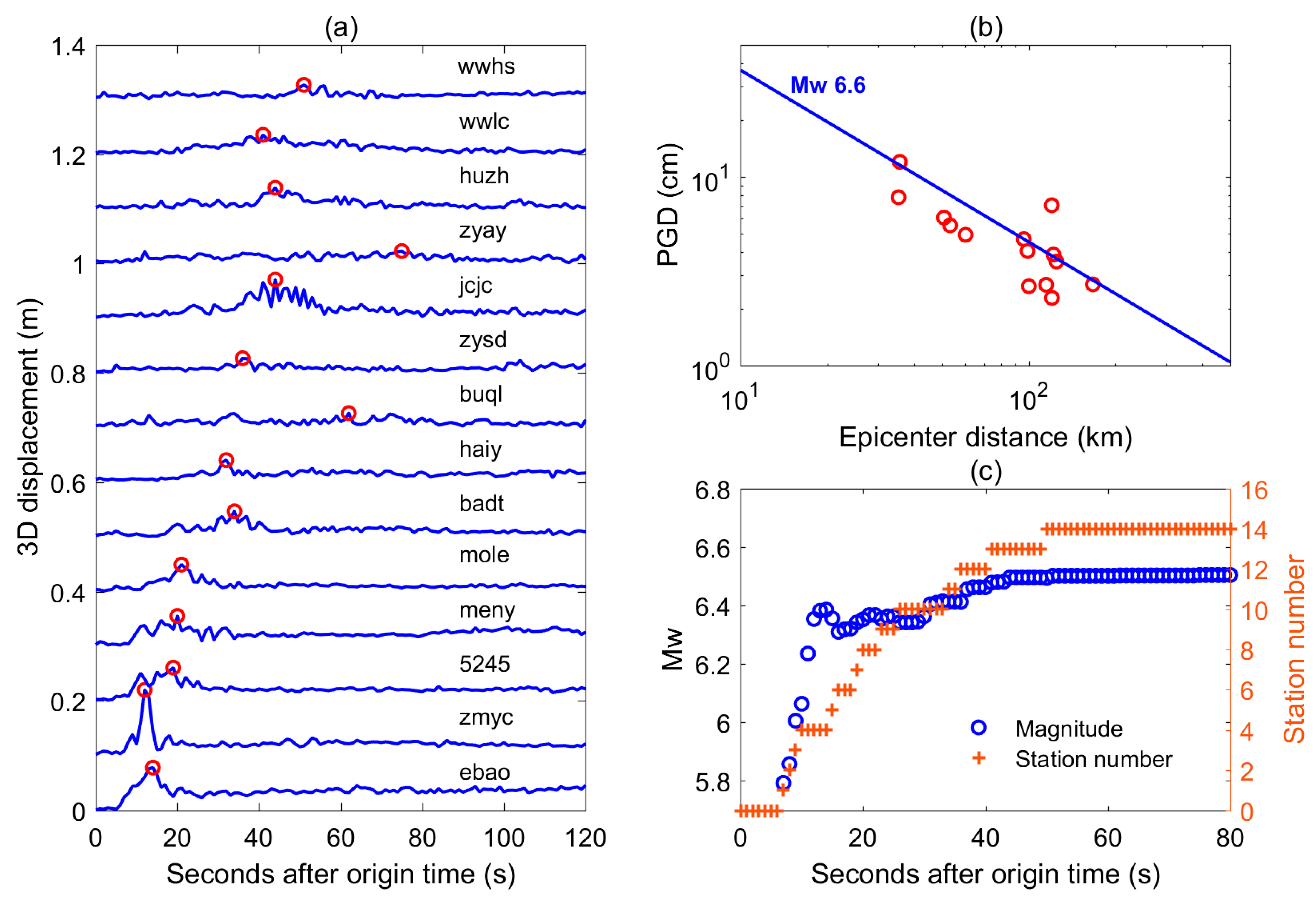
3.1. Warning Magnitude Calculation

Figure 2 presents the coseismic displacements of different GNSS stations processed with the RT-PPP. To calculate the real-time warning magnitude, the PGDs were retrieved at every epoch from the 3D coseismic displacements (Figure 3a). From the Figure 3b, we can observe that the final GNSS PGDs have a good agreement with the PGDs (blue line in Figure 3b) predicted by the regression relationship (2) with the known magnitude of Mw 6.6. The temporal evolution of the derived real-time warning magnitude estimates is presented in the Figure 3c, where the warning magnitude reaches Mw 6.0 at approximately 9 s when 4 stations are involved in the calculation, and exceeds Mw 6.2 at 11 s, and tends to be stable after approximately 45 s, the moment when most stations have already recorded the final PGDs (red circles in Figure 3a). The final stable magnitude calculated with the final PGDs of all GNSS stations is Mw 6.50, which is very close to the United States Geological Survey (USGS) magnitude of Mw 6.6.

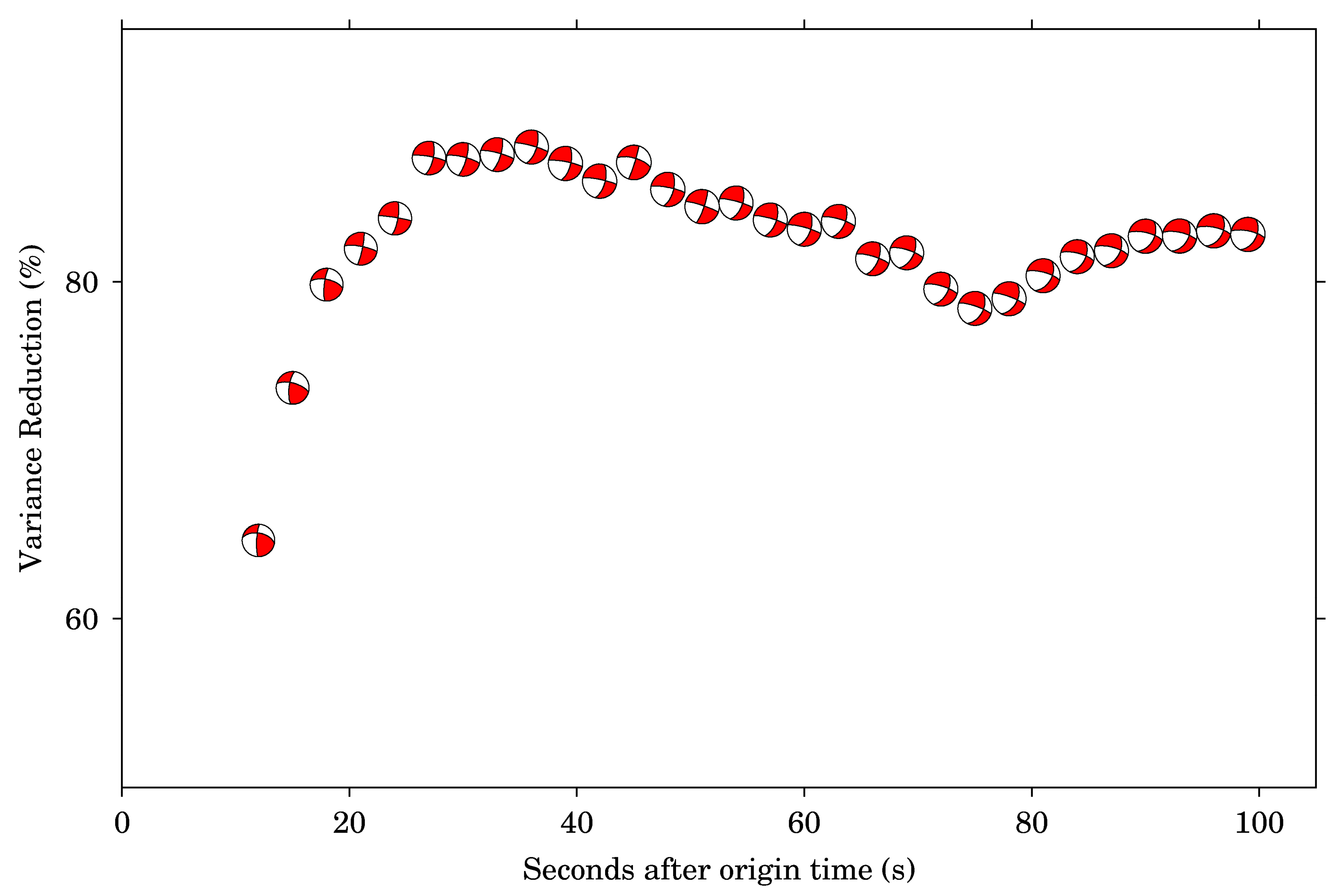
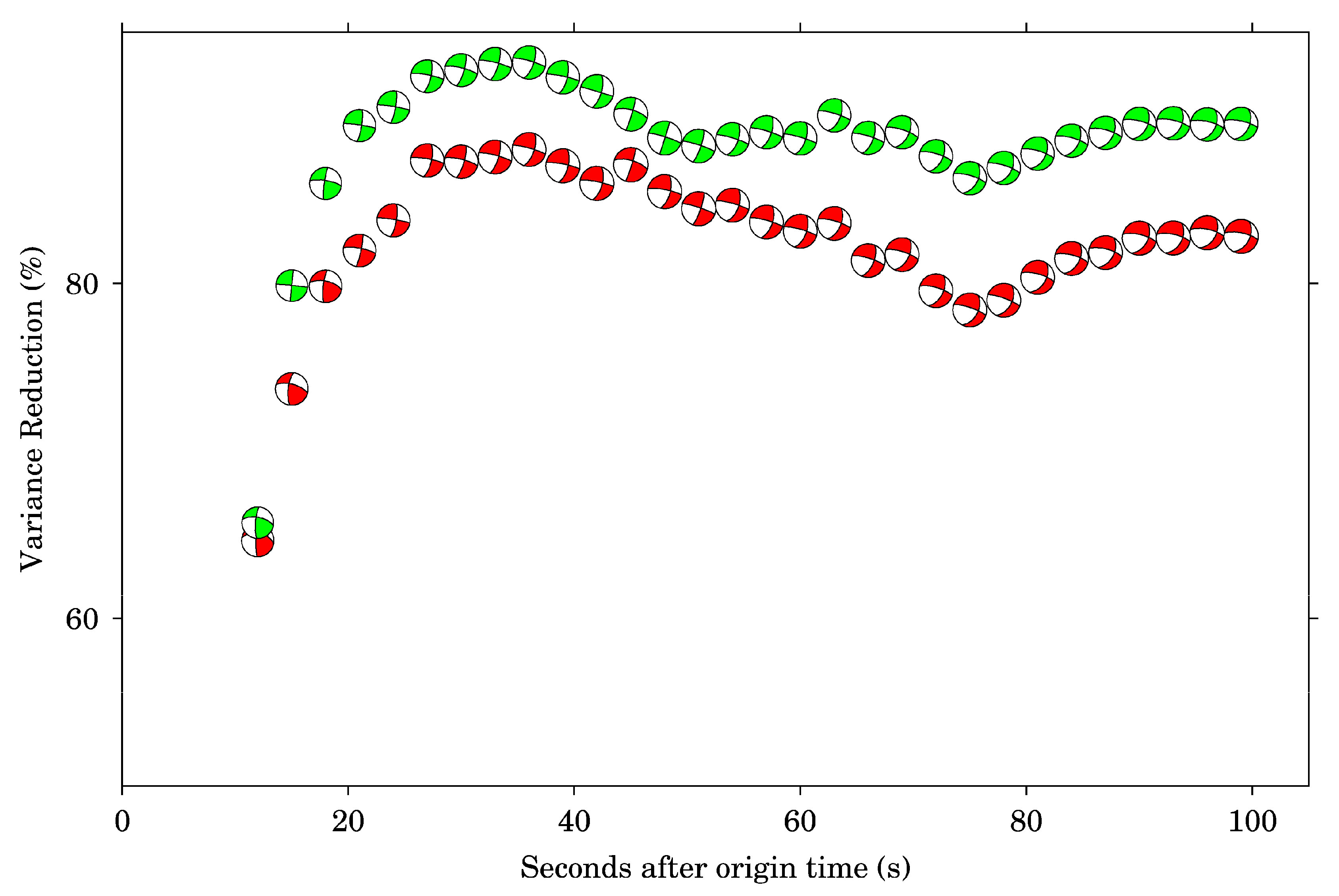
3.2. Centroid Moment Tensor Inversion

The centroid moment tensor inversion was performed at every epoch after the first warning magnitude available using the 30-s smoothed coseismic offsets (Figure 4). The derived focal mechanisms are demonstrated in the Figure 5, where it is observed that the variance reduction of the CMT result first exceeds 80% at approximately 20 s, and it also can be determined that the 2022 Menyuan earthquake is a strike-slip event after that time. The derived strikes, dips, and rakes at 21 s are 281°/80°/−8° and 12°/82°/−170° for the main and auxiliary fault planes, respectively, which are in general agreement with the results of Laboratoire de Détection et de Géophysique (CPPT) and Institut de Physique du Globe de Paris (IPGP). The derived nodal planes at 40 s, 60 s, 80 s and 100 s are listed in the

Table 1. Nodal planes derived from the inverted CMT results and the other agencies.

Solutions	Nodal Plane 1 Strike1°/Dip1°/Rake1°	Nodal Plane 2 Strike2°/Dip2°/Rake2°
USGS 1	104/88/15	13/75/178
GCMT 1	104/82/1	14/89/172
CPPT 1	285/84/−5	15/85/−174
GFZ 1	285/82/16	193/74/172
IPGP 1	284/89/−2	14/88/−179
fastCMT at 40 s	281/83/−24	15/66/−172
fastCMT at 60 s	285/80/−30	21/61/−168
fastCMT at 80 s	285/73/−43	30/50/−158
fastCMT at 100 s	282/73/−43	27/50/−157

¹ The nodal planes from USGS, GCMT, CPPT, Helmholtz-Centre Potsdam—German Research Centre for Geosciences (GFZ) and IPGP can be found at https://www.emsc-csem.org/Earthquake/tensors.php?view=42 (accessed on 2 September 2022).

, where we can observe that the strike 1 and dip 1 of the fastCMT results are in agreement with those of the CPPT and IPGP, while there are relatively large differences between the fastCMT results and CPPT and IPGP results in rake 1, dip2, and rake2.

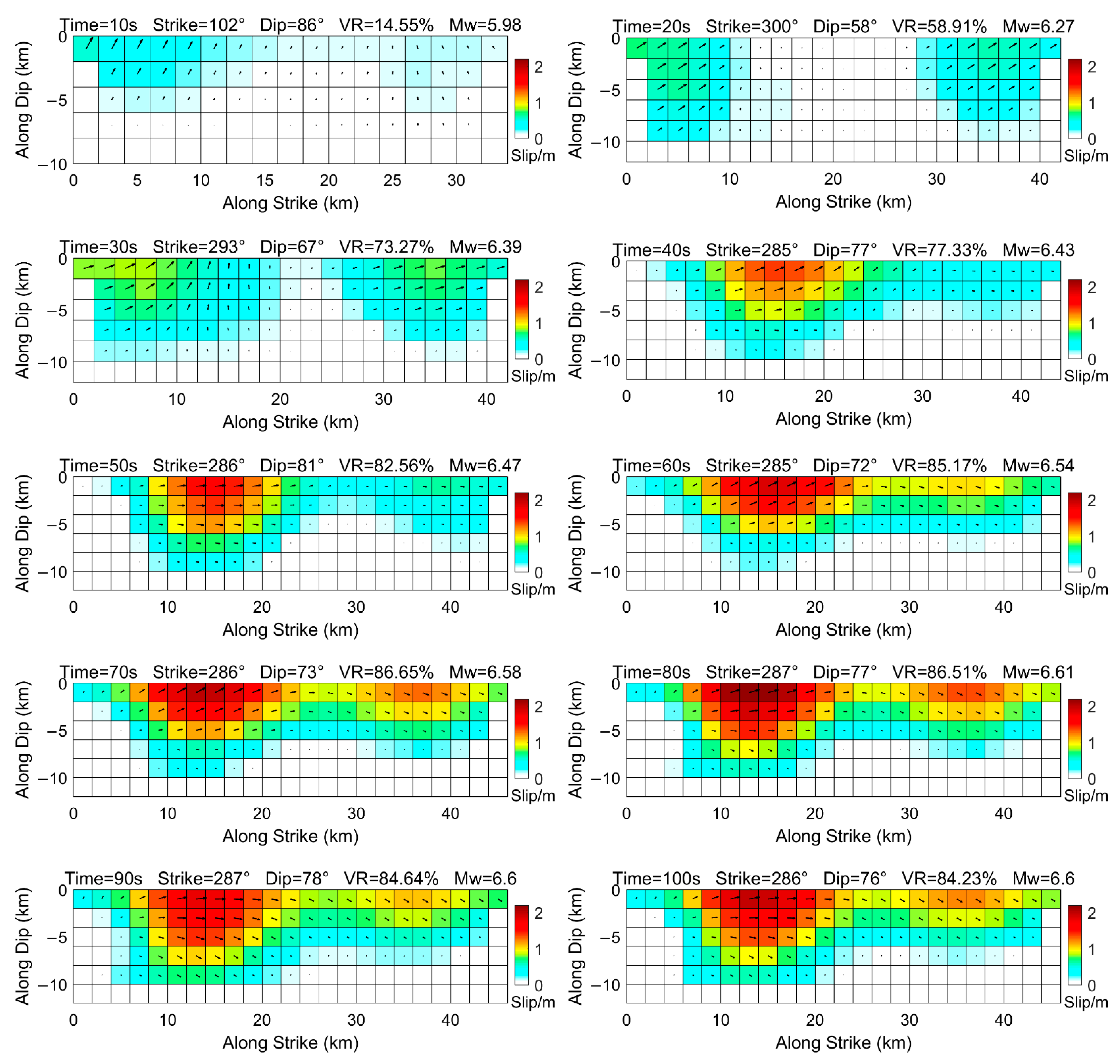
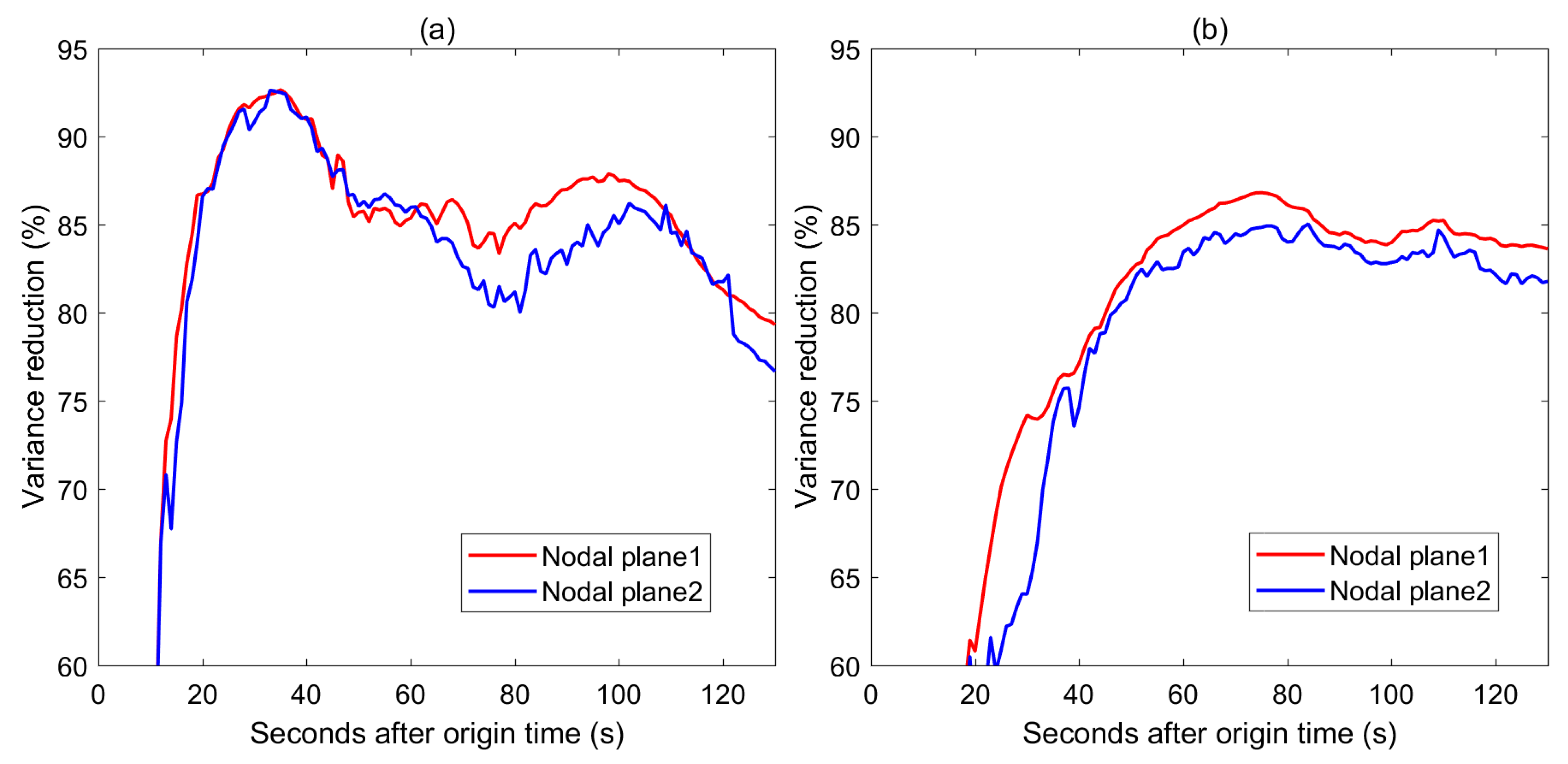
3.3. Static Fault Slip Distribution Inversion

Figure 6 portrays the inverted fault slips with an interval of 10 s on the nodal planes 1 using the 30-s smoothed coseismic offsets and the fault strikes and dips are from the inverted real-time CMT results. From Figure 6, the fault rupture spreads to the surface at approximately 20 s and the fault motion is mainly the left-lateral strike slip. With the increase of the coseismic offsets between 20 s and 40 s (Figure 4), the inverted fault slips also increase, and both the horizontal coseismic offsets and fault slips reach the maximum values at approximately 40 s. After 70 s of the earthquake, the inverted fault slips tend to be stable and the inverted maximum slips during this period vary between 1.3 m and 1.8 m with variance reduction changing between 83.66% and 87.88%; the moment magnitudes derived from these inverted slip models are from 6.64 to 6.67, which are in good agreement with the USGS result of Mw 6.6, InSAR-based inverted results of Mw 6.7 [48], and Mw 6.68 [49]. When comparing inverted slips of different times, it is observed that there are mainly two rupture areas in the inverted results of 20 s, 30 s, 70 s, 80 s, 90 s, and 100 s, which are different from the results of 40 s, 50 s, and 60 s. This is partly related to the variations of the fault strikes and dips. However, it should be noticed that all inverted slips after about 20 s show the obvious surface rupture, and the most fault motions are concentrated between the depth of 0 km and 8 km. The shallow fault slip characteristic of this earthquake might be responsible for the severe damage to infrastructures in the seismic areas.

4. Discussion

In the earthquake warning magnitude calculation, the accuracy of derived magnitude is strongly related to the coefficients of the regression relationship (2). In the past few years, several empirical relationships between the GNSS PGD and earthquake magnitude have been built [23,24,59]. Here, the performance of three empirical relationships for the 2022 Menyuan earthquake magnitude calculation was validated.

Table 2. Coefficients of three empirical regression relationships for the warning magnitude calculation.

Origin	A	B	C
Crowell et al., 2016 [59]	−6.687	1.500	−0.214
Melgar et al., 2015 [23]	−4.434	1.047	−0.138
Ruhl et al., 2018 [24]	−5.919	1.009	−0.145

lists the coefficients of the three relationships, and the derived magnitude estimates are presented in the Figure 7. It is observed that the changing processes of the derived magnitudes are similar for the three relationships, and all magnitude estimates tend to be stable after approximately 45 s. However, the magnitude values derived from the three relationships are obviously different. The finally stable magnitudes of the Ruhl relationship, Melgar relationship, and Crowell relationship are Mw 6.26, Mw 6.50, and Mw 6.75, respectively, and the differences between the final magnitudes and the USGS magnitude are −0.34, −0.10, and 0.15 for the three relationships. We can infer that the difference of the Ruhl relationship is larger than that of the other two relationships. Figure 8 compares the GNSS PGDs and PGDs predicted by the different empirical relationships, where it is observed that the GNSS PGDs have a good agreement with the PGDs predicted by the Melgar relationship. For the Crowell relationship, the GNSS PGDs follow the predicted line well when the epicenter distance is less than 80 km. However, for the Ruhl relationship, the GNSS PGDs are almost all below the predicted line, and thus resulting in an obviously low estimate of the magnitude for this earthquake.

In the centroid moment tensor inversion, the 1-D layered velocity structure was from the Crust 1.0, which is a global crustal model at 1 × 1 degrees. For comparison, we also performed the CMT inversion using the fastCMT method with 1-D layered velocity structure (

Table 3. 1-D layered velocity structure from Yin et al. [60].

Depth (km)	−3	0	5	10	15	20	25	35	45
Vp (km/s)	0.28	3.72	4.76	5.44	5.56	5.9	5.99	6.05	6.14
Vs (km/s)	0.36	2.77	2.67	3.34	3.41	3.07	3.63	3.74	4.05

) from Yin et al. [60], which is a local fine velocity structure model and was determined by the TomoDD method after the earthquake.

Figure 9 shows focal mechanisms derived from the CMT results inverted based on the different velocity structures, where the green focal mechanisms represent results inverted based on the Yin model and the red focal mechanisms denote results inverted based on the Crust 1.0. It is observed that although the VRs of the Yin model are higher than that of the Crust 1.0, the derived focal mechanisms of the two models are broadly like each other for most times. For example, the derived strikes, dips, and rakes at 100 s are 282°/76°/−40° and 24°/51°/−162° for the Yin model, which are in general agreement with the results of crust 1.0 with the values of 282°/73°/−43° and 27°/50°/−157°. In addition, it can be observed that the derived focal mechanisms are unstable after approximately 20 s from Figure 9, even though a local fine velocity structure model is used. This is mainly caused by the fluctuations of the 30-s smoothed coseismic offsets (Figure 4) and can be improved by increasing the length of smooth window. Figure 10 shows inverted focal mechanisms with coseismic offsets determined by averaging GNSS displacements with different smooth windows. The velocity structure used in these inversions is from the crust 1.0. It is observed that the VR of the 70-s window (blue) first exceeds 80% at approximately 40 s, which is later than that of the other two windows. However, the focal mechanisms of the 70-s window are more stable. This is because a relatively long smooth window can reduce more noise of the GNSS displacements.

In the fault slip distribution inversion, we find that the inverted fault slips are unstable (Figure 6), partly due to the variations of the fault planes built based on the real-time CMT results. When the fault plane is unchanged, the stable fault slips can be achieved quickly, even though 30-s smoothed coseismic offsets are used. Figure 11 shows fault slips inverted with the 30-s smoothed coseismic offsets on the fault plane built based on the focal mechanism of CPPT. It is observed that the inverted slip areas remain almost unchanged after approximately 40 s. However, in the earthquake early warning and the real-time source modeling, it is difficult to obtain the precise fault plane in advance. In comparison, the stability of the CMT inversion can be improved by using the coseismic offsets smoothed by a relatively long sliding window such as the case of blue focal mechanisms in Figure 10. Figure 12 shows fault slips inverted with the 70-s smoothed coseismic offsets on the fault planes built based on the CMT results, inverted with the same 70-s smoothed coseismic offsets. We can find that the main slip areas, between 10 km and 30 km along the strike, change little after the 40 s. However, it should be noticed that, compared with the fault slips inverted with the 30-s smoothed coseismic offsets (Figure 6), it takes a relatively long time to retrieve the first clear slip distribution in Figure 12.

In the above-mentioned fault slip distribution inversions, all fault planes were built based on the strikes and dips of the nodal planes 1. Indeed, CMT can be decomposed into two nodal planes. For the 2022 Menyuan earthquake, the nodal planes 1 were used because this earthquake occurred near the Lenglongling fault and the strikes of the nodal planes 1 are close to the strike of the Lenglongling fault. However, for some earthquakes, there is no known fault information in the seismic area. In such a case, the slip distribution inversions are performed on both two nodal planes and the nodal plane with the largest variance reduction is selected as the preferred fault plane. Figure 13 shows variance reductions of slip models inverted with the different coseismic offsets, where we can observe that it is difficult to determine the fault plane with the variance reduction when the 30-s smoothed coseismic offsets are used, because the variance reductions of the two nodal planes are comparable sometimes. In comparison, when the 70-s smoothed coseismic offsets are used, it is observed that the variance reductions of the nodal plane 1 are all greater than that of the nodal plane 2 after approximately 20 s.

5. Conclusions

In this study, the performance of 1 Hz GNSS on real-time warning magnitude calculation, centroid moment tensor inversion, and static fault slip distribution inversion was analyzed for the 2022 Mw 6.6 Menyuan earthquake. The accuracies of three empirical regression relationships for the magnitude calculation were validated and the results indicate that, compared with the USGS magnitude of Mw 6.6, the accuracy of Ruhl relationship is relatively low and the final stable magnitudes determined by the Melgar relationship and Crowell relationship are Mw 6.50 and Mw 6.75, respectively. With respect to the CMT inversion, the derived strikes, dips, and rakes at 21 s are close to the results of the CPPT and IPGP when the 30-s smoothed coseismic offsets are used. However, due to variations of the smoothed coseismic offsets, the variance reductions of the inverted CMT are unstable when 30-s smoothed coseismic offsets are used. Although the variance reduction of the inverted CMT can be improved by using a local fine velocity structure model, the derived focal mechanisms still are unstable. For the fault slip distribution inversion, the first clear fault slip distribution can be retrieved at about 20 s when the 30-s smoothed coseismic offsets are used. However, the derived fault slip areas vary over time partly due to the instability of the inverted focal mechanisms. When the 70-s smoothed coseismic offsets are used, the inverted fault slips are more stable, although the first clear fault slip distribution is retrieved until after approximately 40 s of the earthquake. In addition, we find that it is easier to identify the fault plane through the variance reductions of the two nodal planes when the 70-s smoothed coseismic offsets are used. However, it should be noticed that there are only 14 stations used in the CMT and fault slip distribution inversions in this earthquake. Whether the stability of the focal mechanism and fault slip, inverted with the 30-s smoothed coseismic offsets, can be improved when more near-field stations are used needs further investigation.

References

1. Wu, Y.; Zhao, L. Magnitude estimation using the first three seconds P-wave amplitude in earthquake early warning. Geophys. Res. Lett. 2006, 33, L16312. [Google Scholar] [CrossRef] [Green Version]
2. Zollo, A.; Lancieri, M.; Nielsen, S. Earthquake magnitude estimation from peak amplitudes of very early seismic signals on strong motion records. Geophys. Res. Lett. 2006, 33, L23312. [Google Scholar] [CrossRef]
3. Brown, H.; Allen, R.; Hellweg, M.; Khainovski, O.; Neuhauser, D.; Souf, A. Development of the ElarmS methodology for earthquake early warning: Realtime application in California and offline testing in Japan. Soil Dyn. Earthquake Eng. 2011, 31, 188–200. [Google Scholar] [CrossRef]
4. Larson, K.; Bodin, P.; Gomberg, J. Using 1-Hz GPS Data to Measure Deformations Caused by the Denali Fault Earthquake. Science 2003, 300, 1421–1424. [Google Scholar] [CrossRef] [PubMed] [Green Version]
5. Kouba, J. Measuring Seismic Waves Induced by Large Earthquakes with GPS. Stud. Geophys. Et Geod. 2003, 47, 741–755. [Google Scholar] [CrossRef]
6. Bock, Y.; Prawirodirdjo, L.; Melbourne, T. Detection of arbitrarily large dynamic ground motions with a dense high-rate GPS network. Geophys. Res. Lett. 2004, 31, L06604. [Google Scholar] [CrossRef] [Green Version]
7. Shi, C.; Lou, Y.; Zhang, H.; Zhao, Q.; Geng, J.; Wang, R.; Fang, R.; Liu, J. Seismic deformation of the Mw 8.0 Wenchuan earthquake from high-rate GPS observations. Adv. Space Res. 2010, 46, 228–235. [Google Scholar] [CrossRef] [Green Version]
8. Colosimo, G.; Crespi, M.; Mazzoni, A. Real-time GPS seismology with a stand-alone receiver: A preliminary feasibility demonstration. J. Geophys. Res. 2011, 116, B11302. [Google Scholar] [CrossRef] [Green Version]
9. Avallone, A.; Marzario, M.; Cirella, A.; Piatanesi, A.; Rovelli, A.; Di Alessandro, C.; D’Anastasio, E.; D’Agostino, N.; Giuliani, R.; Mattone, M. Very high rate (10 Hz) GPS seismology for moderate-magnitude earthquakes: The case of the Mw 6.3 L’Aquila (central Italy) event. J. Geophys. Res. 2011, 116, B02305. [Google Scholar] [CrossRef]
10. Ebinuma, T.; Kato, T. Dynamic characteristics of very-high-rate GPS observations for seismology. Earth Planets Space 2012, 64, 369–377. [Google Scholar] [CrossRef]
11. Xu, P.; Shi, C.; Fang, R.; Liu, J.; Niu, X.; Zhang, Q.; Yanagidani, T. High-rate precise point positioning (PPP) to measure seismic wave motions: An experimental comparison of GPS PPP with inertial measurement units. J. Geod. 2013, 87, 361–372. [Google Scholar] [CrossRef]
12. Lou, Y.; Zhang, W.; Shi, C.; Liu, J. High-rate (1-Hz and 50-Hz) GPS seismology: Application to the 2013 Mw 6.6 Lushan earthquake. J. Asian Earth Sci. 2014, 79, 426–431. [Google Scholar] [CrossRef]
13. Geng, T.; Xie, X.; Fang, R.; Su, X.; Zhao, Q.; Liu, G.; Li, H.; Shi, C.; Liu, J. Real-time capture of seismic waves using high-rate multi-GNSS observations: Application to the 2015 Mw 7.8 Nepal earthquake. Geophys. Res. Lett. 2016, 43, 161–167. [Google Scholar] [CrossRef] [Green Version]
14. Chen, K.; Ge, M.; Babeyko, A.; Li, X.; Diao, F.; Tu, R. Retrieving real-time co-seismic displacements using GPS/GLONASS: A preliminary report from the September 2015 Mw8.3 Illapel earthquake in Chile. Geophys. J. Int. 2016, 206, 941–953. [Google Scholar] [CrossRef] [Green Version]
15. Geng, J.; Jiang, P.; Liu, J. Integrating GPS with GLONASS for high-rate seismogeodesy. Geophys. Res. Lett. 2017, 44, 3139–3146. [Google Scholar] [CrossRef]
16. Shu, Y.; Fang, R.; Li, M.; Shi, C.; Li, M.; Liu, J. Very high-rate GPS for measuring dynamic seismic displacements without aliasing: Performance evaluation of the variometric approach. GPS Solut. 2018, 22, 121. [Google Scholar] [CrossRef]
17. Li, X.; Zheng, K.; Li, X.; Liu, G.; Ge, M.; Wickert, J.; Schuh, H. Real-time capturing of seismic waveforms using high-rate BDS, GPS and GLONASS observations: The 2017 Mw 6.5 Jiuzhaigou earthquake in China. GPS Solut. 2019, 23, 17. [Google Scholar] [CrossRef]
18. Zang, J.; Xu, C.; Chen, G.; Wen, Q.; Fan, S. Real-time coseismic deformations from adaptively tight integration of high-rate GNSS and strong motion records. Geophys. J. Int. 2019, 219, 1757–1772. [Google Scholar] [CrossRef]
19. Crowell, B. Near-Field Strong Ground Motions from GPS-Derived Velocities for 2020 Intermountain Western United States Earthquakes. Seismol. Res. Lett. 2021, 92, 840–848. [Google Scholar] [CrossRef]
20. Li, Z.; Ding, K.; Zhang, P.; Wen, Y.; Zhao, L.; Chen, J. Co-seismic deformation and slip distribution of 2021 Mw 7.4 madoi earthquake from GNSS observation. Geomat. Inf. Sci. Wuhan Univ. 2021, 46, 1489–1497. [Google Scholar] [CrossRef]
21. Zheng, K.; Liu, K.; Zhang, X.; Wen, G.; Chen, M.; Zeng, X.; Zhao, L.; He, X. First results using high-rate BDS-3 observations: Retrospective real-time analysis of 2021 Mw 7.4 Madoi (Tibet) earthquake. J. Geod. 2022, 96, 51. [Google Scholar] [CrossRef]
22. Crowell, B.; Melgar, D.; Bock, Y.; Haase, J.; Geng, J. Earthquake magnitude scaling using seismogeodetic data. Geophys. Res. Lett. 2013, 40, 6089–6094. [Google Scholar] [CrossRef]
23. Melgar, D.; Crowell, W.; Geng, J.; Allen, R.; Bock, Y.; Riquelme, S.; Hill, E.; Protti, M.; Ganas, A. Earthquake magnitude calculation without saturation from the scaling of peak ground displacement. Geophys. Res. Lett. 2015, 42, 5197–5205. [Google Scholar] [CrossRef]
24. Ruhl, C.; Melgar, D.; Geng, J.; Goldberg, D.; Crowell, B.; Allen, R.; Bock, Y.; Barrientos, S.; Riquelme, S.; Baez, J.; et al. A Global Database of Strong-Motion Displacement GNSS Recordings and an Example Application to PGD Scaling. Seismol. Res. Lett. 2019, 90, 271–279. [Google Scholar] [CrossRef] [Green Version]
25. Melgar, D.; Melbourne, T.; Crowell, B.; Geng, J.; Szeliga, W.; Scrivner, C.; Santillan, M.; Goldberg, D. Real-Time High-Rate GNSS Displacements: Performance Demonstration during the 2019 Ridgecrest, California, Earthquakes. Seismol. Res. Lett. 2020, 91, 1943–1951. [Google Scholar] [CrossRef]
26. Zang, J.; Xu, C.; Li, X. Scaling earthquake magnitude in real time with high-rate GNSS peak ground displacement from variometric approach. GPS Solut. 2020, 24, 101. [Google Scholar] [CrossRef]
27. Hodgkinson, K.; Mencin, D.; Feaux, K.; Sievers, C.; Mattioli, G. Evaluation of Earthquake Magnitude Estimation and Event Detection Thresholds for Real-Time GNSS Networks: Examples from Recent Events Captured by the Network of the Americas. Seismol. Res. Lett. 2020, 91, 1628–1645. [Google Scholar] [CrossRef]
28. Fang, R.; Zheng, J.; Geng, J.; Shu, Y.; Shi, C.; Liu, J. Earthquake Magnitude Scaling Using Peak Ground Velocity Derived from High-Rate GNSS Observations. Seismol. Res. Lett. 2021, 92, 227–237. [Google Scholar] [CrossRef]
29. Gao, Z.; Li, Y.; Shan, X.; Zhu, C. Earthquake Magnitude Estimation from High-Rate GNSS Data: A Case Study of the 2021 Mw 7.3 Maduo Earthquake. Remote Sens. 2021, 13, 4478. [Google Scholar] [CrossRef]
30. Melgar, D.; Bock, Y.; Crowell, B. Real-time centroid moment tensor determination for large earthquakes from local and regional displacement records. Geophys. J. Int. 2012, 188, 703–718. [Google Scholar] [CrossRef]
31. O’Toole, T.; Valentine, A.; Woodhouse, J. Earthquake source parameters from GPS-measured static displacements with potential for real-time application. Geophys. Res. Lett. 2013, 40, 60–65. [Google Scholar] [CrossRef] [Green Version]
32. Minson, S.; Murray, J.; Langbein, J.; Gomberg, J. Real-time inversions for finite fault slip models and rupture geometry based on high-rate GPS data. J. Geophys. Res. Solid Earth 2014, 119, 3201–3231. [Google Scholar] [CrossRef]
33. Zhang, Y.; Wang, R.; Zschau, J.; Chen, Y.; Parolai, S.; Dahm, T. Automatic imaging of earthquake rupture processes by iterative deconvolution and stacking of high-rate GPS and strong motion seismograms. J. Geophys. Res. Solid Earth 2014, 119, 5633–5650. [Google Scholar] [CrossRef] [Green Version]
34. Allen, R.; Ziv, A. Application of real-time GPS to earthquake early warning. Geophys. Res. Lett. 2011, 38, L16310. [Google Scholar] [CrossRef]
35. Ohta, Y.; Kobayashi, T.; Tsushima, H.; Miura, S.; Hino, R.; Takasu, T.; Fujimoto, H.; Iinuma, T.; Tachibana, K.; Demachi, T.; et al. Quasi real-time fault model estimation for near-field tsunami forecasting based on RTK-GPS analysis: Application to the 2011 Tohoku-Oki earthquake (Mw 9.0). J. Geophys. Res. Solid Earth 2012, 117, B02311. [Google Scholar] [CrossRef]
36. Colombelli, S.; Allen, R.; Zollo, A. Application of real-time GPS to earthquake early warning in subduction and strike-slip environments. J. Geophys. Res. Solid Earth 2013, 118, 3448–3461. [Google Scholar] [CrossRef] [Green Version]
37. Grapenthin, R.; Johanson, I.; Allen, R. Operational real-time GPS-enhanced earthquake early warning. J. Geophys. Res. Solid Earth 2014, 119, 7944–7965. [Google Scholar] [CrossRef]
38. Crowell, B.; Melgar, D.; Geng, J. Hypothetical Real-Time GNSS Modeling of the 2016 Mw 7.8 Kaikōura Earthquake: Perspectives from Ground Motion and Tsunami Inundation Prediction. Bull. Seismol. Soc. Am. 2018, 108, 1736–1745. [Google Scholar] [CrossRef]
39. Zang, J.; Xu, C.; Wen, Y.; Wang, X.; He, K. Rapid earthquake source description using Variometric-derived GPS displacements towards application to the 2019 Mw 7.1 Ridgecrest earthquake. Seismol. Res. Lett. 2022, 93, 56–67. [Google Scholar] [CrossRef]
40. Zang, J.; Wen, Y.; Li, Z.; Xu, C.; He, K.; Zhang, P.; Wen, G.; Fan, S. Rapid source models of the 2021 Mw 7.4 Maduo, China, earthquake inferred from high-rate BDS3/2, GPS, Galileo and GLONASS observations. J. Geod. 2022, 96, 58. [Google Scholar] [CrossRef]
41. Xu, X.; Yeats, R.; Yu, G. Five Short Historical Earthquake Surface Ruptures near the Silk Road, Gansu Province, China. Bull. Seismol. Soc. Am. 2010, 100, 541–561. [Google Scholar] [CrossRef]
42. Guo, P.; Han, Z.; Jiang, W.; Mao, Z. Holocene Left-Lateral Slip Rate of the Lenglongling Fault, Northeastern Margin of the Tibetan Plateau. Seismol. Geol. 2017, 39, 323–341. [Google Scholar] [CrossRef]
43. He, X.; Zhang, Y.; Shen, X.; Zheng, W.; Zhang, P.; Zhang, D. Examination of the Repeatability of Two Ms6.4 Menyuan Earthquakes in Qilian-Haiyuan Fault Zone (NE Tibetan Plateau) Based on Source Parameters. Phys. Earth Planet. Inter. 2020, 299, 106408. [Google Scholar] [CrossRef]
44. Pan, J.; Li, H.; CHEVALIER, M.; Liu, D.; Li, C.; Liu, F.; Wu, Q.; Lu, H.; Jiao, L. Coseismic Surface Ruptures and Seismogenic structure of the 2022 Ms6.9 Menyuan Earthquake, Qinghai Province. China. Acta Geol. Sin. 2022, 96, 215–231. [Google Scholar] [CrossRef]
45. Li, Z.; Gai, H.; Li, X.; Yuan, D.; Xie, H.; Jiang, W.; Li, Y.; Su, Q. Seismogenic Fault and Coseismic Surface Deformation of the Menyuan Ms6.9 Earthquake in Qinghai. China Acta Geol. Sin. 2022, 96, 330–335. [Google Scholar] [CrossRef]
46. Yang, H.; Wang, D.; Guo, R.; Xie, M.; Zang, Y.; Wang, Y.; Yao, Q.; Cheng, C.; An, Y.; Zhang, Y. Rapid Report of the 8 January 2022 Ms6.9 Menyuan Earthquake, Qinghai, China. Earthq. Res. Adv. 2022, 2, 100113. [Google Scholar] [CrossRef]
47. Liu, J.; Hu, J.; Li, Z.; Ma, Z.; Shi, J.; Xu, W.; Sun, Q. Three-Dimensional Surface Displacements of the 8 January 2022 Mw6.7 Menyuan Earthquake, China from Sentinel-1 and ALOS-2 SAR Observations. Remote Sens. 2022, 14, 1404. [Google Scholar] [CrossRef]
48. Li, Z.; Han, B.; Liu, Z.; Zhang, M.; Yu, C.; Chen, B.; Liu, H.; Du, J.; Zhang, S.; Zhu, W.; et al. Source Parameters and Slip Distributions of the 2016 and 2022 Menyuan, Qinghai Earthquakes Constrained by InSAR Observations. Geomat. Inf. Sci. Wuhan Univ. 2022, 47, 887–897. [Google Scholar] [CrossRef]
49. Feng, W.; He, X.; Zhang, Y.; Fang, L.; Samsonov, S.; Zhang, P. Seismic Faults of the 2022 Mw6.6 Menyuan, Qinghai Earthquake and Their Implication for the Regional Seismogenic Structures. Chin. Sci. Bull. 2022. [Google Scholar] [CrossRef]
50. Fan, L.; Li, B.; Liao, S.; Jiang, C.; Fang, L. Precise Earthquake Sequence Relocation of the January 8, 2022, Qinghai Menyuan Ms6.9 Earthquake. Earthq. Sci. 2022, 35, 138–145. [Google Scholar] [CrossRef]
51. Liu, Z.; Zhang, G.; Liang, S.; Zou, L. Spatial Migration Characteristics of the Aftershock Sequence of the Menyuan, Qinghai Ms6.9 Earthquake in 2022. Chin. Earthq. Eng. J. 2022, 44, 475–487. [Google Scholar] [CrossRef]
52. Xu, Y.; Guo, X.; Feng, L. Relocation and Focal Mechanism Solutions of the MS6.9 Menyuan Earthquake Sequence on January 8, 2022 in Qinghai Province. Acta Seismol. Sin. 2022, 44, 195–210. [Google Scholar] [CrossRef]
53. Zumberge, J.; Heflin, M.; Jefferson, D.; Watkins, M.; Webb, F. Precise point positioning for the efficient and robust analysis of GPS data from large networks. J. Geophys. Res. 1997, 102, 5005–5017. [Google Scholar] [CrossRef] [Green Version]
54. Boehm, J.; Niell, A.; Tregoning, P.; Schuh, H. Global Mapping Function (GMF): A New Empirical Mapping Function Based on Numerical Weather Model Data. Geophys. Res. Lett. 2006, 33, L07304. [Google Scholar] [CrossRef] [Green Version]
55. Kouba, J. A Guide to Using International GNSS Service (IGS) Products. Available online: https://kb.igs.org/hc/en-us/articles/201271873-A-Guide-to-Using-the-IGS-Products (accessed on 2 September 2022).
56. Wang, R.; Martin, F.; Roth, F. Computation of deformation induced by earthquakes in a multi-layered elastic crust: FORTRAN programs EDGRN/EDCMP. Comput. Geosci. 2003, 29, 195–207. [Google Scholar] [CrossRef]
57. Wells, D.; Coppersmith, K. New empirical relationships among magnitude, rupture length, rupture width, rupture area, and surface displacement. Bull. Seismol. Soc. Am. 1994, 84, 974–1002. [Google Scholar] [CrossRef]
58. Okada, Y. Surface deformation due to shear and tensile faults in a half-space. Bull. Seismol. Soc. Am. 1985, 75, 1135–1154. [Google Scholar] [CrossRef]
59. Crowell, B.; Schmidt, D.; Bodin, P.; Vidale, J.; Gomberg, J.; Renate Hartog, J.; Kress, V.; Melbourne, T.; Santillan, M.; Minson, S.; et al. Demonstration of the Cascadia G-FAST geodetic earthquake early warning system for the Nisqually, Washington, earthquake. Seismol. Res. Lett. 2016, 87, 930–943. [Google Scholar] [CrossRef]
60. Yin, X.; Qiu, J.; Li, M.; Xu, K.; Zhang, B.; Zhang, S. Three-dimensional velocity structure and seismogenic mechanism of Menyuan MS6.9 earthquake in 2022. Chin. Earthq. Eng. J. 2022, 44, 360–369. [Google Scholar] [CrossRef]
Figure 2. Coseismic displacements of all GNSS stations during the 2022 Mw 6.6 Menyuan earthquake. For the clarity, the displacements of different stations are offset in the vertical axis.
Remotesensing 14 05378 g002
Figure 3. (a) 3D coseismic displacements of all GNSS stations during the 2022 Mw 6.6 Menyuan earthquake. The red circles represent the final PGDs. For the clarity, the 3D coseismic displacements of different GNSS stations are offset in the vertical axis. (b) The final GNSS PGDs with the epicenter distance. The blue oblique line is the predicted PGDs from the regression relationship (2) with the known magnitude of Mw 6.6. (c) Temporal evolution of the derived warning magnitude estimates. The red crosses represent the number of stations involved in the magnitude calculation at each epoch.
Remotesensing 14 05378 g003
Figure 4. 30-s smoothed coseismic offsets of all GNSS stations during the 2022 Mw 6.6 Menyuan earthquake.
Remotesensing 14 05378 g004
Figure 5. Focal mechanisms derived from the CMT results inverted with the 30-s smoothed coseismic offsets.
Remotesensing 14 05378 g005
Figure 6. The fault slips inverted with the 30-s smoothed coseismic offsets. The distance along the strike increases from west to east.
Remotesensing 14 05378 g006
Figure 7. Temporal evolutions of the magnitude estimates determined by the Ruhl relationship, Melgar relationship, and Crowell relationship, respectively.
Remotesensing 14 05378 g007
Figure 8. GNSS PGDs with the epicenter distance. The oblique lines are the predicted PGDs from the regression relationship of Melgar (green), Crowell (blue), and Ruhl (black) with the known magnitude of Mw 6.6.
Remotesensing 14 05378 g008
Figure 9. The comparison of focal mechanisms derived from the CMT results inverted based on the crust 1.0 (red) and a local fine velocity structure model (green) using the 30-s smoothed coseismic offsets.
Remotesensing 14 05378 g009
Figure 10. The comparison of the focal mechanisms derived from the CMT results inverted with the 30-s smoothed coseismic offsets (red), 50-s smoothed coseismic offsets (green), and 70-s smoothed coseismic offsets (blue).
Remotesensing 14 05378 g010
Figure 11. The fault slips inverted with the 30-s smoothed coseismic offsets and the fault strike and dip are from the focal mechanism of CPPT. The distance along the strike increases from west to east.
Remotesensing 14 05378 g011
Figure 12. The fault slips inverted with the 70-s smoothed coseismic offsets. The distance along the strike increases from west to east.
Remotesensing 14 05378 g012
Figure 13. (a) Variance reductions of the fault slips inverted on the two nodal planes using the 30-s smoothed coseismic offsets (b) Variance reductions of the fault slips inverted on the two nodal planes using the 70-s smoothed coseismic offsets.
Remotesensing 14 05378 g013