DSANet: A Deep Supervision-Based Simple Attention Network for Efficient Semantic Segmentation in Remote Sensing Imagery

Abstract

Semantic segmentation for remote sensing images (RSIs) plays an important role in many applications, such as urban planning, environmental protection, agricultural valuation, and military reconnaissance. With the boom in remote sensing technology, numerous RSIs are generated; this is difficult for current complex networks to handle. Efficient networks are the key to solving this challenge. Many previous works aimed at designing lightweight networks or utilizing pruning and knowledge distillation methods to obtain efficient networks, but these methods inevitably reduce the ability of the resulting models to characterize spatial and semantic features. We propose an effective deep supervision-based simple attention network (DSANet) with spatial and semantic enhancement losses to handle these problems. In the network, (1) a lightweight architecture is used as the backbone; (2) deep supervision modules with improved multiscale spatial detail (MSD) and hierarchical semantic enhancement (HSE) losses synergistically strengthen the obtained feature representations; and (3) a simple embedding attention module (EAM) with linear complexity performs long-range relationship modeling. Experiments conducted on two public RSI datasets (the ISPRS Potsdam dataset and Vaihingen dataset) exhibit the substantial advantages of the proposed approach. Our method achieves 79.19% mean intersection over union (mIoU) on the ISPRS Potsdam test set and 72.26% mIoU on the Vaihingen test set with speeds of 470.07 FPS on 512 × 512 images and 5.46 FPS on 6000 × 6000 images using an RTX 3090 GPU.

1. Introduction

Remote sensing is a crucial technical tool for large-scale observations of the Earth’s surface. With the rapid development of Earth observation and remote sensing imaging technology, remote sensing has entered the era of big data [1]. Big data qualities for remote sensing primarily involve three Vs: volume, velocity, and variety of data [2]. Every day, a massive volume of remote sensing data must be handled in the era of big data for remote sensing. Furthermore, increasingly diverse remote sensing data are playing important roles in several fields. Due to advances in imaging technology, very high-resolution (VHR) imagery has shown considerable potential in remote sensing images (RSIs) interpretation and has been the focus of semantic segmentation.

Semantic segmentation is a critical task in computer vision, and its special application to remote sensing is RSI interpretation. It requires pixelwise parsing of the input image to retrieve the predefined categories to which the elements belong. Semantic segmentation has broad and vital applications in a variety of fields. This is especially true in the realm of remote sensing, where subjects such as integrated land use and land cover mapping [3,4], town change detection [5,6], urban functional areas [7], building footprints [8], impervious surfaces [9], and water body [10] extraction. The majority of these applications and methodologies are based on VHR images and are constrained by the two issues listed below. (1) Information modeling with little detail. In comparison to prior low-resolution images, VHR images give unequal spatial and semantic information volume gains. The significant improvement in spatial resolution allows for the observation of previously unseen features. However, vital detail information is mixed in with a vast volume of redundant information, providing additional obstacles for information extraction. (2) Inefficient processing. On the data processing front, high-resolution imagery implies that the amount of data to be processed per unit of observation area for interpretation is rising dramatically, posing a considerable challenge for hardware and algorithms.

Researchers have proposed numerous ways to overcome the difficulties of semantic segmentation for VHR images in the age of big data. Deep learning algorithms are the primary techniques for semantic segmentation at the moment. Unlike classic machine learning algorithms based on prior knowledge and predetermined rules, deep learning algorithms are data-driven algorithms that perform poorly with tiny data samples but may be utilized to great advantage in the era of big data. Deep learning-based convolutional neural networks (CNNs) outperform classic machine learning methods in terms of performance. Fully convolutional networks (FCNs) [11] have been utilized to obtain outstanding results in the semantic segmentation of RSIs. Following study, numerous model variants based on the FCN architecture have been developed, making substantial advances in various aspects. UNet [12], which is based on an encoder-decoder architecture, enhances the FCN’s capacity to represent the multiscale features of images through contraction paths and expansion paths for achieving high-precision road [13] and coastline recognition [14] in RSIs. The DeepLabv3 series [15,16] utilize parallelized atrous spatial pyramid pooling (ASPP) with varying ratios to expand the models’ reception fields while obtaining multiscale features; these models are widely used in RSI semantic segmentation, cloud detection [17], etc. However, because to the poor inference speeds of these models and the high hardware needs placed on deployed devices, these approaches find it difficult to overcome the aforementioned two problems. Figure 1 depicts the problem of building segmentation models that take both efficiency and performance into account.

In addition to investigating model segmentation performance, another approach is to optimize the efficiency and accelerate the inference speed of the utilized model. A conceivable way to accomplish lightweight model building is to reduce the number of model channels and add an attention mechanism to compensate for the loss in model performance [18]. In addition to incorporating an attention module, the introduction of a deep supervision [19] module can also enhance the segmentation performance of the model. By actively monitoring the body and edge characteristics of the object of interest, a lightweight semantic segmentation network was suggested to maximize the overall consistency and object details of semantic segmentation results [20]. Loss functions expressly designed for the semantic segmentation task can speed up the learning process of the resultant model for fundamental spatial information such as borders [21] and spatial correlations [22], as evidenced by higher performance with the same amount of training epochs. These lightweight networks struggle to capture the rich, detailed aspects of VHR images with fewer parameters, reducing accuracy significantly.

We investigate a solution for alleviating data interpretation burden in the era of large data for remote sensing that balances performance and inference speed. The functions of a lightweight network backbone, an attention mechanism, a deep supervision module, and a loss function in attaining effective semantic segmentation are thoroughly investigated in this paper. Our contributions are summarized here.

(1)

To alleviate the VHR images interpretation mistake in the age of large data, an efficient deep-layer and shallow-channel network with spatial and semantic enhancement losses (DSANet) is developed.

(2)

Without inference speed costs, two multiscale feature losses are proposed: improved multiscale spatial detail (MSD) and hierarchical semantic enhancement (HSE). The MSD loss is intended to improve the model’s extraction of underlying spatial information, whilst the HSE loss assists the model in understanding the observed distribution of categories.

(3)

The addition of the embedding attention module (EAM) decreases the attention module’s complexity from quadratic (self-attention) to linear with equivalent accuracy, as well as increasing inference speed for large images.

(4)

On the ISPRS Potsdam and Vaihingen benchmark data-sets, we attain outstanding results. Using an RTX 3090 GPU, we achieve mean intersection over unions (mIoUs) of 79.19% on the Potsdam test set and 72.26% on the Vaihingen test set, with a speed of 470.07 frames per second (FPS) on 512 × 512 images and 5.46 FPS on 6000 × 6000 images.

The rest of this paper is organized as follows. Section 2 reviews related works involving efficient network designs, efficient semantic segmentation approaches, information enhancement modules, and attention mechanisms. Section 3 presents the network structure of the proposed model and the detailed principles of its modules. Section 4 introduces the utilized datasets and demonstrates the implementation details of our experiments. The ablation experiments and a results comparison with state-of-the-art methods are also included in Section 5. Finally, Section 6 provides a summary of the paper.

2. Related Works

Many lightweight segmentation algorithms have obtained impressive results on many benchmarks in the domains of autonomous driving, video surveillance, and VHR remote sensing scene perception in the last 5–10 years. This section reviews efficient network designs and related works, categorizing them as follows: efficient network designs, efficient semantic segmentation approaches, information enhancement modules, and attention mechanisms.

2.1. Efficient Network Designs

Researchers are discovering that network design is becoming increasingly crucial as the Visual Geometry Group network (VGGNet) [23], the residual network (ResNet) [24], and DenseNet [25] models continue to be suggested. Because semantic segmentation is a dense prediction task, related models tend to have more parameters and slower inference speeds, which is harmful to model deployment and severely limits their application possibilities. An efficient network design paradigm lends itself well to the creation of efficient segmentation networks. By extensively replacing the 3 × 3 convolution in the model with a 1 × 1 convolution and reducing the number of channels in the 3 × 3 convolution, SqueezeNet [26] achieves comparable classification accuracy to AlexNet [27] with 2% of the total parameters. The MobileNet series [28,29,30] has steadily introduced new techniques to deep separable networks such as inverted residuals and neural architecture search (NAS). By integrating group convolution and channel shuffling operations and employing four recommendations, the ShuffleNet series [31,32] achieves a balance between accuracy and parameter number. 1. Equal channel widths minimize the memory access cost (MAC). 2. Excessive group convolution increases the MAC. 3. Network fragmentation reduces the degree of parallelism. 4. Elementwise operations are nonnegligible. Several outstanding and efficient semantic segmentation models have been presented as a result of these exploratory efforts on efficient network construction.

2.2. Efficient Semantic Segmentation Methods

Efficient semantic segmentation models strive for a balance between accuracy and speed, with considerable inference speed benefits at a low accuracy cost. They represent a significant development in the field of semantic segmentation in terms of efficiency, and they have created many good works based on the collaborative efforts of scholars. The two dominant approaches point the way to achieving high-accuracy and efficient semantic segmentation. 1. Light-weight backbones. ENet [33], a representative of earlier efficient segmentation models, greatly reduces the number of required parameters and floating point operations (FLOPs) by employing an asymmetric encoder-decoder structure and factorizing filters. Subsequent work has focused on asymmetric networks, with the goal of improving model performance by using deeply separable convolutions [34], dilated convolutions [35], factorized convolutions [36,37], dense connections [38], skip connections [39], pyramidal pooling [40] and channel splitting and shuffling [41]. The Fast-shallow CNN (SCNN) [42] adopts shared shallow network paths to encode details while learning contexts at low resolutions, saving computing costs. STDCNet [38] utilizes a lightweight backbone network from DenseNet with layer concatenation. Dual-resolution branch networks [43], exemplified by the bilateral segmentation network (BiSeNet) series [44,45], provide effective segmentation by modifying extraction branches for spatial and semantic information independently. 2. Feature aggregation. The deep feature aggregation network (DFANet) [46] recommends two deep branches where several bilateral fusions are conducted. By steering upper-level feature upsampling using low-level features, SFNet [47] achieves higher-resolution restoration and cross-layer feature aggregation. DDRNet [48] advises two deep branches between which multiple bilateral fusions are performed.

2.3. Information Enhancement Modules

The information in computer vision tasks can be divided into spatial and semantic information, both of which contribute significantly to accurate segmentation. (1) Enhancing spatial information. Typically, the shallow layer of the encoder may better describe spatial information. Ensuring that a branch has a high resolution preserves spatial information to the greatest extent possible. STDCNet adopts the Laplacian kernel of the pyramid hierarchy as an auxiliary loss function, which expedites the process of learning spatial edge features. Researchers suggest that the quantifications and statistics of spatial texture aspects are likewise of great significance due to quantization and counting operators. (2) Enhancing semantic information. PSPNet [49] adopts pyramid pooling to enhance the observed multiscale semantic features. The DeepLab series [15,16,50,51] utilizes parallel atrous convolutions with varying dilation rates; this approach is called ASPP, which can encode multiscale semantic information more effectively. DANet [52] models long-range dependencies in the channels and positions of sematic features using a dual self-attention module. OCRNet [53] explicitly turns the pixel classification problem into an object area classification problem, computes the relationship between each pixel and each object region, and augments the representation of each pixel with an object-contextual representation.

2.4. Attention Mechanisms

The selected attention mechanism is a crucial component of model design and is a key module for improving model performance. It is a descriptive weighting of the relationship between a particular attribute (from a small pixel value to an entire channel) and the data, so that it can be chosen to suppress or amplify that attribute at a particular location in order to achieve a selective representation of a particular feature for the model. The outstanding early approach is the squeeze-and-excitation network (SENet) [54], which squeezes the features on each channel by global maximum pooling and uses a fully connected layer to encode the features into a low-dimensional space before performing decoding. This makes the SENet an excellent attention module without imposing many additional parameters or a large computational burden on the subject network. The SENet’s concept of squeezing and extracting channels and examining spatial attention inspired further research. Important follow-ups include the block attention module (BAM) [55] and convolutional BAM (CBAM) [56]. A BAM includes a two-branch parallel attention computation paradigm, with channel attention branches that adhere to the SENet’s approach. Spatial features are squeezed in the channel dimension by a 1 × 1 convolution, key spatial features are extracted using a 3 × 3 convolution, and finally, a pixelwise summation operation is performed for both attention weights. A CBAM selects a multistep attention paradigm that combines channel attention and spatial attention simultaneously. The combination of spatial attention with gated mechanisms is another way to utilize attention mechanisms [57]. Unlike the idea of feature compression and extraction in the above work, self-attention [58] is a pixel-level attention mechanism. The computational complexity and resource needs of this method are an order of magnitude more than those of the preceding approaches, despite the fact that its performance is superior. Transformers [59], which outperform CNNs in many tasks, are excellent models based on self-attention; however, researchers are still designing optimizations for visual tasks such as patches [60] and hierarchical architectures [61,62] to overcome the fatal flaw of a computationally intensive attention mechanism. Fortunately, self-attention based on queries, keys and values can be optimized from O(n2) complexity to linear complexity by changing the order of computation [63], performing approximate computation [64], and conducting low-rank singular value decomposition [65].

It is typical practice for effective semantic segmentation networks [33,44] to utilize an attention module based on the SENet or linear simplified self attention due to its computational efficiency and inference speed.

3. Methodology

Our proposed segmentation model (DSANet) adheres to the original design concepts outlined below: (1) to adhere to Occam’s razor: entities should not be multiplied beyond necessity; (2) to have the smallest possible number of parameters while obtaining acceptable accuracy; and (3) to avoid modules that improve the model’s representation capabilities but consume an unacceptable amount of time during inference. Important aspects of the model include: (1) its low channel capacity and extra downsampling stages in the backbone to quickly obtain large perceptual fields, (2) the combined multiscale spatial detail loss and hierarchical semantic enhancement loss in the deep supervision module, and (3) a simple attention module with linear complexity. The details of DSANet can be seen in Figure 2.

3.1. Network Architecture of the Proposed Method

DSANet is an asymmetric, U-shaped, basic network with an encoder for the contracting path and a decoder for the expansion path.

In contrast to prior lightweight semantic segmentation networks that employ two-branch designs, i.e., semantic and spatial branches, we employ a single backbone branch that is anticipated to extract both spatial and semantic information. For such single-branch networks, it is essential to improve spatial feature extraction. Good spatial texture information and color information are required for the model to sense semantics, and correct boundary detail information is essential for directing the high-resolution reconstruction of semantic components. Observing the inference time spent by BiSeNet (see details in

Table 1. Analysis of the Number of Parameters, Number of Computations and Inference Time of the BiSeNet Network.

Module	Params (M)	FLOPs (G)	Inference Time (ms)
SP	0.685	9.586	3.84
ARM32	4.521	1.023	0.74
ARM16	2.323	2.048	21.94
FFM	0.984	1.836	4.56
All	8.513	14.493	31.08

Note that all data are in percentages. ARM32 and ARM16 represent ARM applied to 1/32 and 1/16 scales, respectively.

) reveals that (1) the spatial path (SP) for extracting spatial information, the attention refinement module (ARM) for refining semantic features, and the feature fusion module (FFM) for feature interaction account for more than 30% of the model inference speed; (2) performing feature operations at the second-to-last scale (ARM16) is extremely time-consuming and unsatisfactory.

To reduce the number of parameters in the model, including the number of layers and channel capacities, are redesigned. A typical semantic segmentation task only downsamples an image to 1/16 or 1/32 through the encoder and performs operations such as feature refinement and attention at this scale; this is totally insufficient for VHR images. Our method attempts to investigate the semantic content of VHR images at a more granular level. Semantic information extraction can benefit from increased channel capacity, but the resulting redundancy necessitates high model refinement and essential information discrimination. For this reason, a lightweight semantic segmentation job need to reduce the channel capacity of deep layers.

There are two suggested variants of DSANet, DSANet64 and DSANet32, with the numbers denoting the channel capacity of the model. Using DSANet64 as an example, the model encoder is briefly described in

Table 2. Detailed Architecture of the DSANet Encoder.

Stages	Output Size	KSize	S	DSANet32		DSANet64
				R	C	R	C
Image	512 × 512				3		3
Stage 0	256 × 256 128 × 128	3 × 3	2 2	1 1	32	1 1	64
Stage 1	128 × 128	3 × 3	1, 1	2	32	2	64
Stage 2	64 × 64 64 × 64	3 × 3	2, 1 1, 1	1 1	32	1 1	64
Stage 3	64 × 64	3 × 3	1, 1	2	64	2	128
Stage 4	32 ×32 32 × 32	3 × 3	2, 1 1, 1	1 1	64	1 1	128
Stage 5	16 × 16	3 × 3	2	1	64	1	128
Stage6	8 × 8	3 × 3	2	1	128	1	256
FLOPs				2.09G		7.46G
Params				1.14M		4.58M

Note that “Stage” in the table refers to the combination of a series of Conv-BN-rectified linear unit (ReLU). KSize, S, R, and C refer to the kernel size, stride, number of repetitions and number of out channels, respectively. Stages 1–4 use the basic DSA module, and the Stages 5 and 6 use the bottleneck version of the DSA module. FLOPs are calculated based on 512 × 512 images.

. At Stage 0, feature maps are subjected to continuous quick downsampling procedures to decrease the amount of computations performed from scratch. In stages 1–4, downsampling and feature extraction are alternated with a slower rate of channel capacity development. Another continuous quick downsampling procedure is done in the subsequent two steps. The final encoder extracts semantic information at a scale of 1/64 with a channel capacity of 256, which is quite low in comparison to other models’ channel capacity of 1024. Finally, a self-attention module is used to simulate the most profound semantic information inside features over the long-range. Through skip connections, stages 7–9 merge the feature map with rich spatial information in the encoder with the upsampled semantic feature map and eventually restore the image’s scale to 1/8 that of the original. The final result of semantic parsing is achieved via the segmentation head.

3.2. EAM

To compare and comprehend the features of the EAM and its advantages in terms of efficient semantic segmentation, we will first review the self-attention mechanism. As illustrated in Figure 3. A, the self-attention mechanism calculates the attention relations between various elements by the dot product operation, which allows for a more accurate representation of long-range information. Given a feature map $F\in {\mathbb{R}}^{C\times H\times W}$, where H, W, and C represent the length, width, and number of channels of the feature map F, respectively, the feature map F is reshaped to a sequence $X=\{x_1,x_2,\dots ,x_N\}$, where $x_i\in {\mathbb{R}}^C$ is the feature vector of element N and N (equal to $H\times W$) is the number of elements. Three linear transformations are performed on each of these feature vectors to encode the information into a high-dimensional space and to produce $Q\in {\mathbb{R}}^{N\times d_k}$, $K\in {\mathbb{R}}^{N\times d_k}$, and $V\in {\mathbb{R}}^{N\times d_v}$:

$$Q=W_Q\left(X\right),K=W_K\left(X\right),V=W_V\left(X\right)$$

(1)

where $d_k$ and $d_v$ are set to be equal to the same number for the simplicity of calculation in general.

The similarity measure between the i-th element and the j-th element can be calculated by the cosine similarity formula, expressed as $\left({q_i}^T{k}_j\right)$. The softmax function is chosen as the normalizing function because the attention given by the i-th element to the j-th element depends not only on their similarity but also on the attention paid by the i-th element to all other elements. The attention scores between elements and the outcomes of self-attention are computed by the following (2):

$$Attn(Q,K,V)=Norm\left(Similarity\right(Q,K\left)\right)·V$$

(2)

where $Norm$ represents the softmax normalization function, and $Similarity(·)$, which calculates the relationship between Q and K, is defined as:

$$Similarity(Q,K)=\frac{Q{K}^T}{\sqrt{d_k}}$$

(3)

where $\sqrt{d_k}$ is the scaling factor that maintains the variance of $Similarity(Q,K)$ at 1, preventing the gradient from vanishing. $Similarity(Q,K)$ is abbreviated as A.

An intuitive approach for reducing the computational complexity of self-attention is that not every attention between a pair of elements is sufficiently useful, and so we may only need to obtain the attention relations between the i-$\mathrm{th}$ element and a set number of essential components. Two techniques are offered to accomplish the aforementioned concept.

(1)

In accordance with the fundamental structure of self-attention, the feature vector X is linearly transformed to generate Q, K and V. The difference is that the dimensions of K and V are altered from ${\mathbb{R}}^{N\times d_k}$ to ${\mathbb{R}}^{E\times d_k}$, where E is the embedding dimensionality. The first dimension of K and V from N to E simulates the process of selecting the top E most important elements from N. Due to probable image size changes between training and test data, N cannot be predicted in advance for the semantic segmentation task; thus, adaptively pooling the feature vector X in advance is essential to achieve N with fixed dimensions. Theoretically, without considering adaptive pooling, the computational complexity of embedding self-attention I (Figure 3B) is $O\left(E{d}_{k}N\right)$. In the real case, the computational complexity will be better than this value, satisfying a lower linear computational complexity.

(2)

Unlike the first two attentional approaches, embedding self-attention II (Figure 2C) generates only Q using the feature vectors X, while the memory K and V are pre-generated random matrices in ${\mathbb{R}}^{N\times d_k}$ and optimised during training phase. This strategy may successfully overcome the difficulty associated with the unpredictability of N and reduce calculation time for K and V. Due to the fact that K and V are fully independent of the feature vector X, the interactions between components are weak, making it difficult for EAM II to establish genuine attentional connections. We employ the approach in [65] to normalize the rows and columns of A independently, as it is possible that strengthening the connections between components using a single softmax function, which is often used in self-attention mechanisms, may not yield optimal results. L1 normalization is specifically applied following softmax activation. This method’s computational complexity is also $O\left(E{d}_{k}N\right)$. The following are the precise formulae for the softmax and L1 normalization functions.

$${\tilde{A}}_{i,j}=softmax{(Q,K)}_{i,j}=\frac{exp\left(A_{i,j}\right)}{{\sum }_k^{E}exp\left(A_{k,j}\right)}$$

(4)

$${\widehat{A}}_{i,j}=\mathit{L}\mathit{1}\_\mathit{Norm}\left({\tilde{\mathit{A}}}_{\mathit{i},\mathit{j}}\right)=\frac{{\tilde{\mathit{A}}}_{\mathit{i},\mathit{j}}}{{\sum }_{\mathit{k}}^{{\mathit{d}}_{\mathit{k}}}{\tilde{\mathit{A}}}_{\mathit{i},\mathit{k}}}$$

(5)

3.3. MSD Loss

VHR images contain rich detail and texture information, necessitating lightweight models with strong spatial representation capabilities. The deep supervision module is an auxiliary segmentation head that helps mitigate problems such as gradient vanishing and slow network convergence during training and assists the intermediate layer in improving the model representation; this module is activated only during the model training phase. A novel deep supervision module based on the MSD loss was proposed in [38]. This module uses second-order differential operators to extract boundary and detail information from the labels at various scales to improve the spatial representation of the model. However, this method achieves suboptimal results on VHR images when applied to DSANet. Considering that the input of this module includes all feature maps from a shallow layer, it is difficult for the lightweight DSANet to effectively represent semantic features because VHR images are rich in semantic information and the deep spatial supervision process is too restrictive. It is recommended that our MSD loss with a selective kernel ratio will fix this issue. This kernel arbitrarily truncates portions of the feature maps so that the corresponding convolution kernels of the network layers may be less affected by spatial deep supervision. The selected feature maps enter the MSD module to improve the network’s capacity to represent boundary details, while the other feature maps are transmitted to further layers to provide appropriate semantic representations. The particular MSD loss calculation procedure is as follows.

Constructing multiscale edge extraction pyramids. The most frequently used second-order differential operator is the Laplace operator in two dimensions, which is formulated as follows:

$$\Delta f=\frac{{\partial }^{2}f}{\partial {\mathit{x}}^{\mathit{2}}}+\frac{{\partial }^{2}f}{\partial {\mathit{y}}^{\mathit{2}}}$$

(6)

where $\mathit{f}$ is a twice-differentiable real-valued function. For processing RSIs in the form of discrete data, the discrete Laplace operator O (see Equation (7)) is applied.

$$O=\left. [\begin{array}{ccc}-1& -1& -1\\ -1& 8& -1\\ -1& -1& -1\end{array}\right]$$

(7)

Laplace convolution operators with varying strides are utilized to create multiscale detail maps ${\mathcal{D}}_0\in {\mathbb{R}}^{H\times W}$, ${\mathcal{D}}_2\in {\mathbb{R}}^{H\times W}$ and ${\mathcal{D}}_4\in {\mathbb{R}}^{H\times W}$ in order to fully leverage the multiscale properties of the label maps. A pyramid detail map $P\in {\mathbb{R}}^{H\times W}$ is obtained by summing these multiscale detail maps.

$$\mathcal{P}={\mathcal{D}}_0\oplus {\mathcal{D}}_2\oplus {\mathcal{D}}_4$$

(8)

Given the output feature maps ${\mathcal{F}}_{\mathit{in}}\in {\mathbb{R}}^{C\times H\times W}$ of a shallow layer, the selected feature maps ${\mathcal{F}}_{\mathit{S}}\in {\mathbb{R}}^{C\times H\times W}$ are obtained through the selective kernel. Next, after a 3 × 3 convolution and a 1 × 1 convolution, the channel dimensionality of ${\mathcal{F}}_{\mathit{S}}\in {\mathbb{R}}^{H\times W}$ is reduced to 1, which matches the shape of the pyramid detail map.

Evaluation loss. For a sparse matrix with extremely unbalanced categories (such as the pyramid detail map), the percentage of pixels containing detailed information is very small (the pixels in red and black are compared in the pyramid detail map in Figure 4), so it is difficult to obtain better results with the binary cross-entropy (BCE) loss alone. A typically utilized strategy is to optimize the loss evaluation method by incorporating a category proportion-insensitive Dice loss that has a solid ability to distinguish between foreground and background information. The formulas for the BCE loss and Dice loss are as follows.

$${\mathcal{L}}_{bce}(\mathcal{F},\mathcal{P})=-\sum _{\mathit{i}=1}^{\mathit{H}\times \mathit{W}}\frac{{\mathit{f}}_{\mathit{i}}·log{\mathit{p}}_{\mathit{i}}+(1-{\mathit{f}}_{\mathit{i}})·log(1-{\mathit{p}}_{\mathit{i}})}{\mathit{H}\times \mathit{W}}$$

(9)

$${\mathcal{L}}_{dice}(\mathcal{F},\mathcal{P})=1-\frac{2{\sum }_{\mathit{i}=1}^{\mathit{H}\times \mathit{W}}{\mathit{f}}_{\mathit{i}}·{\mathit{p}}_{\mathit{i}}+\epsilon }{{\sum }_{i=1}^{H\times W}\left(f_i\right)+{\sum }_{i=1}^{H\times W}{\left(p_i\right)}^2+\epsilon }$$

(10)

where ${\mathit{f}}_{\mathit{i}}$ and $p_i$ represent the values of the i-$\mathrm{th}$ element derived from the feature map $\mathcal{F}$ and the pyramid detail map $\mathcal{P}$, respectively, and $\epsilon$ is a very small number used to smooth the gradient and is set to $1\times {10}^{-8}$.

The mean squared error (MSE) combines these two losses, and the calculation formula is shown as follows.

$${\mathcal{L}}_{\mathcal{MSD}}(\mathcal{F},\mathcal{P})={\mathcal{L}}_{\mathit{bce}}(\mathcal{F},\mathcal{P})+\beta {\mathcal{L}}_{\mathit{dice}}(\mathcal{F},\mathcal{P})$$

(11)

where $\beta$ is a hyperparameter, which is 1.0 in this paper.

The specific calculation process of the MSE loss is shown in Figure 4.

3.4. HSE Loss

In contrast with the MSD loss, the HSE loss is proposed for enhancing the capacity of the model to discern the category distributions of images. Category parsing errors are frequently caused by the large number of categories in VHR images, which contain considerable intraclass spectral variations as well as moderate interclass spectral changes. Adding semantic information to the model can effectively reduce the impact of this issue on the segmentation results.

Our proposed HSE loss is embedded in the decoder without an inference cost. Figure 5 and Algorithm 1 provide detailed information. We denote the label map $\mathit{y}\in {\mathbb{R}}^{\mathit{H}\times \mathit{W}}$, which goes through the following process to obtain the HSE vector.

(1)

Set the hierarchical semantic boundary. Semantic boundaries at different locations can capture the distributions of categories in different local regions, and semantic boundaries at different scales can reflect the multiscale characteristics of category distribution features. Assume that $\mathit{N}$ boundary levels and the boundary level of n slice the label map in $2^n$ patches along the length and width, respectively. The label patches are set as ${\mathit{y}}_{\mathit{n}}=\{{\mathit{y}}_1,{\mathit{y}}_2,\cdots ,{\mathit{y}}_{\mathit{N}}\}$, where $y_n={\left\{y_{\mathit{n}}^{\left(j\right)}\right\}}_{j=1}^{2^{2n}}$ is the set of feature patches in level n and $y_{\mathit{n}}^{\left(j\right)}\in {\mathbb{R}}^{\frac{H}{2^n}\times \frac{W}{2^n}}$.

(2)

Calculate the local frequency distribution. The category distribution $d_n^{\left(j\right)}$ is calculated separately for each label patch $y_n^{\left(j\right)}$, where j is the sequence number of the label patch set.

(3)

Aggregate the global distribution vector. The label patches at boundary level n are concatenated to generate the global frequency distribution vector ${\widehat{\mathit{v}}}_n$. The same processing flow is applied to the prediction map output from network stage $\mathit{K}$ in the decoder to obtain the vector ${\mathit{v}}_{\mathit{n}}$. The HSE vector of prediction is $v={\left\{v_n\right\}}_{n=0}^N$, and that of the label map $\widehat{v}={\left\{{\widehat{v}}_n\right\}}_{n=0}^N$. The HSE loss is obtained by computing the BCE between the HSE vector of the prediction $\mathit{v}$ and the HSE vector of the label map $\widehat{\mathit{v}}$.

The HSE algorithm is defined as follows:

Algorithm 1: HSE loss for the deep supervision module.

4. Data Set and Experimental Details

4.1. Benchmark Description

(1)

ISPRS Potsdam Dataset (https://www.isprs.org/education/benchmarks/UrbanSemLab/2d-sem-label-potsdam.aspx (accessed on 2 September 2021).)

For the ISPRS competition, the Potsdam dataset serves as an urban modeling and semantic labeling baseline. Large building blocks, narrow streets, and dense settlement architecture may be seen in this typical old city. Data from DSM and nDSM orthophotography are available for each patch. For this dataset, there are 38 patches of the same size, all with the same ground sampling distance (GSD), and 24 of these patches are training data while the other 14 are validation data. Impervious surfaces, low-vegetation zones, trees, autos and the background are all manually determined categories. We used IRRG (near-infrared, red, and green bands) as the model’s input data in order to compare it to other approaches.

(2)

ISPRS Vaihingen Dataset (https://www.isprs.org/education/benchmarks/UrbanSemLab/2d-sem-label-vaihingen.aspx (accessed on 2 September 2021).)

Another benchmark from the ISPRS semantic labeling challenge is the Vaihingen dataset. It depicts a little community with a large number of single-story and small-scale multistory structures. The data types are configured in the same way that the Potsdam dataset was. With a GSD of 9 cm, it has 33 patches, 17 of which are set aside for validation. The patch sizes range from 1388 × 2555 to 3816 × 2550.

4.2. Evaluation Metrics

The mean of the classwise F1 score (mF1) and the mean of the classwise intersection over union are the most widely accepted metrics for evaluating model performance in semantic segmentation tasks (mIoU). The mF1 focuses on the evaluation of the outcomes predicted by the model at the pixel level, whereas the mIoU analyzes expected results in terms of the degree of overlap with the ground-truth labels.

The F1 score is the harmonic mean of the precision and recall, where the precision is the number of true-positive results divided by the number of all positive results, including those not identified correctly, and the recall is the number of true-positive results divided by the total number of samples that should have been identified as positive. Therefore, the precision, recall, and F1 score can be computed as

$$precision=\frac{TP}{TP+FP}$$

(12)

$$recall=\frac{TP}{TP+FN}$$

(13)

$$F1=2·\frac{precision·recall}{precision+recall}$$

(14)

where TP, FP, FN, and TN represent true positives, false positives, false negatives and true negatives, respectively.

The IoU, also known as the Jaccard index, is a statistic used for gauging the similarity and the diversity between the predicted and the ground-truth labels. The IoU it can be represented as

$$IoU=\frac{|Sp\cap Sgt|}{|Sp\cup Sgt|}$$

(15)

where $Sp$ and $Sgt$ represent the set of predicted pixels and the set of ground-truth labels for the corresponding category, respectively, and ∩ and ∪ are the intersection and union operations defined on the set.

To compare the efficiency of the tested models, the study introduces the FLOPs and FPS as theoretical and practical measures of the model inference speed.

4.3. Data Preprocessing and Augmentation

The semantic interpretation of RSIs is characterized by fewer data samples but a higher size per picture than other standard computer vision tasks. In practice, we frequently confront two obstacles: (1) computing resources are constrained and GPUs struggle to enable direct input of full-frame RSI sample data; (2) a small sample size always results in overfitting and poor model generalizability. Through picture cropping, the image size may be lowered, and the data sample size can be raised proportionally. In addition, typical data augmentation techniques such as random cropping, random flipping, random rotation, and photometric distortion can successfully increase sample variability and enhance the generalizability of the used model. Given the considerable picture size variances in the Vaihingen dataset, it is required to standardize the image dimensions.

The specific strategy for data preprocessing and augmentation in this experiment is as follows. Preprocessing. (1) The raw images are cropped to a size of 500 × 500 pixels with a stride equal to half the size of the cropped image. (2) The images with lengths or widths that are less than a quarter of the cropped image size are discarded to ensure that enough valuable information exists within the images and to prevent images with excessive length and width differences, such as bars, from participating, as this can impair the model’s ability to learn global features. Augmentation. (1) Multiscale resizing. A scale number is randomly selected from 0.5, 0.75, 1.0, 1.25, 1.5, 1.75 and 2.0 for the height and width. The current scale is equal to 512 multiplied by the scale number. Each cropped image is resampled to the set scale. (2) Random cropping. A 512 × 512 pixel block of data is cropped at a randomly selected location in the image; 512 is a common size in computer vision that satisfies an exponential multiple of 2, thereby avoiding the problem of indivisibility by 2 during operations such as pooling and downsampling. (3) Random flipping. (4) Photometric distortion. The brightness, contrast, saturation and hue levels of the images are randomly adjusted. (5) Normalization. The data distribution is adjusted to conform to a normal distribution.

Note that no data preprocessing and augmentation methods are used in the validation step except normalization, which is used to simulate the actual working flow of data processing.

4.4. Implementation Details

In all experiments, we establish a virtual Anaconda environment with Python 3.7 and PyTorch 1.8.2 as the standard. The specific graph computation platform contains CUDA 11.1, CUDNN 8.0.4 and TensorRT 7.2.3.4 on an NVIDIA RTX 3090 GPU. All latency benchmarks for our methods are computed by trtexec with a batch size of 1.

The specific parameter configuration is as follows. All experiments use a batch size of 16. To ignore the effect of the gradient descent algorithm on the experiments, stochastic gradient descent (SGD) is set as the standard optimizer. Following the optimizer parameter settings of most works, we choose a momentum of 0.9 and a weight decay of $5\times {10}^{-4}$. The learning rate ($lr$) is initially set to 0.001. All models are iterated 80,000 times with weights and evaluated for model performance. We utilize the “poly” policy as the learning rate update scheduler. The quantity $lr$ can be calculated by the formula $lr=l{r}_0·{(1-\frac{iter}{ite{r}_0})}^{power}$, where $l{r}_0$ is the initialized learning rate, $ite{r}_0$ is the maximum number of iterations and the power is 0.9. To prevent $lr$ from being so small that the weights are almost negligible in the later iterations of the model training update process, we set the lower cutoff value for the learning rate to 1e-5. We employed the cross-entropy loss function, which is commonly used for semantic segmentation, to describe the difference between the final predictions and the labels. In the validation test session, we follow the settings in [66] and directly input the whole raw images, which benefits from the GPU parallelization of convolutions.

5. Experimental Results

5.1. Ablation Study

In this subsection, we design a series of ablation experiments to prove the effectiveness of our network. All the following experiments are evaluated on the ISPRS Potsdam and Vaihingen datasets.

5.1.1. Effectiveness of the EAM

Comparing various combinations of EAMs and normalizing techniques,

Table 3. Comparison Among Combinations of Different EAMs and Configurations on the Potsdam Dataset.

Method	Norm	E	mF1 (%)	mIoU (%)
DSANet64	-	-	86.90	77.05
+SA	Softmax	-	87.63	78.20
+EAM I	Softmax	64	85.98	75.54
+EAM II	Softmax	64	86.61	76.60
+EAM II	Softmax+Softmax	64	86.80	76.84
+EAM II	Softmax+L1	32	87.52	78.02
+EAM II	Softmax+L1	64	87.61	78.17

demonstrates that the optimal combination is EAM II + Softmax + L1 Norm. EAM I and EAM II with just softmax activation struggle to represent features accurately across resolutions. EAM II + Softmax + L1 Norm with varied encoding dimensions yields excellent performance, outperforming the backbone by 0.97 and 1.12 % based on the mIoU metric. To investigate the effect of the network stage in which the EAM is located on the results, we choose to insert the EAM in the deepest three layers for comparison experiments, taking the computational volume into account.

Table 4. Comparison of the EAM Results Obtained on the Potsdam Dataset in Different Stages.

Method	Stage	mF1 (%)	mIoU (%)	512 FPS	6000 FPS
DSANet64	-	86.90	77.05	503.77	5.83
+SA	6	87.63	77.20	478.57	4.35
+EAM	6	87.61	78.17	470.07	5.46
+EAM	6/7	87.75	78.40	405.00	4.15
+EAM	6/7/8	87.76	78.41	278.34	2.33

illustrates that the EAM is more efficient at deeper levels and larger image size. SA has the same level of inference speed as EAM for images of 512 size, but the drawback of quadratic computational complexity makes the inference speed much slower for images of size 6000, which is undesirable for large scale semantic segmentation applications. The stage-6 EAM is capable of boosting model performance by 1.12% mIoU, at the expense of only 6–7% of the inference speed. Comparatively, applying the EAM to stages 6/7 or 6/7/8 can significantly improve the model performance, but at the expense of a 20–60% reduction in inference speed, which is inefficient. Considering the increases in model performance and inference speed, the optimal placement of the EAM is in the network’s deepest layer.

5.1.2. Effectiveness of the MSD loss and HSE loss

The selective kernel ratio is critical to the performance of the MSD loss. In

Table 5. Comparison of MSD Losses with Different Ratios on the Potsdam Dataset.

Method	MSD Ratio	mF1 (%)	mIoU (%)
DSANet32	0	86.09	75.80
	0.25	86.47	76.41
	0.5	86.77	76.87
	0.75	86.30	76.13
	1.0	86.51	76.46
DSANet64	0	86.89	77.05
	0.25	87.35	77.76
	0.5	87.48	77.96
	0.75	87.13	77.43
	1.0	86.98	77.17

Note: MSD Ratio 1.0 means the method in [38].

we can plainly see the model’s performance at various ratios. Experiments conducted on DSANet32 and DSANet64 show that it is more effective to perform deep spatial supervision on parts of the feature maps, and the best ratio is 0.5; i.e., half of the feature maps need to be preserved for further learning of semantic information. This intuitive approach yields better results and reduces the required training time.

Table 6. Comparison of MSD Losses Achieved on the Potsdam Data Set in Different Stages.

Method	MSD Stage	mF1 (%)	mIoU (%)
DSANet64	no	86.89	77.05
	Stage 1	87.04	77.28
	Stage 2	87.21	77.53
	Stage 3	87.04	77.29
	Stage 4	87.31	77.70
	Stage 5	86.97	77.15
	Stage 6	87.07	77.32
	Stage 7	86.81	76.92
	Stage 8	86.93	77.12
	Stage 9	87.16	77.49
	Stages 1–9	87.32	77.73
	Stages 1–4 + Stage 9	87.48	77.96

further explores the stages at which the insertion of the deep spatial supervision module is more effective in improving the model performance. The results are as expected: the deep spatial supervision module provides significant improvements for shallow-layer spatial representations but is not effective when applied to deep-layer semantic features. It is also found that imposing deep spatial supervision at each layer is not efficient enough. To select more effective MSD insertion locations and to be more intuitive, we finally choose to perform deep spatial supervision at stages 1–4 in the contracting path and at stage 9 in the expansion path. With multiscale spatial supervision and the spatial detail loss, the model is able to improve the mIoU by 0.91% on the Potsdam dataset without sacrificing inference speed. As shown in

Table 7. Results of the Ablation Study Conducted on the Potsdam Dataset.

Method	EAM	MSD	HSE	mIoU (%)	mF1 (%)
DSANet64				77.05	86.90
	✓			78.17	87.60
		✓		77.96	87.48
			✓	77.33	87.39
	✓	✓		79.06	88.17
	✓	✓	✓	79.20	88.25

, the model performance improvement provided by the HSE loss is relatively small, and it can steadily improve the model performance by 0.28% mIoU. Using the HSE loss on the model with the EAM and MSD loss can still yield an mIoU improvement of 0.14%.

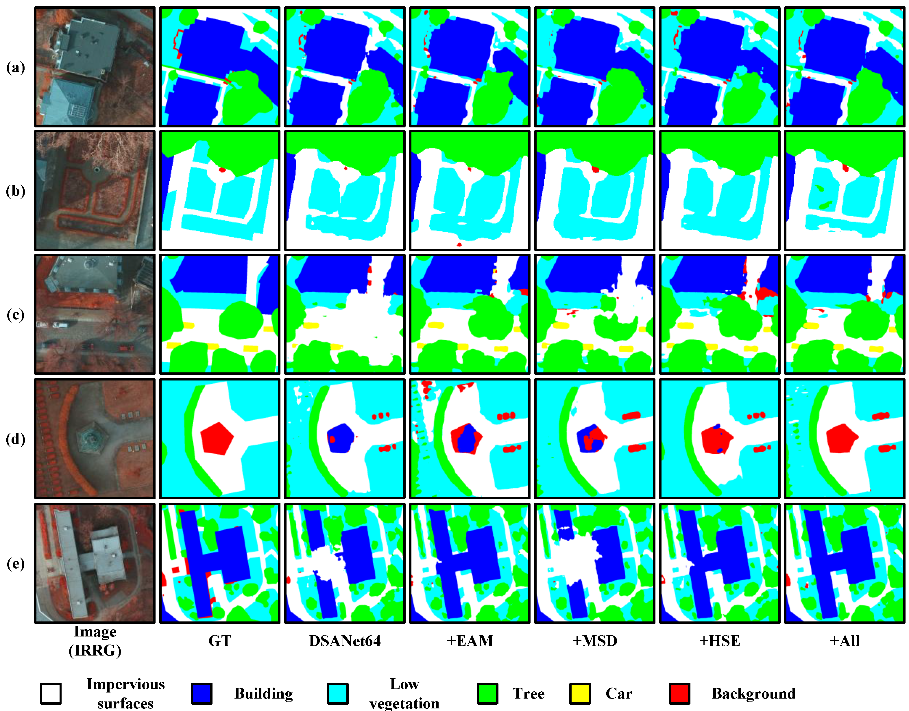
5.1.3. Effectiveness of DSANet

All the ablation experiments conducted based on the Potsdam dataset are shown in Table 7. Introducing the EAM can produce 1.12% and 0.70% gains in the mIoU and mF1 scores of the model, respectively. The MSD loss effectively improves the mIoU and mF1 scores by 0.91% and 0.58%, respectively. Introducing the HSE loss in the decoder can modestly enhance the mIoU by 0.28%. The MSD loss brings a 0.90% mIoU increase and a 0.57% mF1 increase. The EAM is the most effective module, as it is accompanied by model mIoU and mF1 growths of 1.12% and 0.71%, respectively. By comparing the backbone of DSANet64 with DSANet64 for 80,000 iterations and 320,000 iterations (see details in Figure 6), we find that the improvement yielded by DSANet is significant; even if the number of training iterations for the backbone network is increased to 4 times the original amount, it is still difficult to obtain better model performance, while DSANet64 is able to continue achieving improved model performance up to an mIoU of 80% with the increase in the number of training iterations.

5.2. Qualitative Analysis of Features

In order to examine the impact of various modules on the segmentation performance of the model, we visualize the obtained results in Figure 7. The visualization includes the original IRRG image, the labels, and the segmentation results of the backbone acquired after adding the feature enhancement modules separately and after adding all modules. Figure 7a–e are buildings, low-vegetation areas, trees, unmarked features, and buildings with complex boundaries, respectively. We observe that the results of segmentation based on the backbone frequently contain erroneous segmentation borders and even patch holes. Adding the EAM can effectively resolve the semantic discrimination issues, for example, by restoring the recognition results for the missing trees in Figure 7c. Adding MSD loss can help the segmentation process maintain better boundaries, but it cannot compensate for segmentation mistakes caused by semantics, such as identifying the connected buildings in Figure 7a while preserving the gaps in the buildings in Figure 7b,d. Adding the HSE loss can enhance the model’s capacity for semantic perception, preventing the occurrence of the problem of missing semantics. DSANet64 with EAM, MSD loss, and HSE loss can combine the capabilities of each module and complement their benefits, and its segmentation results are more accurate than those of the backbone network.

5.3. Quantitative Comparison with State-of-the-Art Methods

To measure the performance of our model, we compare DSANet with popular lightweight and efficient semantic segmentation networks whose numbers of parameters vary from 0.1 M to 21 M. We assess the performance of the models in terms of both accuracy and inference speed on both the Potsdam and Vaihingen datasets. To objectively evaluate the model performance, we fixed the cutoff threshold for the number of model parameters to 1.5 M.

Table 8. Comparison of DSANet with the State-of-the-Art Models on the Potsdam Dataset.

Method	Per-Class mIoU (%)					mIoU (%)	mF1 (%)	Params (M)
	Imperious Surface	Building	Low Vegetation	Tree	Car
FPENet [40]	76.55	86.30	65.56	66.48	67.16	72.41	83.64	0.11
FSSNet [37]	79.90	86.83	68.69	69.40	75.20	76.00	86.20	0.17
CGNet [67]	78.08	84.88	66.86	68.32	72.17	74.06	84.93	0.48
EDANet [35]	79.83	87.50	69.24	70.73	72.16	75.89	86.13	0.67
ContextNet [43]	79.37	86.86	68.70	69.38	71.96	75.25	85.71	0.86
LEDNet [41]	82.45	89.12	71.17	72.51	74.28	77.91	87.42	0.89
Fast-SCNN [37]	78.15	83.29	68.76	69.74	70.89	74.17	85.05	1.45
DSANet32	82.04	88.79	70.70	72.09	75.58	77.84	87.38	1.28
ESNet [68]	82.31	88.16	71.94	73.37	78.09	78.77	88.00	1.66
DABNet [34]	81.30	88.23	70.95	73.24	73.20	77.38	87.10	1.96
ERFNet [36]	80.38	88.18	70.81	72.30	74.89	77.31	87.06	2.08
DDRNet23-slim [48]	81.27	89.09	69.91	72.37	72.99	77.13	86.91	5.81
STDCNet [38]	82.07	89.41	71.45	73.49	76.78	78.64	87.90	8.57
LinkNet [39]	80.71	88.08	70.75	72.13	76.11	77.56	87.22	11.54
BiSeNetV1 [44]	81.91	88.95	71.83	73.21	80.18	79.22	88.27	13.42
BiSeNetV2 [45]	81.23	89.21	71.03	72.6	73.29	77.47	87.14	14.77
SFNet [47]	80.52	84.97	71.37	72.92	79.94	77.94	87.51	13.31
DDRNet23 [48]	82.58	90.07	71.56	73.55	75.44	78.64	87.89	20.59
DSANet64	83.02	89.50	71.86	74.26	77.34	79.20	88.25	4.65

reports the accuracy and inference speed results obtained on the Potsdam dataset.

5.3.1. Segmentation Performances Achieved on the Potsdam Dataset

The comparison between the results produced by DSANet and the other state-of-the-art models on the Potsdam dataset are shown in Table 8. Among the models with fewer than 1.5 M model parameters, DSANet32 obtains the best mIoU result of 75.58% on the car segmentation task and achieves suboptimal performance. In terms of the accuracy-speed tradeoff, DSANet32 achieves a balance between accuracy and inference speed. DSANet32 is over 2.2 times more accurate than LEDNet, the most accuracy network, and is 2.59% more accurate than ContextNet, the fastest network. Among the models with more than 1.5 M model parameters, DSANet64 works best to segment impervious surfaces and trees and achieves comparable results to those of BiSeNet V1, yielding 79.20 % mIoU and 88.25 % mF1 scores with 35 % of the number of parameters in BiSeNet V1. Figure 8 provides a more intuitive comparison of the segmentation results obtained by DSANet and the other models on the Potsdam dataset under the small size settings. Figure 9 shows the whole-image segmentation results of DSANet and the other models.

5.3.2. Segmentation Performances Achieved on the Vaihingen Dataset

The comparison between the results produced by DSANet and the other state-of-the-art models on the Vaihingen dataset are shown in

Table 9. Comparison of DSANet with the State-of-the-Art Models on the Vaihingen Dataset.

Method	Per-Class mIoU (%)					mIoU (%)	mF1 (%)
	Imperious Surface	Building	Low Vegetation	Tree	Car
FPENet [40]	78.37	84.24	63.44	73.79	44.39	68.85	80.67
FSSNet [37]	76.88	83.75	62.96	73.03	45.74	68.47	80.51
CGNet [67]	77.86	84.63	64.88	74.90	47.80	70.01	81.61
EDANet [35]	78.76	84.56	64.51	74.32	51.65	70.76	82.36
ContextNet [43]	77.77	83.65	61.99	73.15	50.32	69.38	81.31
LEDNet [41]	79.25	85.00	65.67	74.72	50.73	71.07	82.48
Fast-SCNN [37]	76.21	82.08	61.06	71.47	44.45	67.05	79.48
DSANet32	79.17	85.30	64.30	74.05	53.74	71.31	82.74
ESNet [68]	79.74	86.24	64.35	74.47	53.77	71.71	82.99
DABNet [34]	78.48	84.42	63.92	73.90	54.16	70.98	82.55
ERFNet [36]	79.34	85.68	64.07	74.51	54.01	71.52	82.88
DDRNet23-slim [48]	78.81	84.53	64.55	73.96	52.92	70.95	82.49
STDC1 [38]	79.03	85.76	64.27	73.69	48.71	70.29	81.84
LinkNet [39]	79.94	85.94	64.60	74.29	54.32	71.82	83.09
BiSeNetV1 [44]	78.84	85.55	64.23	74.15	50.50	70.65	82.17
BiSeNetV2 [45]	79.14	84.91	64.26	74.09	55.59	71.60	83.00
DSANet64	79.50	85.98	63.86	73.60	58.35	72.26	83.49

. Among the models with less than 1.5 M parameters, DSANet32 achieves the best results, with 85.30% and 53.74% mIoUs on the building and car segmentation tasks, respectively, and its overall 71.31% mIoU and 82.74% mF1 scores are impressive. In comparison with these other models, DSANet32 still obtains a better inference speed, although it has a disadvantage in terms of the number of required parameters. DSANet achieves the best car segmentation result, with an absolute 2.67% mIoU lead over the second-place method. DSANet64 achieves a 72.26% mIoU and a 83.49% mF1 on the Vaihingen dataset, which are also the best results. Figure 10 provides an intuitive comparison between the segmentation results obtained by DSANet and the other models on the Vaihingen dataset under the small size setting. Figure 11 shows the whole-image segmentation results of DSANet and the other models.

5.3.3. Inference Speeds

The comparison between the inference speed results produced by DSANet and the other state-of-the-art models under different image sizes are shown in

Table 10. FPS Results Obtained on the Potsdam Dataset Under Different Size Settings.

Method	mIoU (%)	FPS
		512	1024	6000
FPENet [40]	72.41	173.47	73.13	2.44
FSSNet [37]	76.00	527.26	183.30	6.27
CGNet [67]	74.06	127.51	66.78	0.58
EDANet [35]	75.89	390.17	135.50	4.37
ContextNet [43]	75.25	688.70	257.25	8.59
LEDNet [41]	77.91	293.48	104.92	3.74
Fast-SCNN [37]	74.17	670.82	261.43	8.60
DSANet32	77.84	648.49	245.66	8.78
ESNet [68]	78.77	295.33	100.27	2.77
DABNet [34]	77.38	173.47	73.13	2.44
ERFNet [36]	77.31	282.66	96.00	2.65
DDRNet23-slim [48]	77.13	429.09	208.38	6.98
STDC1 [38]	78.64	437.41	147.07	5.00
BiSeNetV1 [44]	79.22	351.89	128.64	3.92
BiSeNetV2 [45]	77.47	242.27	114.15	3.87
DDRNet23 [48]	78.64	256.65	99.58	3.46
DSANet64	79.20	470.07	172.16	5.46

. Our proposed DSANet32 reaches an inference speed of 8.78 on the 6000 × 6000 images, which are derived from the Potsdam dataset. In comparison with the fastest inference model at sizes of 512 and 1024, DSANet32 is only 6-7% behind ContextNet, whose segmentation performance is far behind that of DSANet32. In a comparison with the corresponding models, DSANet64 achieves the best inference speed at a size of 512 with 470.07 FPS. At the 1024 and 6000 sizes, DSANet64 still achieves comparable results. Figure 1 gives a visualization of the segmentation speed-accuracy tradeoffs provided by all models. The closer the model’s points are to the upper-right corner, the better that model performs in terms of the speed-accuracy tradeoff.

6. Conclusions

In this paper, we propose DSANet a deep supervision-based simple attention network, for large-scale RSI semantic segmentation; our network achieves an excellent balance between accuracy and inference speed. The main contributions of DSANet lie in three aspects: a simple attention module with linear complexity called the EAM, which is employed in the deepest network layer for long-range semantic information modeling; a improved deep supervision-based MSD loss for supervising portions of the feature map to directly learn the detailed spatial pyramid features; and a deep supervision-based HSE loss for supervising the network so that it learns the category frequency distribution of the training data.

Our DSANet provides consistently outstanding achievement on two benchmark datasets (i.e., the ISPRS Potsdam and Vaihingen datasets). On the ISPRS Potsdam test dataset, DSANet64 obtains a mean IoU of 79.20% at 5.46 FPS on 6000 × 6000 images and at 470.07 FPS on 512 × 512 images.

References

1. Liu, P. A survey of remote-sensing big data. Front. Environ. Sci. 2015, 3, 5. [Google Scholar] [CrossRef] [Green Version]
2. Laney, D. 3D data management: Controlling data volume, velocity and variety. META Group Res. Note 2001, 6, 1. [Google Scholar]
3. der Sande, C.V.; Jong, S.D.; Roo, A.D. A segmentation and classification approach of IKONOS-2 imagery for land cover mapping to assist flood risk and flood damage assessment. Int. J. Appl. Earth Obs. Geoinf. 2003, 4, 217–229. [Google Scholar] [CrossRef]
4. Costa, H.; Foody, G.M.; Boyd, D.S. Supervised methods of image segmentation accuracy assessment in land cover mapping. Remote Sens. Environ. 2018, 205, 338–351. [Google Scholar] [CrossRef] [Green Version]
5. Im, J.; Jensen, J.; Tullis, J. Object-based change detection using correlation image analysis and image segmentation. Int. J. Remote Sens. 2008, 29, 399–423. [Google Scholar] [CrossRef]
6. Chen, G.; Hay, G.J.; Carvalho, L.M.; Wulder, M.A. Object-based change detection. Int. J. Remote Sens. 2012, 33, 4434–4457. [Google Scholar] [CrossRef]
7. Du, S.; Du, S.; Liu, B.; Zhang, X. Mapping large-scale and fine-grained urban functional zones from VHR images using a multi-scale semantic segmentation network and object based approach. Remote Sens. Environ. 2021, 261, 112480. [Google Scholar] [CrossRef]
8. Wang, J.; Hu, X.; Meng, Q.; Zhang, L.; Wang, C.; Liu, X.; Zhao, M. Developing a method to extract building 3d information from GF-7 data. Remote Sens. 2021, 13, 4532. [Google Scholar] [CrossRef]
9. Li, P.; Guo, J.; Song, B.; Xiao, X. A multilevel hierarchical image segmentation method for urban impervious surface mapping using very high resolution imagery. IEEE J. Sel. Top. Appl. Earth Obs. Remote Sens. 2010, 4, 103–116. [Google Scholar] [CrossRef]
10. Miao, Z.; Fu, K.; Sun, H.; Sun, X.; Yan, M. Automatic water-body segmentation from high-resolution satellite images via deep networks. IEEE Geosci. Remote Sens. Lett. 2018, 15, 602–606. [Google Scholar] [CrossRef]
11. Long, J.; Shelhamer, E.; Darrell, T. Fully convolutional networks for semantic segmentation. In Proceedings of the IEEE Conference on Computer Vision and Pattern Recognition, Boston, MA, USA, 7–12 June 2015; pp. 3431–3440. [Google Scholar]
12. Ronneberger, O.; Fischer, P.; Brox, T. U-net: Convolutional networks for biomedical image segmentation. In Proceedings of the International Conference on Medical Image Computing and Computer-Assisted Intervention, Munich, Germany, 5–9 October 2015; pp. 234–241. [Google Scholar]
13. Zhang, Z.; Liu, Q.; Wang, Y. Road extraction by deep residual u-net. IEEE Geosci. Remote Sens. Lett. 2018, 15, 749–753. [Google Scholar] [CrossRef]
14. Heidler, K.; Mou, L.; Baumhoer, C.; Dietz, A.; Zhu, X.X. Hed-unet: Combined segmentation and edge detection for monitoring the antarctic coastline. IEEE Trans. Geosci. Remote Sens. 2021, 60, 1–14. [Google Scholar] [CrossRef]
15. Chen, L.-C.; Papandreou, G.; Schroff, F.; Adam, H. Rethinking atrous convolution for semantic image segmentation. arXiv 2017, arXiv:1706.05587. [Google Scholar]
16. Chen, L.-C.; Zhu, Y.; Papandreou, G.; Schroff, F.; Adam, H. Encoder-decoder with atrous separable convolution for semantic image segmentation. In Proceedings of the European Conference on Computer Vision (ECCV), Munich, Germany, 8–14 September 2018; pp. 801–818. [Google Scholar]
17. Yang, J.; Guo, J.; Yue, H.; Liu, Z.; Hu, H.; Li, K. CDnet: CNN-based cloud detection for remote sensing imagery. IEEE Trans. Geosci. Remote Sens. 2019, 57, 6195–6211. [Google Scholar] [CrossRef]
18. Liu, S.; Cheng, J.; Liang, L.; Bai, H.; Dang, W. Light-weight semantic segmentation network for UAV remote sensing images. IEEE J. Sel. Top. Appl. Earth Obs. Remote Sens. 2021, 14, 8287–8296. [Google Scholar] [CrossRef]
19. Lee, C.-Y.; Xie, S.; Gallagher, P.; Zhang, Z.; Tu, Z. Deeply-Supervised Nets. In Machine Learning Research, Proceedings of the Eighteenth International Conference on Artificial Intelligence and Statistics; Lebanon, G., Vishwanathan, S.V.N., Eds.; PMLR: San Diego, CA, USA, 2015; Volume 38, pp. 562–570. [Google Scholar]
20. Deng, C.; Liang, L.; Su, Y.; He, C.; Cheng, J. Semantic segmentation for high-resolution remote sensing images by light-weight network. In Proceedings of the 2021 IEEE International Geoscience and Remote Sensing Symposium IGARSS, Brussels, Belgium, 11–16 July 2021; pp. 3456–3459. [Google Scholar]
21. Liu, S.; Ding, W.; Liu, C.; Liu, Y.; Wang, Y.; Li, H. ERN: Edge loss reinforced semantic segmentation network for remote sensing images. Remote Sens. 2018, 10, 1339. [Google Scholar] [CrossRef] [Green Version]
22. Yuan, W.; Xu, W. Neighborloss: A loss function considering spatial correlation for semantic segmentation of remote sensing image. IEEE Access 2021, 9, 641–675. [Google Scholar] [CrossRef]
23. Simonyan, K.; Zisserman, A. Very deep convolutional networks for large-scale image recognition. arXiv 2014, arXiv:1409.1556. [Google Scholar]
24. He, K.; Zhang, X.; Ren, S.; Sun, J. Deep residual learning for image recognition. In Proceedings of the IEEE Conference on Computer Vision and Pattern Recognition, Las Vegas, NV, USA, 27–30 June 2016; pp. 770–778. [Google Scholar]
25. Huang, G.; Liu, Z.; Maaten, L.V.D.; Weinberger, K.Q. Densely connected convolutional networks. In Proceedings of the IEEE Conference on Computer Vision and Pattern Recognition, Honolulu, HI, USA, 21–26 July 2017; pp. 4700–4708. [Google Scholar]
26. Iandola, F.N.; Han, S.; Moskewicz, M.W.; Ashraf, K.; Dally, W.J.; Keutzer, K. SqueezeNet: AlexNet-level accuracy with 50x fewer parameters and <0.5 MB model size. arXiv 2016, arXiv:1602.07360. [Google Scholar]
27. Krizhevsky, A.; Sutskever, I.; Hinton, G.E. Imagenet classification with deep convolutional neural networks. In Proceedings of the Advances in Neural Information Processing Systems, Lake Tahoe, NV, USA, 3–8 December 2012; pp. 1097–1105. [Google Scholar]
28. Howard, A.G.; Zhu, M.; Chen, B.; Kalenichenko, D.; Wang, W.; Weyand, T.; Andreetto, M.; Adam, H. Mobilenets: Efficient convolutional neural networks for mobile vision applications. arXiv 2017, arXiv:1704.04861. [Google Scholar]
29. Sandler, M.; Howard, A.; Zhu, M.; Zhmoginov, A.; Chen, L.-C. Mobilenetv2: Inverted residuals and linear bottlenecks. In Proceedings of the IEEE Conference on Computer Vision and Pattern Recognition, Salt Lake City, UT, USA, 18–22 June 2018; pp. 4510–4520. [Google Scholar]
30. Howard, A.; Sandler, M.; Chu, G.; Chen, L.-C.; Chen, B.; Tan, M.; Wang, W.; Zhu, Y.; Pang, R.; Vasudevan, V.; et al. Searching for mobilenetv3. In Proceedings of the IEEE/CVF International Conference on Computer Vision, Long Beach, CA, USA, 16–20 June 2019; pp. 1314–1324. [Google Scholar]
31. Zhang, X.; Zhou, X.; Lin, M.; Sun, J. Shufflenet: An extremely efficient convolutional neural network for mobile devices. In Proceedings of the IEEE Conference on Computer Vision and Pattern Recognition, Salt Lake City, UT, USA, 18–22 June 2018; pp. 6848–6856. [Google Scholar]
32. Ma, N.; Zhang, X.; Zheng, H.-T.; Sun, J. Shufflenet v2: Practical guidelines for efficient CNN architecture design. In Proceedings of the European Conference on Computer Vision (ECCV), Munich, Germany, 14–18 September 2018; pp. 116–131. [Google Scholar]
33. Paszke, A.; Chaurasia, A.; Kim, S.; Culurciello, E. Enet: A deep neural network architecture for real-time semantic segmentation. arXiv 2016, arXiv:1606.02147. [Google Scholar]
34. Li, G.; Yun, I.; Kim, J.; Kim, J. Dabnet: Depth-wise asymmetric bottleneck for real-time semantic segmentation. In Proceedings of the British Machine Vision Conference (BMVC), Cardiff, UK, 9–12 September 2019; pp. 186.1–186.12. [Google Scholar]
35. Lo, S.-Y.; Hang, H.-M.; Chan, S.-W.; Lin, J.-J. Efficient dense modules of asymmetric convolution for real-time semantic segmentation. In Proceedings of the ACM Multimedia Asia, Nice, France, 21–25 October 2019; pp. 1–6. [Google Scholar]
36. Romera, E.; Alvarez, J.M.; Bergasa, L.M.; Arroyo, R. Erfnet: Efficient residual factorized convnet for real-time semantic segmentation. IEEE Trans. Intell. Transp. Syst. 2017, 19, 263–272. [Google Scholar] [CrossRef]
37. Zhang, X.; Chen, Z.; Wu, Q.J.; Cai, L.; Lu, D.; Li, X. Fast semantic segmentation for scene perception. IEEE Trans. Industr. Inform. 2018, 15, 1183–1192. [Google Scholar] [CrossRef]
38. Fan, M.; Lai, S.; Huang, J.; Wei, X.; Chai, Z.; Luo, J.; Wei, X. Rethinking bisenet for real-time semantic segmentation. In Proceedings of the IEEE/CVF Conference on Computer Vision and Pattern Recognition, Montreal, QC, Canada, 11–17 October 2021; pp. 9716–9725. [Google Scholar]
39. Chaurasia, A.; Culurciello, E. Linknet: Exploiting encoder representations for efficient semantic segmentation. In Proceedings of the 2017 IEEE Visual Communications and Image Processing (VCIP), Venice, Italy, 22–29 October 2017; pp. 1–4. [Google Scholar]
40. Liu, M.; Yin, H. Feature pyramid encoding network for real-time semantic segmentation. arXiv 2019, arXiv:1909.08599. [Google Scholar]
41. Wang, Y.; Zhou, Q.; Liu, J.; Xiong, J.; Gao, G.; Wu, X.; Latecki, L.J. Lednet: A lightweight encoder-decoder network for real-time semantic segmentation. In Proceedings of the 2019 IEEE International Conference on Image Processing (ICIP), Taipei, Taiwan, 22—25 September 2019; pp. 1860–1864. [Google Scholar]
42. Poudel, R.P.; Liwicki, S.; Cipolla, R. Fast-scnn: Fast semantic segmentation network. arXiv 2019, arXiv:1902.04502. [Google Scholar]
43. Poudel, R.P.; Bonde, U.; Liwicki, S.; Zach, C. Contextnet: Exploring context and detail for semantic segmentation in real-time. arXiv 2018, arXiv:1805.04554. [Google Scholar]
44. Yu, C.; Wang, J.; Peng, C.; Gao, C.; Yu, G.; Sang, N. Bisenet: Bilateral segmentation network for real-time semantic segmentation. In Proceedings of the European Conference on Computer Vision (ECCV), Munich, Germany, 8–14 September 2018; pp. 325–341. [Google Scholar]
45. Yu, C.; Gao, C.; Wang, J.; Yu, G.; Shen, C.; Sang, N. Bisenet v2: Bilateral network with guided aggregation for real-time semantic segmentation. Int. J. Comput. Vis. 2021, 129, 3051–3068. [Google Scholar] [CrossRef]
46. Li, H.; Xiong, P.; Fan, H.; Sun, J. Dfanet: Deep feature aggregation for real-time semantic segmentation. In Proceedings of the IEEE/CVF Conference on Computer Vision and Pattern Recognition, Long Beach, CA, USA, 15–20 June 2019; pp. 9522–9531. [Google Scholar]
47. Li, X.; You, A.; Zhu, Z.; Zhao, H.; Yang, M.; Yang, K.; Tan, S.; Tong, Y. Semantic flow for fast and accurate scene parsing. In European Conference on Computer Vision; Springer: Berlin/Heidelberg, Germany, 2020; pp. 775–793. [Google Scholar]
48. Hong, Y.; Pan, H.; Sun, W.; Jia, Y. Deep dual-resolution networks for real-time and accurate semantic segmentation of road scenes. arXiv 2021, arXiv:2101.06085. [Google Scholar]
49. Zhao, H.; Shi, J.; Qi, X.; Wang, X.; Jia, J. Pyramid scene parsing network. In Proceedings of the IEEE Conference on Computer Vision and Pattern Recognition, Honolulu, HI, USA, 21–26 July 2017; pp. 2881–2890. [Google Scholar]
50. Chen, L.-C.; Papandreou, G.; Kokkinos, I.; Murphy, K.; Yuille, A.L. Semantic image segmentation with deep convolutional nets and fully connected crfs. arXiv 2014, arXiv:1412.7062. [Google Scholar]
51. Chen, L.C.; Papreou, G.; Kokkinos, I.; Murphy, K.; Yuille, A.L. Deeplab: Semantic image segmentation with deep convolutional nets, atrous convolution, and fully connected crfs. IEEE Trans. Pattern Anal. Mach. Intell. 2017, 40, 834–848. [Google Scholar] [CrossRef] [Green Version]
52. Fu, J.; Liu, J.; Tian, H.; Li, Y.; Bao, Y.; Fang, Z.; Lu, H. Dual attention network for scene segmentation. In Proceedings of the IEEE/CVF Conference on Computer Vision and Pattern Recognition, Long Beach, CA, USA, 15–20 June 2019; pp. 3146–3154. [Google Scholar]
53. Yuan, Y.; Chen, X.; Wang, J. Object-contextual representations for semantic segmentation. In European Conference on Computer Vision; Springer: Berlin/Heidelberg, Germany, 2020; pp. 173–190. [Google Scholar]
54. Hu, J.; Shen, L.; Sun, G. Squeeze-and-excitation networks. In Proceedings of the IEEE Conference on Computer Vision and Pattern Recognition, Salt Lake City, UT, USA, 18–22 June 2018; pp. 7132–7141. [Google Scholar]
55. Park, J.; Woo, S.; Lee, J.-Y.; Kweon, I.S. Bam: Bottleneck attention module. arXiv 2018, arXiv:1807.06514. [Google Scholar]
56. Woo, S.; Park, J.; Lee, J.-Y.; Kweon, I.S. Cbam: Convolutional block attention module. In Proceedings of the European Conference on Computer Vision (ECCV), Munich, Germany, 8–14 September 2018; pp. 3–19. [Google Scholar]
57. Meng, Q.; Zhao, M.; Zhang, L.; Shi, W.; Su, C.; Bruzzone, L. Multilayer feature fusion network with spatial attention and gated mechanism for remote sensing scene classification. IEEE Geosci. Remote Sens. Lett. 2022, 19, 1–5. [Google Scholar] [CrossRef]
58. Ambartsoumian, A.; Popowich, F. Self-attention: A better building block for sentiment analysis neural network classifiers. arXiv 2018, arXiv:1812.07860. [Google Scholar]
59. Vaswani, A.; Shazeer, N.; Parmar, N.; Uszkoreit, J.; Jones, L.; Gomez, A.N.; Kaiser, L.; Polosukhin, I. Attention is all you need. In Proceedings of the Advances in Neural Information Processing Systems, Long Bench, CA, USA, 4–9 December 2017; pp. 5998–6008. [Google Scholar]
60. Dosovitskiy, A.; Beyer, L.; Kolesnikov, A.; Weissenborn, D.; Zhai, X.; Unterthiner, T.; Dehghani, M.; Minderer, M.; Heigold, G.; Gelly, S.; et al. An image is worth 16 × 16 words: Transformers for image recognition at scale. arXiv 2020, arXiv:2010.11929. [Google Scholar]
61. Liu, Z.; Lin, Y.; Cao, Y.; Hu, H.; Wei, Y.; Zhang, Z.; Lin, S.; Guo, B. Swin transformer: Hierarchical vision transformer using shifted windows. In Proceedings of the IEEE/CVF International Conference on Computer Vision, Montreal, QC, Canada, 10–17 October 2021; pp. 10012–10022. [Google Scholar]
62. Wang, W.; Xie, E.; Li, X.; Fan, D.-P.; Song, K.; Liang, D.; Lu, T.; Luo, P.; Shao, L. Pyramid vision transformer: A versatile backbone for dense prediction without convolutions. In Proceedings of the IEEE/CVF International Conference on Computer Vision, Montreal, QC, Canada, 11–17 October 2021; pp. 568–578. [Google Scholar]
63. Li, R.; Zheng, S.; Zhang, C.; Duan, C.; Wang, L.; Atkinson, P.M. Abcnet: Attentive bilateral contextual network for efficient semantic segmentation of fine-resolution remotely sensed imagery. ISPRS J. Photogramm. Remote Sens. 2021, 181, 84–98. [Google Scholar] [CrossRef]
64. Wang, S.; Li, B.Z.; Khabsa, M.; Fang, H.; Ma, H. Linformer: Self-attention with linear complexity. arXiv 2020, arXiv:2006.04768. [Google Scholar]
65. Guo, M.-H.; Liu, Z.-N.; Mu, T.-J.; Hu, S.-M. Beyond self-attention: External attention using two linear layers for visual tasks. arXiv 2021, arXiv:2105.02358. [Google Scholar] [CrossRef]
66. Maggiori, E.; Tarabalka, Y.; Charpiat, G.; Alliez, P. Convolutional Neural Networks for Large-Scale Remote-Sensing Image Classification. IEEE Trans. Geosci. Remote Sens. 2017, 55, 645–657. [Google Scholar] [CrossRef] [Green Version]
67. Wu, T.; Tang, S.; Zhang, R.; Cao, J.; Zhang, Y. Cgnet: A light-weight context guided network for semantic segmentation. IEEE Trans. Image Process. 2020, 30, 1169–1179. [Google Scholar] [CrossRef]
68. Wang, Y.; Zhou, Q.; Xiong, J.; Wu, X.; Jin, X. Esnet: An efficient symmetric network for real-time semantic segmentation. In Chinese Conference on Pattern Recognition and Computer Vision (PRCV); Springer: Berlin/Heidelberg, Germany, 2019; pp. 41–52. [Google Scholar]
Figure 1. Speed-accuracy tradeoff yielded by different semantic segmentation methods on the ISPRS Potsdam dataset with a size of 6000 × 6000 pixels using an RTX 3090 GPU. Orange points: different versions of our proposed method. Red points: lightweight methods with more than 1.5 M parameters. Blue points: lightweight methods with less than 1.5 M parameters. Our proposed methods achieve the best speed-accuracy tradeoffs. It is worth noting that that the sizes of the corresponding points of the methods are positively correlated with their parameters.
Remotesensing 14 05399 g001
Figure 2. The network architecture of DSANet. Note that the green blocks are encoder components, whereas the red blocks and the semantic segmentation head are decoder components. All auxiliary segmentation heads within the dashed box are only engaged during model training, whereas only the remaining modules use inference time.
Remotesensing 14 05399 g002
Figure 3. Dot product self-attention SA (A) and two kinds of embedding self-attention: EAM I (B) and EAM II (C).
Remotesensing 14 05399 g003
Figure 4. Schematic diagram of the MSD loss calculation process. Stridds 1, 2, and 4 in the Laplace convolution operator are denoted as S1, S2 and S4.
Remotesensing 14 05399 g004
Figure 5. Schematic diagram of the HSE vector calculation process with 4 levels. (a) Boundaries in different colors indicate different segmentation scales. (b) Simplified diagram of the local frequency distribution. (c) Visual presentation of the HSE vectors.
Remotesensing 14 05399 g005
Figure 6. Comparisons between the mean IoU results of the DSANet64 backbone and DSANet64 with 80,000 iterations and 320,000 iterations on the Potsdam dataset.
Remotesensing 14 05399 g006
Figure 7. Comparison between the segmentation results of the DSANet64 backbone and the EAM, MSD, and HSE modules. (ae) are derived from the Potsdam dataset. GT denotes the ground truth.
Remotesensing 14 05399 g007
Figure 8. Examples of segmentation results derived from the Potsdam dataset under the small size setting. (a) IRRG image. (b) Ground truth. (c) FPENet. (d) FSSNet. (e) CGNet. (f) ContextNet. (g) Fast-SCNN. (h) ERFNet. (i) STDC1. (j) LinkNet. (k) ICNet34. (l) BiSeNet V1. (m) SFNet. (n) DDRNet23. (o) DSANet64.
Remotesensing 14 05399 g008
Figure 9. Examples of segmentation results derived from the Potsdam dataset with the whole image size setting. (a) IRRG image. (b) Ground truth. (c) FPENet. (d) ERFNet. (f) STDC1. (g) BiSeNet V1. (h) BiSeNet V2. (i) DSANet64.
Remotesensing 14 05399 g009
Figure 10. Examples of segmentation results derived from the Vaihingen dataset under the small size setting. (a) IRRG image. (b) Ground truth. (c) FPENet. (d) FSSNet. (e) CGNet. (f) ContextNet. (g) Fast-SCNN. (h) ESNet. (i) ERFNet. (j) DDRNet23-slim. (k) STDC1. (l) LinkNet. (m) BiSeNet V1. (n) BiSeNet V2. (o) DSANet64.
Remotesensing 14 05399 g010
Figure 11. Examples of segmentation results derived from the Vaihingen dataset with the whole image size setting. (a) IRRG image. (b) Ground truth. (c) FPENet. (d) ERFNet. (e) DDRNet23-slim. (f) STDC1. (g) BiSeNet V1. (h) BiSeNet V2. (i) DSANet64.
Remotesensing 14 05399 g011