Impact of Multi-Thresholds and Vector Correction for Tracking Precipitating Systems over the Amazon Basin

Abstract

Different algorithms for forecasting and tracking meteorological systems have been developed over the years. Many of them are used to study cloud propagation, precipitation and lightning for nowcasting. Therefore, it is necessary to define carefully the parameters (e.g., intensity thresholds and minimum size) that impact tracking of these variables. In order to represent the physical aspects of rain propagation over the Amazon region, several methods of correction and displacement detection were studied. Different parameters were used to validate the methods based on the extrapolated rain cell. A probability detection of 78.4% and 68.6% was achieved for 20 dBZ thresholds during the wet and dry season, respectively. However, the POD decreases for higher reflectivity thresholds. The results for corrections by Inner Nuclei showed that embedded convection can dictate the propagation of rain cells. Split and merge corrections performed well; however, they applied only to a few cases. Corrections performed better for precipitating systems with larger areas and longer duration. The correction methods showed similar skills for both seasons. Which shows that they are able to monitor rain cells throughout the year. The automated combination of different methods for the 20 dBZ threshold proved to be the best choice for tracking rainfall in the Amazon region.

1. Introduction

The atmospheric systems occurring in the Amazon are strongly connected with the regulation of regional and global climate [1]. The seasonality of rainfall in the Amazon region is modulated in two periods, dry and wet [2]. In particular, convective systems are responsible for producing a large proportion of the intense precipitation throughout the Amazon region [3,4]. In the dry seasons, these systems can propagate over large extensions, including the central part of the Amazon Basin [5]. The dynamic and thermodynamic structures of these systems [6] can support the formation of isolated or multi-cellular thunderstorms. Some of those systems are composed of cloud towers of cumulonimbus embedded within a region with more stratiform clouds [7]. Therefore, tracking these rainfall systems is of paramount importance to measuring their impacts both globally and locally. However, to ensure that an unsupervised tool is capable of reliable results, it is necessary to deeply analyze the impacts of the parameters that define a realistic tracking, which is the main objective of this study.

During the wet season, Precipitating Systems (PSs) generally have large size rain cells with relatively low reflectivity and a longer life cycle. In contrast, during the dry season, PSs have greater intensity and smaller sizes [8]. These characteristics must be considered for short-term forecasting systems because the regional properties of weather events are crucial for a better prediction [9].

To study PSs, satellite images and meteorological radar are the most used instruments. The information representing the physical structures of precipitation cells can be used as a target to track their evolution and displacement [10]. Algorithms like ForTraCC (Forecast and Tracking the Evolution of Cloud Clusters) [11] and TITAN (Thunderstorm Identification, Tracking, Analysis, and Nowcasting) [12] utilize techniques based on the boundary thresholds of rain cells to track their displacement and life cycle. In recent years, several algorithms based on techniques such as contour thresholds, centroid, spatial cross-correlation, etc., have been developed and used to identify, track, and forecast very short-term (i.e., nowcasting) large-intensity precipitation events [13]. In a similar way to the aforementioned algorithms, the tool created for this study also uses thresholding and tracking via overlapping object areas.

The rain cells (targets) are usually non-rigid objects, i.e., they can eventually change shape in a given observation [14]. Moreover, they may experience multiple merging and splitting [15] during their lifespan. For techniques that rely on object shape to define tracking and prediction, such changes can affect the quality of this information. Since there is no simple unified solution, different approaches [16,17,18,19,20,21] can be applied to solve this problem. Understanding the regional characteristics of rainfall events can help to mitigate uncertainties related to tracking and forecasting.

In [8], it was found that during the dry season the thermodynamic environment favors the formation of isolated convective systems with more intense precipitation rates. In [22], it was observed that more organized convective systems (such as squall lines) are more frequent in the wet than in the dry season. In this study, it is believed that the frequency of occurrence of the different precipitating systems is affected by the different environmental characteristics of each season. Therefore, investigating the characteristics of PSs during distinct periods and identifying the best parameters to use as tracking metrics for algorithms can help characterize the phenomena around their development over the region [23]. Furthermore, this approach is a contribution to understanding the events with more complex dynamics in the Amazon Basin.

The main objective of this study is to investigate the impacts of different thresholds and different displacement vector correction methods on the tracking of precipitating systems. As there is no reference about the tracking, the validation was carried out by comparing the prediction of the rain cells, extrapolated as a function of the threshold and corrected vector, and the respective observation. More details will be shown in Section 2.3. Moreover, analyses were carried out to characterize the impact of physical differences observed between PSs in two seasons (e.g., dry and wet). First, different methods are applied to handle interaction classes such as mergers and splits of rain cells throughout the life cycle of PSs. Then, the method that best fits regional characteristics is used to analyze the patterns of the tracked systems and morphological features that most impact the tracking of PSs over the Amazon region. The results presented in this paper are part of a method that will be made available by INPE (the National Institute for Space Research) and its partners. This tool can be used for analysis across different regions and with multiple sensors.

The following section describes how the algorithm works and how the displacement correction methods were implemented. In particular, a detailed description is given for the validation of the correction methods by extrapolation. Section 3 presents the results of applying this algorithm to the two intensive operational periods (IOPs) of the GoAmazon experiment. We focus on investigating the characteristics of the tracked systems and their impacts on the performance of the tracking method. Conclusions and future perspectives are given in Section 3.

2. Data and Methodology

2.1. Data

Volumetric observations from the SIPAM S-band radar (Amazon Protection System), located in Manaus (Figure 1), were used, as in [24]. The dataset is based on measurements carried out during 2014 and 2015 in the GoAmazon (Green Ocean Amazon) experiment [25]. For this study, the Intense Observation Period (IOP) data were selected to analyze the characteristics of PS at different times during the year 2014. The IOPs were divided into two periods of observation. The first of these, IOP1, corresponds to observations between 1 February and 31 March 2014 (59 days). The second period (IOP2) corresponds to observations from 15 August to 15 October (61 days). The CAPPI (Constant Altitude Plane Position Indicator) product was used, based on the volumetric observations of the S-band radar of the SIPAM (Amazon Protection System), located in Manaus (Figure 1). The CAPPI product has a temporal resolution of 12 min, 40 altitude levels with 500 m each and a horizontal resolution of 2 × 2 km (range of 480 km). The radar reflectivity (dBZ) data from the 2.5 km level were used.

2.2. The Algorithm

Different approaches can be used [10,11,12,18,19,20,26,27,28] for object tracking, especially when the targets are non-rigid objects such as rain cells. Therefore, different techniques can be used for the same purpose. Here, a method based on geometry overlapping techniques to extract displacement vectors from the centroids of rain cells is applied. The algorithm aims to identify, track, and forecast individual cells of precipitation from weather radar data. This new algorithm considers the interaction of rain cells during their development and propagation. Some initial physical parameters need to be established to track the rainy systems over the Amazon region, such as minimum size and identification threshold. This has a direct impact on the definition of some morphological characteristics of the precipitating systems, such as the average size of the systems and the internal nuclei of each rain cell, which also affect their average lifetime. However, there are a number of processes that need to be carried out for the tracking to be effectively built. Further details on each one are given below.

Figure 2 shows the workflow of the algorithm. The processing stages have been divided into four parts: identification, tracking, corrections, and forecast. The identification step involves operations to identify rainy clusters (i.e., rain cells) and transform them into vectorial objects (polygons). Then, in the tracking step, geometries of two consecutive times are compared to extract the displacement information of the rain cell. However, corrections may be required in the tracking step associated with unrealistic displacement vectors. These errors occur due to sudden changes in the shape of the rain cells between two consecutive radar images, which may be associated with cell fusions and split, and failures in radar measurements, among other things. The last part refers to the validation of the correction method for each rain cell (reflectivity cluster based on the CAPPI product). For this, we use the rain cell forecast for the next time ahead, based on the corrected displacement vector, compared to the observed rain cell. It is verified which correction method and which tracking parameters performed better for each rain cell at each time step. This type of validation can be called conservative or persistent [28,29], considering that the changes in the next observation time will be small. 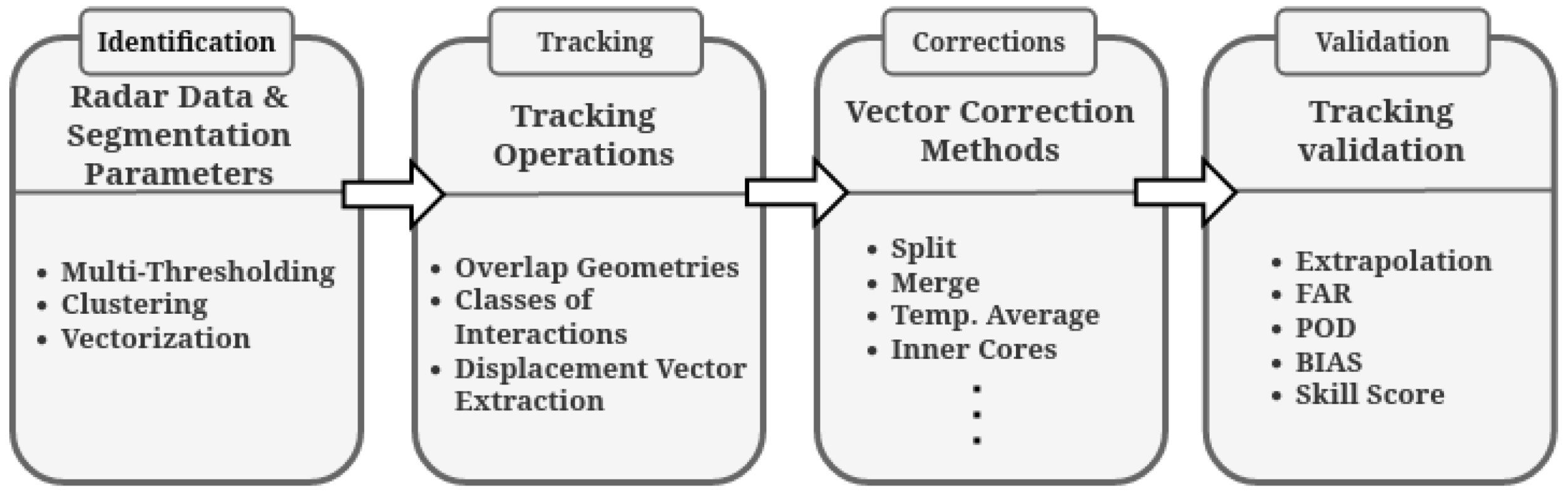The next sections describe in more detail some modules of the algorithm.

2.2.1. Identification Scope

The first scope of the algorithm aims to identify the morphological characteristics (i.e., shape, size, inner clusters, etc) of the rain cells. This is performed through segmentation of the radar images, where a filtering process (thresholding) is applied to highlight regions of interest. This is a typical process also known as image segmentation [30].

The clusters were selected based on the contour thresholds of the rain cells. In many studies [4,8,31,32], morphological characteristics of precipitating systems are described over the Amazon. In these studies, rain cells were observed that have radar reflectivity thresholds from 20 (both stratiform and convective precipitation are included) to 35 dBZ (more convective precipitation). Given this range, we selected the parameters of multi-thresholds that represented the boundary regions of the rain cells and used these parameters as follows: identification thresholds: 20, 30, and 35 dBZ; first inner thresholds: 30, 35, and 40 dBZ; second inner thresholds: 35, 40 and 45 dBZ.

Continuing with identification, the clustering method objective is to categorize groups of segmented points after the thresholding process. During this process, the rain cells are identified and labeled based on the clustering of pixels equal or larger than the predefined threshold. The label is an identification number of the rain cell for the current observation time. To perform this procedure, a well-known technique in machine learning was chosen. The DBSCAN (Density-Based Spatial Clustering of Applications with Noise) algorithm was applied to identify the clusters [33] or rain cells. It operates based on a distance between points in the neighborhood. A distance radius represents a proximity relation between neighbors and is defined by parameter Eps (Epsilon is a radius distance for neighborhood points), which corresponds to a minimum distance between points in the neighborhood. Another parameter of DBSCAN is a minimum number of neighbors, given by the minimum points, which is the least amount of nearby elements between points around one cluster [33].

Finally, the vectorization method is responsible for transforming clusterized points (rain pixels) that are in matrix format into vector-based. That information corresponds to the outer limits of each cell. Based on this conversion, it is possible to perform spatial operations between geometries of each cell at consecutive times, for instance: overlap, intersect, within, etc. This makes the process of analyzing overlaps between consecutive images even more manageable, because parameters such as the overlapping area of rainy events are easily adjustable.

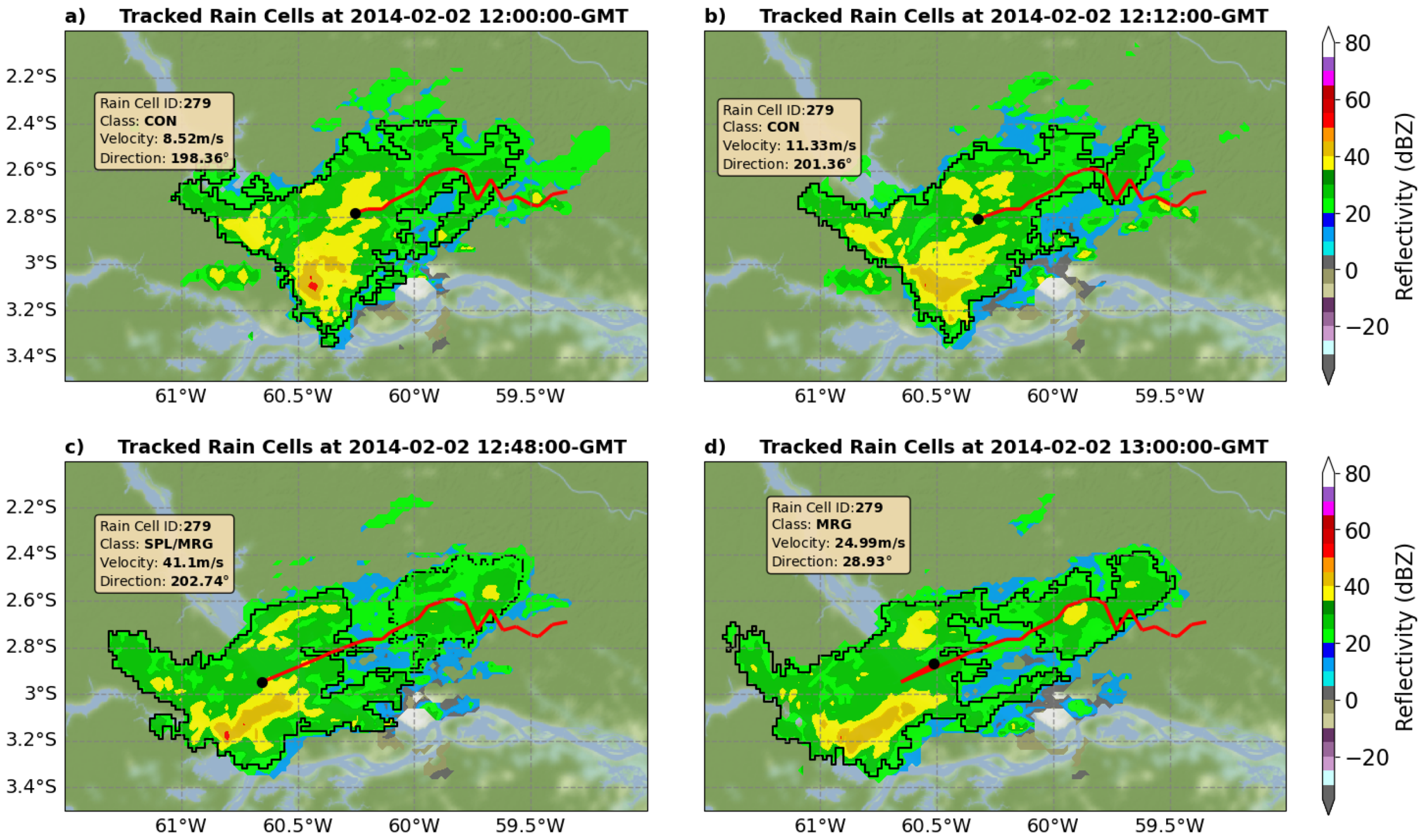
2.2.2. Tracking

The tracking module uses information from two consecutive times and extracts the trajectory of the PSs. The technique used to investigate the movement of rain cells and obtain their displacement vector takes into account the centroid of these clusters with a certain area of overlap at consecutive times. Overlapping cell geometries provide this association at subsequent times. Using this overlap criteria, it is possible to classify the event according to its classes (e.g., continuous, splits, and mergers) for the current observation time (t). Such a process is well known and applied by several algorithms [11,12,34]. However, depending on the applied technique for defining the geometry of rain cells, centroid positioning can suffer variations that directly impact the computation of the velocity and position of targets along the trajectory. To reduce these problems, the definitions applied in the previous section tend to smooth the shapes of tracked objects because they can disregard “gaps” at the edges and holes due to pixel-to-pixel thresholding, typical of tracking algorithms such as ForTraCC.

Each individual cell has information such as size, expansion rate, average reflectivity, centroid coordinates, velocity, direction, etc. This information defines the association between rain cells at consecutive times and establishes the trajectory. Here, the similarity criterion adopted considers the rain cells with a minimum percentage of overlap, which in this case was defined as 10%. Based on this definition we extracted the displacement vector $\overrightarrow{V}$ which goes from the centroid of a cell in time ($t-1$) to the centroid of the cell in the current time (t); this method was based on the algorithm ForTraCC [11].

As described by [11] for cloud clusters, multiple merging and splitting of rain cells can occur during their life cycle. Such behavior may be related to the interaction of systems, in different stages of their lifespan, along their trajectories, and even to multi-cell systems [7]. In order to describe the situations that can occur during the development of PSs, we characterize the transition events between two consecutive times with the interaction classes:

• New Rain Cell (NEW): While comparing two successive times, there is no overlap of areas between cell geometries at times $t-1$ and t. In this situation, it is considered that there was a spontaneous generation of a new system and a new life cycle is started from a cell at time t;
• Continuous (CON): While comparing two successive times $t-1$ and t, there is a unique overlap between geometries of the two cells;
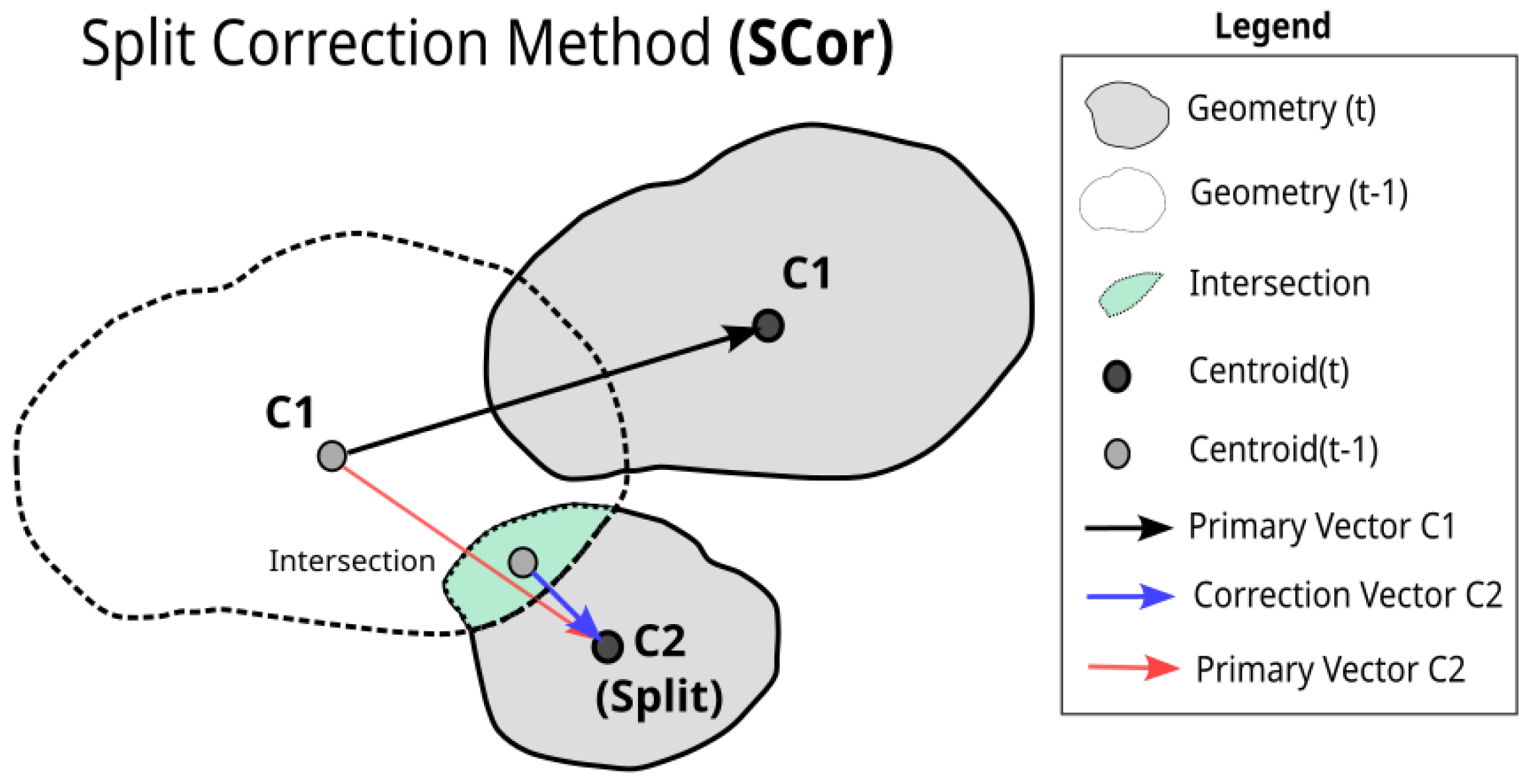
• Split (SPL): This situation occurs when two or more cells at time t overlap with the geometry of a cell at time $t-1$. In this case, a cell with the largest area at time t is classified as SPL, and a displacement vector starting from the centroid of cell $t-1$ is added to the track. The cell with the smallest area at time $t-1$ has its life cycle terminated or proceeds as a new system at the next time;
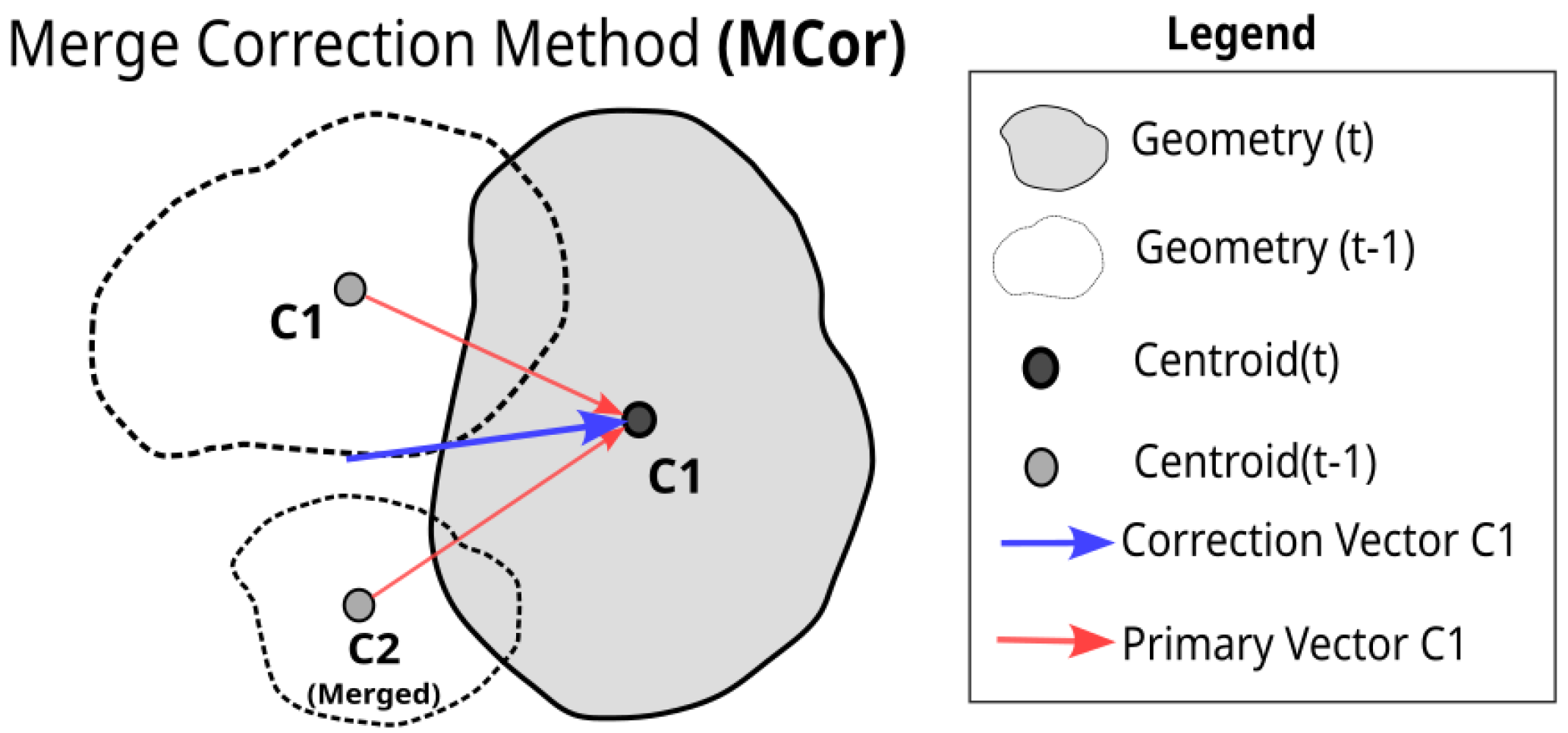
• Merge (MRG): The opposite situation to splitting (SPL), where two cells at time $t-1$ overlap into just a single cell at time t. In this case, the rain cell at time t receives the same relational entities as the cell with a larger area at time $t-1$, while the other cell ends its life cycle.

2.2.3. Correction Scope

Several factors can modify rain cell movement when analyzing their trajectory. One of these factors that can affect a reasonable estimate of displacement trajectory is the use of a centroid as a target. This problem is associated with the shape of tracked objects and processes of mergers and splits that may occur during the development of precipitating systems. According to [15], this problem comes from an object tracking perspective with multiple merging and splitting events for non-rigid objects.

In order to illustrate this problem, Figure 3 shows the tracking of a precipitating system over Manaus city on 2 February 2014. It is seen that during the transition between Figure 3a and Figure 3b the rain cell with ID 279 is classified as continuous (CON), and by applying displacement vector extraction based on the centroid of geometries, velocities of 8.52 and 11.33 m/s in the directions $198.{36}^{\circ }$ and $201.{36}^{\circ }$ were obtained, respectively. However, in Figure 3c,d, it is possible to note that a split and a merge occur on rain cell 279. The velocity and direction of the rain cell are unrealistic because of the sudden change in the shape. The red lines serve only to illustrate the trajectories of the centroids at previous times to the observed ones.

Mitigating this problem is the main objective of this study, and details about the proposed methods to reduce the uncertainties concerning the calculation of the displacement vector are given below.

Correction for Rain Cell Split

As will be seen in Section 3, rain cell split can occur with a frequency larger than 10%. The proposed vector correction method adds a new vector for a newly generated cell. This displacement vector starts from the centroid of the intersecting area between the rain cell at $t-1$ and a cell at time t generated after a Split, instead of from the centroid related to the rain cell in t. Figure 4 shows the visualization scheme for how the Split Correction method (SCor) works. It is believed that this type of correction will have the most significant impact on storm events that have deep convective cores with different directions, common in supercells [7]. Moreover, fragmentation of rain cells are frequent in the dissipation stages and may take advantage of this type of correction [35]. So this method solves a specific case: new smaller cells that arise from a split.

Correction for Rain Cell Merge

Throughout a precipitating system’s life cycle, it is common for it to merge with nearby cells. This may occur by several factors, larger systems propagating by absorbing new systems ahead [36], faster systems that join with slower systems, etc. Moreover, depending on the threshold applied for tracking, cell joining can also occur in multicell systems, where nearby convective cores with different stages of maturation can be merged [7]. Considering this feature, the Merge Correction Method (MCor) is applied to correct displacement in rain cell merge. The method uses a simple approach, where a set of vectors between current observation time (t) and vectors from the previous time ($t-1$) can define a correction for current displacement vector ${\overrightarrow{V}}_t$. In Figure 5, we visualize how the MCor method carries out correction by replacing a vector during an event of cell–cell merging. The filled gray polygon represents the cell at current time t and its corresponding vector before the correction (red arrow), the polygon at the previous time ($t-1$) is represented without the fill (transparent polygon). For rain cell merge, the interaction vectors between cells that precede the merge are considered, meaning that in Figure 5, the red arrow represents the primary vector coming from the interaction between geometries at t and $t-1$ and, the blue arrow is the correction vector made by MCor. The blue vector is the average of these red vectors (Equation (1)).

$${\overrightarrow{V}}_{avg}=\frac{1}{n}\sum _{i=1}^n{\overrightarrow{V}}_i$$

(1)

Temporal Average Correction Based on the Life Cycle of Precipitating Systems

The displacement vector often suffers abrupt changes in the values of velocity and direction caused by many circumstances, such as data gaps, sudden changes in the shape of rain cell polygons, holes in the polygons, and/or merging/splitting of systems. Assuming that the trajectories of a system over its lifespan within a limited area should not change abruptly, the Temporal average vector Correction (TCor) method is based on the complete life cycle of a precipitating system. Equation (1) was also applied to define the average. This method uses vectors related to a certain period of the precipitating system life cycle observations to correct an unrealistic vector of the rain cell at the time of the current observation. For this work, the number of previous observations was set to 3 previous observation times (36 min). Figure 6 demonstrates the TCor method for correcting a displacement vector at the current time.

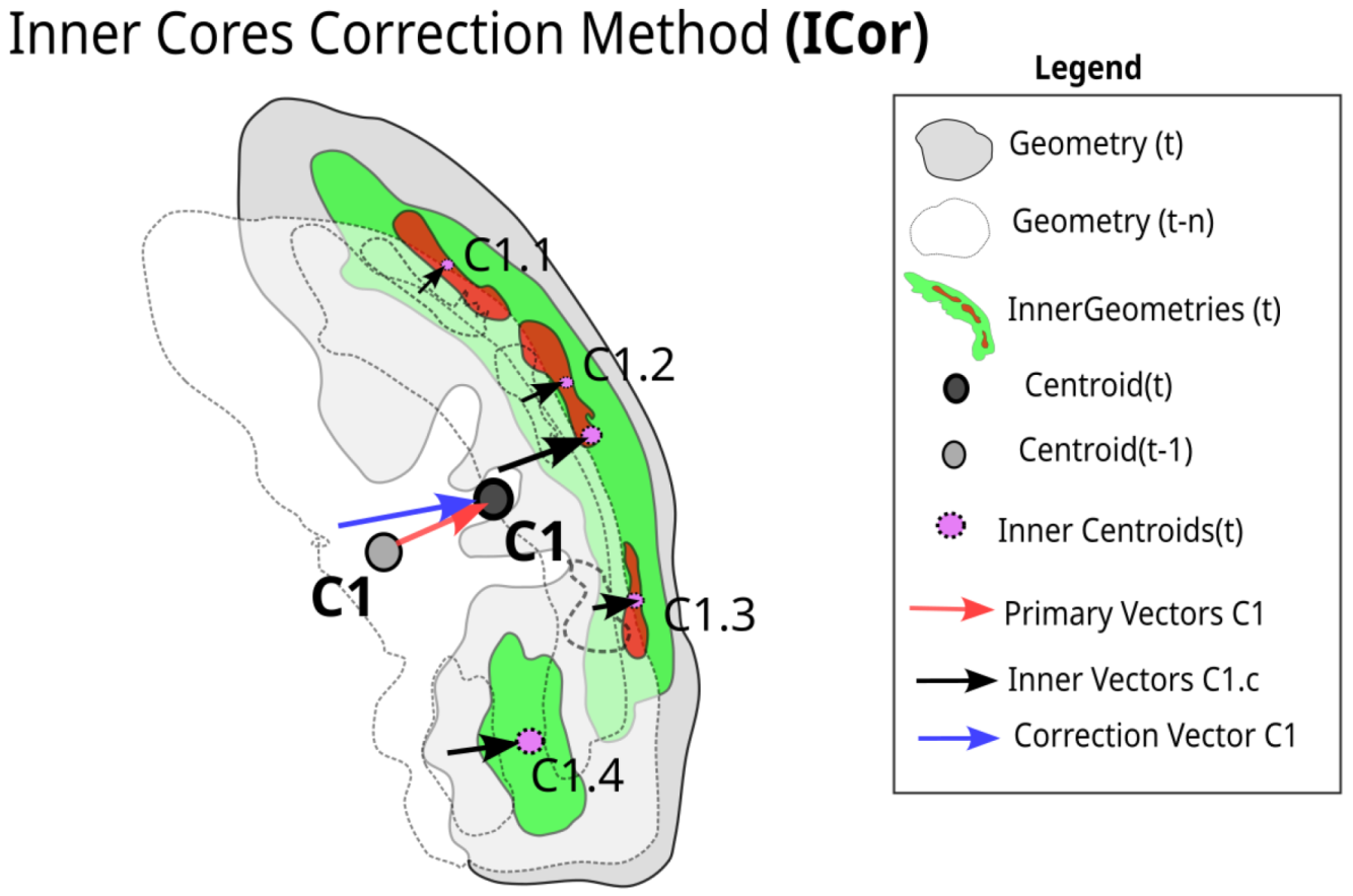
Correction by Rain Cell Inner Cores

As previously mentioned, a problem with changing the tracked system’s shape can appear in many different ways and abruptly. However, internal cores can represent a solution to this problem. Because they are smaller in area and displacement, the observed variations can better describe the system’s displacement at a given instant. In this case, a correction method using vectors associated with the Inner Cores (ICor) of the rain cells can be applied to correct the trajectory at the current time. This method outputs correction vectors associated with the displacement of the cell sorted by the first threshold at time t. Figure 7 illustrates how this method adjusts the displacement vector; the grey polygon represents the geometry of the primary threshold boundary, while smaller polygons (purple) represent geometries of internal thresholds (more intense reflectivity thresholds) and their respective displacement vectors. The adjusted vector (blue arrow) is the averaged vector (Equation (1)) related to the inner cores (black arrow). It replaces the primary vector related to the outer threshold (red arrow).

Combination

All the above methods act on a specific condition, sometimes trying to improve the split vector, sometimes the merges, among other things. However, in the same rain cell there are several conditions to applying different methods at the same time; in this case we also evaluate these groups (combinations), even counting how many times they occur (activation). In addition, there is still the fact that not all tracking problems were accounted for, not only for the lack of knowledge of all the questions that involve the tracking of rain cells, but for the fact that sometimes the vector to be corrected is in fact the most realistic one. So, all the above methods were combined with the uncorrected vector, here called “NONE”. Equation (1) was used to average the vectors for each combination shown in the following section.

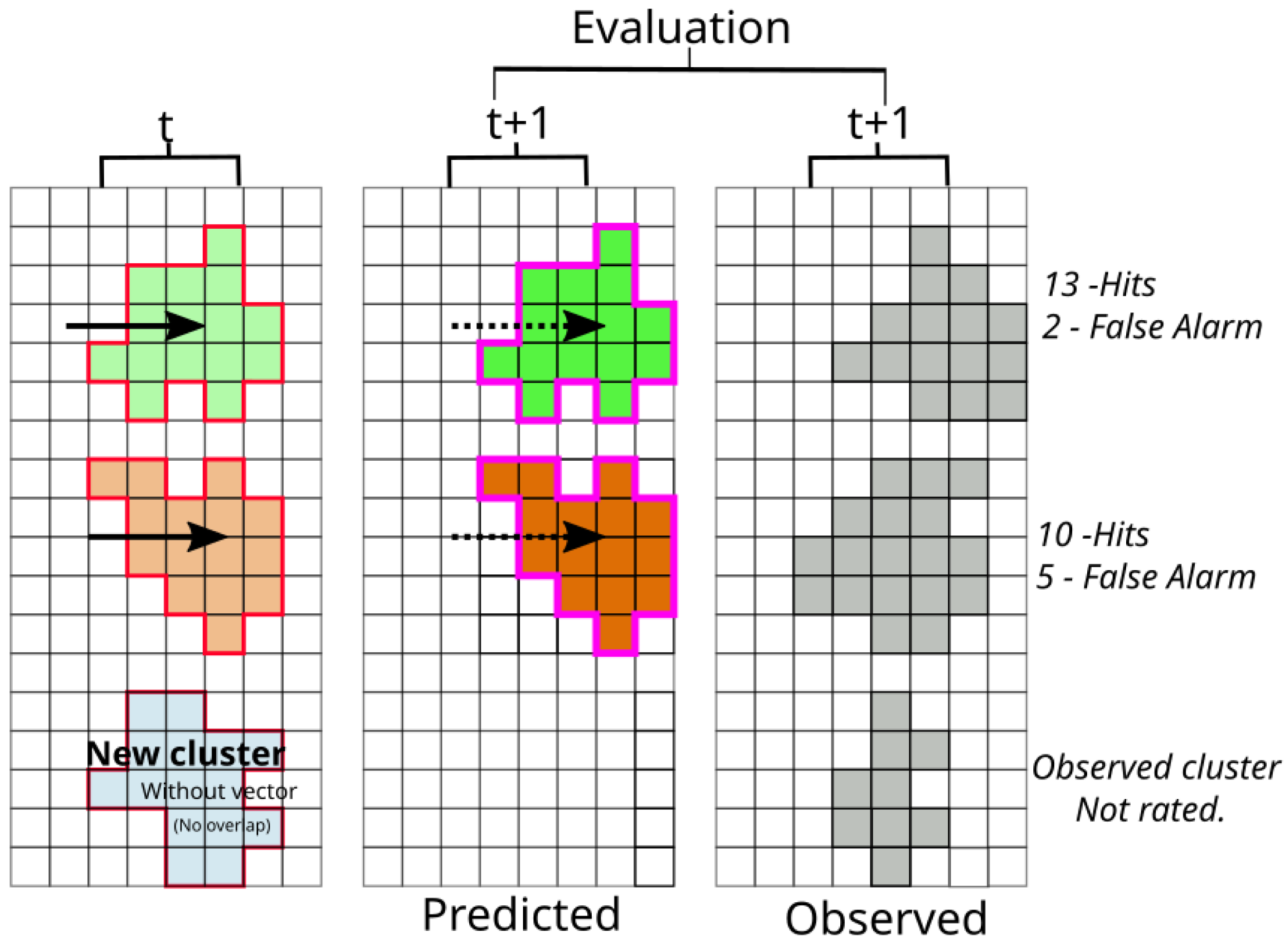
2.3. Validation by Persistence

As there is no reference of what would be the best method for tracking, the displacement correction methods have been evaluated by the persistence of the spatio-temporal extrapolation of the rain cell. That is, each method and combination will be evaluated to determine which performs best. During this process, the cluster at time t is extrapolated based on the velocity and direction values obtained by the method one time ahead and, if this same cluster is also observed at time $t+1$, the skill of the method for the current instant will be measured. All pixels of the cluster are shifted forward and thus form a persistent cell at $t+1$. This extrapolation of the cluster has its values evaluated dichotomously (true or false) with the observation one time ahead.

The extrapolation of the pixel values of each rain cell is displaced according to the direction and velocity values obtained by the methods. Figure 8 shows the validation of the extrapolation method. In order to determine the performance, the specific rain cell in a time step was isolated, that is, without the presence of the others in the entire radar image. Moreover, it is considered that the rain cell classified as new will not be used due to the lack of vector information for extrapolation. The results will show how the proposed corrections impact the forecasting results.

Finally, having established the extrapolation metrics, the evaluation performance for each correction method will be performed using the statistical prediction parameters [37], which are:

• Hit: When the rain pixel was predicted and observed.
• Miss: Rain pixel not predicted but observed.
• False Alarm: Predicted rain pixel that did not occur.
• Correct Negative: Rain pixels were not forecasted and also did not occur.

In addition to statistical prediction parameters, accuracy rates given by POD and FAR will also be considered to measure the prediction ability (Skill Score) between these rates for different corrections.

POD: This is a ratio between the number of correctly forecasted rain pixels and the number of observed ones. If all predictions are correct, the result of this operation is 1, and if all predictions are incorrect, the result is 0.

$$POD=\frac{Hit+Miss}{Miss}$$

(2)

FAR: The ratio of false alarms against the total number of expected rain pixels is used to calculate FAR. The perfect score for FAR is 0.

$$FAR=\frac{FalseAlarm}{Hit+FalseAlarm}$$

(3)

The values used in the Skill Score function are correlated with a reference value that will be the basis of comparison for the other vector correction and extrapolation methods. Therefore, the function to evaluate the skill of the methods is described as follows:

$$SkillScore=\frac{SkillScor{e}_{predicted}-SkillScor{e}_{reference}}{SkillScor{e}_{perfectscore}-SkillScor{e}_{reference}}\ast 100$$

(4)

3. Results

The results demonstrate aspects related to the tracking of precipitating systems during GoAmazon Intensive Operating Periods (IOP1 and IOP2). The analyses are designed to define the influence of thresholds on tracking and evaluate the application of these methods and their impact on correcting errors associated with rain cell geometry in the Amazon region.

3.1. The Minimum Size of Rain Cells

Before starting to proceed with the general evaluation of thresholds and correction methods, it is necessary to define the minimum cluster (rain cell) size parameter. Together with the external contour threshold parameter, the minimum size of rain cells can strongly affect the tracking and prediction. We initially selected reflectivity thresholds of 20, 30, and 35 dBZ based on previous studies [4,8,31,32,38] and evaluated the percentage of rain cells identified in the initial tracking period, i.e., the transition after the cluster identification and its time ahead ($t+1$). In order to identify the minimum cluster size which has a certain degree of continuity, only rain cells classified on the class transition from NEW to CON were analyzed. Figure 9 shows the percentage (%, line) of new rain cells with continuity and the respective number of cells tracked (bar chart) for each minimum size range (4 pixels; the last class groups all clusters larger than 100 pixels in size). It is clear in Figure 9 that for minimum sizes smaller than 15 pixels (60 km²) the number of rain cells increases considerably; however, the degree of continuity is small. Tracking of these precipitating systems is challenging because there is a small or no overlap between consecutive images, or because they have short lifetimes, or even because of false identification of rain cells.

It is notable that for intervals larger than 45 pixels (180 km²), the transition percentage of the rain cells does not have a pattern, which may be related to the low number of samples. For a threshold between 15 and 25 pixels, it is noted that there is a good degree of continuity (>40%) with a number of systems tracked that is sufficient for analyzing the effects of the proposed corrections. Because the InnerCores correction requires the existence of better developed internal structure, a minimum size of 25 pixels was chosen for the following analyses. However, in situations where this correction might not be needed, using 15 pixels would guarantee a larger number of tracked rainy systems.

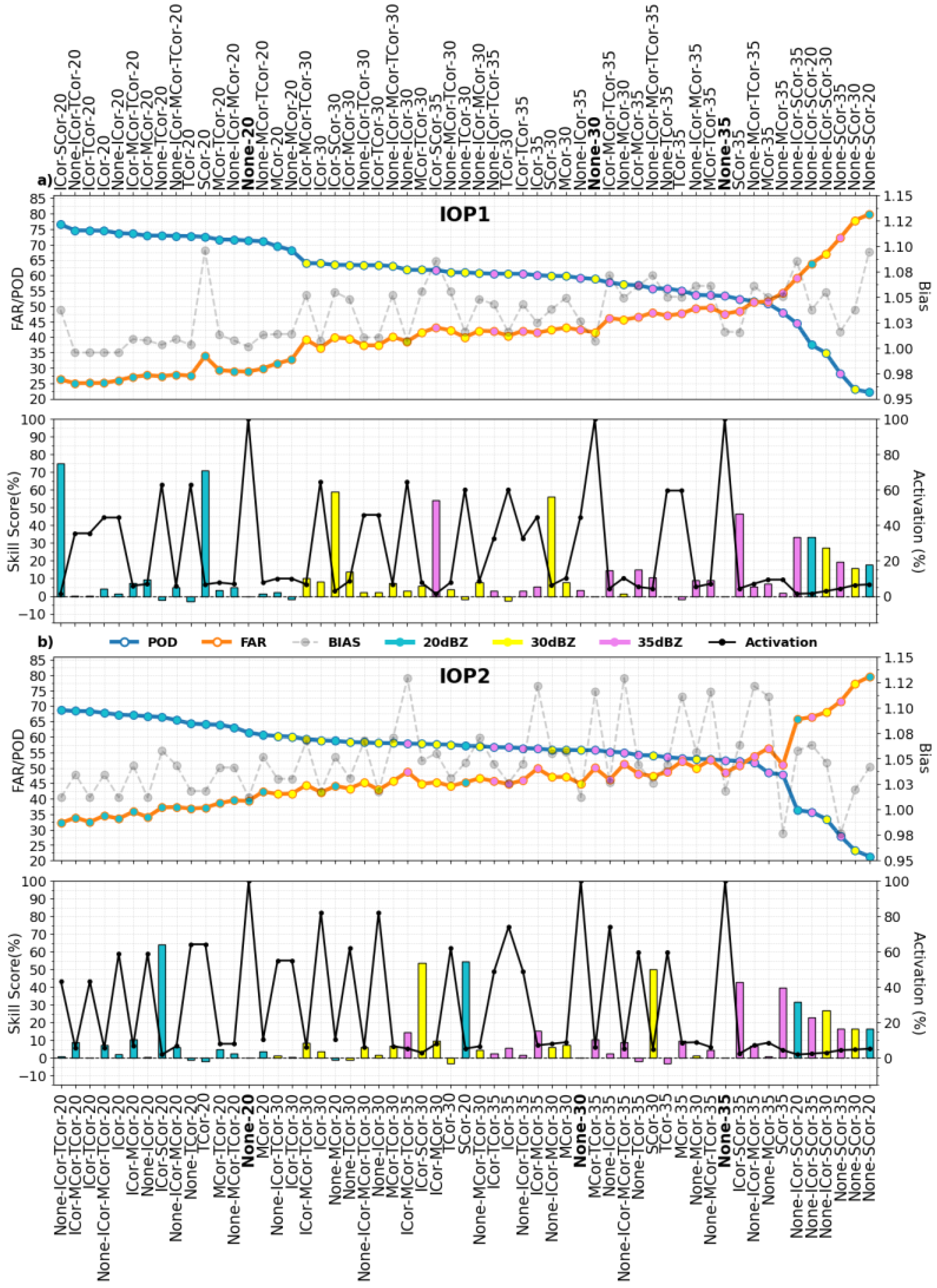
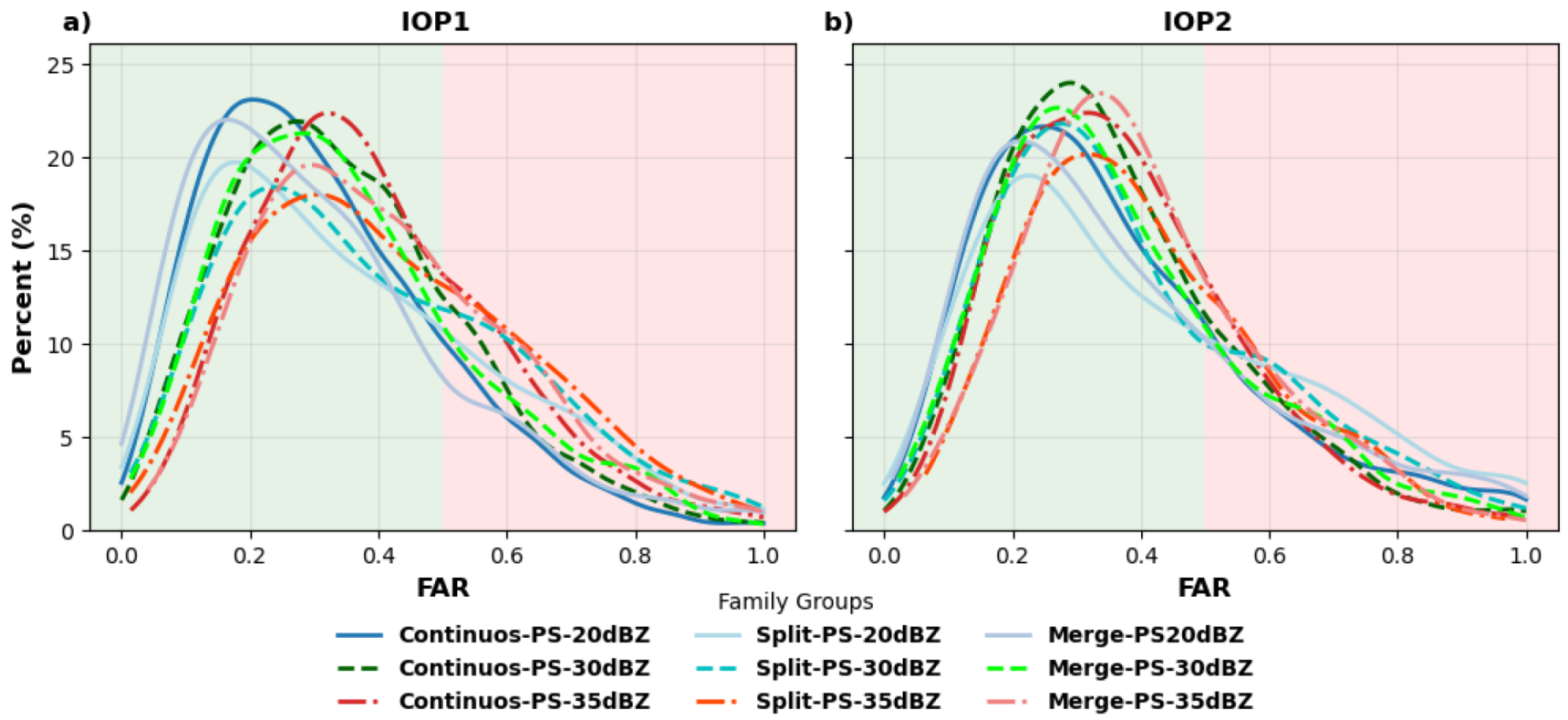
3.2. Evaluation of Vector Correction Methods

In order to evaluate all methods against reflectivity thresholds, the minimum size of rain cells was set to 25 pixels (thresholds of 20 dBZ), as described before, and the primary inner cores have at least 15 pixels (thresholds of 30 dBZ) and the secondary (thresholds of 35 dBZ) was 10 pixels. The choice of these values is associated with the observed rainfall characteristics [4,8,31,32,38]. The lower thresholds indicate lighter (20 dBZ) and moderate (30 dBZ) rainfall rates, while the latter (35 dBZ) refers to a condition associated with a probable convective initiation [39].

The evaluation of the methods is seen in Figure 10 which shows the values of averaged POD (%, blue line), FAR (%, orange line), and BIAS (gray line) based on the prediction of rain cell position at $t+1$. Results for each IOP are shown in separate panels, and the horizontal axis represents the combination of methods and their threshold (Method_Combination_Reflect). The skill score (%, colored bars) and activation frequency (Act.%, black lines) are shown on the adjacent panels, and indicate the improvements for the individual method (or combination) and how many times each one was used. Except for “NONE”, where the entire population of data was used (100%), the statistics shown only reflect the sample where each combination was applied. Moreover, the percentage of activation (number of rain cells divided by the total) where a certain combination occurred is shown in the bottom chart (Figure 10. Because of this, the percentage of activation (number of rain cells divided by the total) where a certain combination occurred is shown in the bottom chart. The activation frequency lines change as a function of the applied threshold. All tests without any corrections (called “NONE”) for each identification threshold (20, 30, and 35 dBZ) are represented on the x-axis in bold. As expected, some methods have been activated more than others. The reason for this is that different precipitating systems lead to the use of different correction methods for each time step during the life cycle. Moreover, this characteristic leads to a variety of POD, FAR, and BIAS, and should be considered when selecting the supposed best combination method. The order of the methods along the x-axis order was given only by the POD values of each method combination, where the best index (POD, FAR) is on the left of the graph and the worst on the right, for each IOP. To summarize these results,

Table 1. Number of associations of each method related to the best and worst combinations with respect to the algorithm without corrections in the displacement vector (None) for each threshold method.

			IOP1
	Better 20 dBZ	Worst 20 dBZ	Better 30 dBZ	Worst 30 dBZ	Better 35 dBZ	Worst 35 dBZ
ICor	9	1	9	1	9	1
TCor	7	1	8	0	7	1
MCor	5	3	7	1	5	3
None	5	4	6	3	5	4
SCor	2	2	2	2	1	3
Total Best Worst	13	5	15	3	12	6
			IOP2
	Better 20 dBZ	Worst 20 dBZ	Better 30 dBZ	Worst 30 dBZ	Better 35 dBZ	Worst 35 dBZ
ICor	9	1	9	1	7	3
TCor	8	0	8	0	8	0
MCor	6	2	7	1	6	2
None	6	3	6	3	5	4
SCor	1	3	1	3	0	4
Total Best Worst	13	5	14	4	12	6

shows the frequency of occurrence of a certain correction method in a combination that improves or worsens the POD/FAR with respect to the reference (“NONE”). It was divided by groups of the best (best at IOP1, best at IOP2), on the left of NONE in Figure 10, and worse (worse at IOP1, worse at IOP2), on the right of NONE in Figure 10, for each of the radar reflectivity thresholds.

Regarding the methods, as shown in both Figure 10 and Table 1, the ICor (i.e., inner thresholds) was the most activated one for all identification thresholds. As seen in Section 2.2.3, this method uses the internal clusters of the rain cell for vector correction. This was applied over 70% of the time depending on the threshold, followed closely by the TCor. On the other hand, MCor and SCor were used a few times, which shows that precipitation systems that occur only under these conditions are not frequent. However, the results indicate that, when observing systems with a more complex life cycle, where merges and splits occur and internal cores are observed, the applied corrections are effective, providing the best performance for IOP1 (POD = 76.51%, FAR = 26.22% and BIAS = 1.03) and IOP2 (POD = 68.65%, FAR = 32.15% and BIAS = 1.01) compared to NONE.

The differences between the methods for the same identification threshold are small, Figure 10. It can be observed in Table 1 that the lack of correction (NONE), even when it happens in a specific time step in combination with other corrections during the lifespan of the cell, still continues to cause more errors. The skill of each correction depends on the applied threshold, but they are generally beneficial to the tracking, particularly at higher thresholds. Moreover, there are slight differences in the activation of each correction between the two IOPs (Table 1); even if the precipitating systems have different physical characteristics throughout the life cycle in each period, their frequencies are proportional.

To evaluate the gains of each method individually, the skill score was computed comparing their results with the reference method (None) of its respective threshold. At the bottom, Figure 10a,b showed the gain and loss of each method (color bars). It is seen that in some methods there was a significant gain, with improvements of 75%, mostly for rain cells that used the split correction. This can be understood by the fact that many of the errors occur due to abrupt changes in velocity, and this correction tends to suppress large variations of the velocity. Moreover, it should be noted that while the skill gain of the method is high, its activation was relatively low, i.e., the method was used in few cases during the tracking but was highly effective.

The statistical indices of each method were directly affected by the identification threshold. Based on the POD/FAR values, it is possible to observe that the greater the radar reflectivity, the worse the performance of the model, especially during IOP2. This behavior may be associated with the physical characteristics of the systems tracked in each IOP, and with the fact that higher reflectivity thresholds correspond to smaller areas of the precipitating systems. During the wet season (IOP1), atmospheric systems in the Amazon region usually have lower precipitation rates [8] over larger areas, a characteristic of stratiform rain [7]. In contrast, a more significant number of severe storm cells is observed during IOP2, which is a dry season. Moreover, the performance of all correction methods is worse in IOP2. This result shows that the choice of tracking threshold should not be made arbitrarily, without understanding the characteristics of the precipitating systems in a given region. Even with most combinations bringing improvements, the tracking for more intense PSs (thresholds of 30 and 35 dBZ) is challenging.

As noted in the previous analysis, the combination depended on some physical aspects throughout the life cycles of the rain cells. It is likely that some characteristics associated with size and lifespan may be predominant factors in the use of certain correction methods. For instance the size can indicate a greater probability of mergers and splits, and the occurrence of more intense internal cores. In addition, with a longer lifetime, the probability of occurrence of merge and split increases as well, and also the use of corrections that take into account the temporal variation throughout the life cycle. Finally, it is expected that the tracked sizes decrease as the threshold increases, affecting the activation of a certain method. In order to investigate what these positive and negative impacts are during tracking for each interaction class, an analysis based on the average behavior of groups of tracked rainy systems was performed and is discussed in the next section.

3.3. Features That Most Impact Tracking Performance

In this section, the impact of corrections throughout the complete life cycle of the systems and depending on the different types of interactions (described in Section 2.3) is evaluated. The precipitating system refers to a set of rain cells (clusters) at different overlapping time steps that represent a single tracking. These precipitating systems were labeled according to the classes: Continuous-PS represented only by rain cells categorized as continuous (see Section 2.3); Merges-PS when only rain cells merging and continuities are observed; and Splits-PS when split and continuous rain cells are observed. In this study, only precipitating systems with at least three consecutive images (36 min) were analyzed.

The algorithm was applied with the same minimum size thresholds and all identification thresholds. However, it is important to make it clear that the 20 dBZ tracking is more suitable in the Amazon region for PSs in general. Furthermore, instead of choosing a specific combination of corrections, the algorithm applies the best-observed correction (the one with the smallest error) to each rain cell throughout its life cycle, called Adaptive. This choice was made in order to emphasize the impact of the physical characteristics of each precipitating system, reducing the effects of a specific correction.

Based on the correction (combinations) using the adaptive mode, Figure 11 shows the amount of rain cells corrected by their respective method for each threshold (bars: green for 20 dBZ, orange for 30 dBZ, and red for 35 dBZ) and both IOPs (IOP1, Figure 11a, IOP2, Figure 11b). As expected, the rain cell population without an effective correction method (NONE) is the majority (three times more than the second method). The remaining cells corrected by the adaptive mode are sorted in a descending manner, based on the IOP1 occurrence of the most used method/combination ordering (Figure 11). Although the number of rain cells at 20 dBZ of the TCor method is higher, the ICor method was more effective in the corrections for more intense thresholds, mainly for 35 dBZ. Some methods were not chosen in adaptive mode, as there was always a better one. This was the case for the “None-Icor-MCor-TCor” combination during IOP1 for 35 dBZ. Many of the methods smooth the displacement vector, such as TCor and SCor, and their results proved to be the best choice for several precipitating systems. In some cases, it may happen that the direction is correct, but the speed is not. Therefore, such methods prove to be effective as speed limiters, and when combined with NONE, they bring the best tracking option. The differences between the IOPs were small, which suggests that corrections can be applied similarly for both seasons. However, the skill is different, as will be shown in the next analysis.

As the adaptive mode was used, it is important to present its performance.

Table 2. Statistical indices by thresholds during the IOPs for the algorithm in adaptive mode.

		IOP1			IOP2
	20 dBZ	30 dBZ	35 dBZ	20 dBZ	30 dBZ	35 dBZ
POD	78.74%	67.96%	60.83%	68.60%	64.53%	61.11%
FAR	21.52%	32.53%	40.13%	32.30%	36.29%	39.98%
BIAS	1.0032	1.0073	1.0160	1.0132	1.0129	1.0182

presents the skills achieved using the algorithm in adaptive mode. We see that the lower intensity thresholds (20 dBZ) obtained the best POD, FAR, and BIAS indices. Moreover, during IOP1 the precipitating systems were better tracked than in IOP2, as observed before. This may be associated with difficulties in tracking more severe events. A slight improvement was observed overall for the adaptive method compared to choosing a specific combination, as can be seen in the values between Table 2 and Figure 10.

The rain cells were grouped into precipitating systems of a certain interaction class. It is important to show the number of occurrences of them.

Table 3. Occurrence of the precipitating system classes for each IOP and threshold.

		IOP1			IOP2
Precipitating System	20 dBZ	30 dBZ	35 dBZ	20 dBZ	30 dBZ	35 dBZ
Continuous	78.85%	81.07%	77.65%	75.60%	79.12%	78.28%
Merges	12.80%	10.51%	12.20%	13.64%	12.69%	12.97%
Splits	8.34%	8.41%	10.14%	10.76%	8.25%	8.74%

shows the percentages of the precipitating systems related to a certain class of interaction. Notably, PSs classified as continuous represent most of the cases. Merges (split) represent no more than 13.64% (10.76%) of the precipitating systems.

In order to analyze the positive and negative impacts of the best correction chosen throughout the life cycle of the cell, precipitating systems were also divided according to their general skills. That is, PSs that presented FAR values below (above) 0.5 (50%), regardless of the correction applied, showed better (worse) properties/conditions for tracking. Figure 12 shows the FAR relative frequency histogram of each PS tracked by their groups for the two IOPs and the threshold. It represents how the prediction of rain cells was distributed for each threshold and PS class during both IOPs. For this analysis, the false alarm rates of each PS class were pooled and a kernel density estimate (KDE) was applied based on the histogram of FARs. Note that the thresholds at 20 dBZ represented by the blue lines in Figure 12 indicate that the thresholds were closest to the best FAR (equal to 0). In contrast, the red lines, referring to the highest intensity threshold (35 dBZ), do not indicate a good performance, as already observed in a previous analysis. In general, the performance was better during IOP1 than for IOP2, with larger differences for 20 dBZ probably associated with a higher frequency of light rain cells during the wet season.

Two characteristics were analyzed in this study, which directly impact the tracking of non-rigid objects: the size and lifespan of each precipitating system. Figure 13 shows the boxplots related to the life cycle of groups with the best (≤0.5) and worst (>0.5) FAR indices. Regarding the lifespan, it is evident in the figure that Continuous-PSs are those with the shortest life cycle in general. Moreover, it is noted that the longer the system lifetime of the cell, the better the performance of the corrections. Comparing the two IOPs, the group with the best FAR indices has a longer lifetime in IOP2 than IOP1, in terms of the upper quartile, median, and average. In other words, systems during IOP2 need to have a slightly longer lifetime than those of IOP1 to have the same tracking performance, except for the Merge-PS-20 dBZ during IOP1, where the larger PSs proved to be more difficult to correct. A reason for this later result would be that merging of rain cells in IOP1 (larger clusters than IOP2) can suffer drastic changes.

When evaluating the average size of the rain cells for each precipitating system, it can be observed in the boxplots of Figure 14 (the same as in Figure 13, except for size) that the difference between the best-corrected individual groups (Figure 14a) leans towards presenting slightly larger rain cells, especially during IOP1. Moreover, it is possible to establish that the precipitating system classes with greater rain cell interaction (Split and Merge) obtained better results, especially during IOP1. The boxplots related to this season show that the mean, median, and upper quartiles present PSs with larger sizes in comparison to IOP2. This behavior becomes more evident for rain cells with lower thresholds where according to [8] less intense reflectivities are associated with larger stratified areas over the region. Such results demonstrate that the corrections are intrinsically dependent on the interactions between rain cells that occur throughout the life cycle of the PSs and that the thresholds directly impact this behavior. However, for systems with longer lifetime and size, the corrections applied proved to be effective.

4. Conclusions

Tracking algorithms are very important tools in monitoring meteorological events, and are especially useful for following precipitating cells. They can be used to help understand the evolution of rainy systems, and hence advance our knowledge about this key aspect of the climate system. In this sense, this study evaluated how to best correct the displacement of precipitating cells and how their intensity and size can impact our ability to track these systems in a specific region. Such a tool can be used to assess the development of weather systems, study their characteristics over the years, and even perform nowcasting of different weather systems with multiple data sources.

Here we reported on the use of the physical and dynamic characteristics of the precipitating systems to develop a new algorithm, which allowed the evaluation of several factors related to the precipitating systems that occurred in the two contrasting seasons. We proposed four different methods and their combination for correcting the displacement vector calculated between consecutive images that accounts for splits, merges, and other typical problems in tracking algorithms. When applying these correction methods and investigating the impact generated on the tracking of precipitating systems, it was found that there were improvements compared to the algorithm settings without any correction of the displacement vectors. In general, the POD indices for less intense (20 dBZ) thresholds were greater than 78.74% during IOP1 and 68.6% for IOP2, as shown in Table 2. These indices show that there was a good correction of the rain cells during the two seasons. However, the skill decreases towards higher reflectivity thresholds. The results obtained show that less intense thresholds better represent the propagation characteristics of the precipitating systems over the Amazon region.

Among all the methods that had the best performances, those combinations that used correction associated with interactions between cells (i.e., split, merge, and inner cores) were more prominent. The combinations with the corrections by internal cores were efficient for both IOPs, the corrections by zplit were more useful on IOP1, while for IOP2 the merge brought more improvements to the tracking. However, the number of activations of these methods (applied to merge and splits) is small, as these systems represent less than 20% of tracked systems. For the most activated methods, the correction by internal cores proved to be very efficient. This indicates that the most intense cores within the cloud dictate the displacement of the rain cell in general.

In general, most combinations brought improvements to tracking. However, some physical aspects can directly impact the choice of method and its skill. In this sense, we analyzed how the size of the systems and their life cycle impact the correction. Therefore, the algorithm was adjusted to choose the best prediction among all available method combinations in order to analyze only the physical aspects. The so-called adaptive mode showed slightly better results than using just a specific combination. The most used combinations were associated with corrections that limited the speed of the system, thus correcting the main problems of using the centroid. The uncorrected vector was often combined with corrective methods, which may be associated with the fact that it is not always completely wrong. The analyses accounted for all tracked rain cells. Moreover, the lack of knowledge about all possible correction hypotheses can be overcome using the combination with the uncorrected vector. It was possible to define that the corrections had better results when rain cells were larger and had a longer life cycle. During the dry season (IOP2), where rainy cells tend to be more intense, it is necessary that the lifetime is even longer to reach FAR value found during IOP1. Short-lived continuous precipitating systems are the majority of those tracked. Therefore, it is necessary to give greater priority in future work to such systems in order to improve monitoring in general, especially in the initiation and shallow convection.

Based on these results, it is possible to say that the corrections analyzed improved the tracking of precipitating systems over the Amazon region. Furthermore, the combination of these different methods is the best approach for monitoring precipitating systems in the Amazon region, especially if there are two or more seasons with different characteristics. In addition, the definition of the threshold and minimum size of the tracked systems are factors that directly impact the skill of the algorithms and must be determined from the common physical characteristics of all rain events in a region, a well-known aspect in nowcasting strategies [9]. Therefore, it is suggested that for the monitoring of meteorological events, the algorithm should be adaptive to the observed features of each rain cell throughout their lifespan and frequency. Furthermore, it is important for decision-makers to know that depending on these characteristics, certain precipitating systems are better monitored than others.

In future work, data from different sources will be used to improve the tracking of the precipitating systems and increase the study coverage area (radar data is limited to 480 × 480 km). Such research will focus on the fact that no analysis in this study was done considering that some precipitating systems may be larger than the radar coverage area, which can bring uncertainty to the applied corrections. Moreover, it is worth mentioning that this study uses persistence as a basis to validate its correction methods. Therefore, there are uncertainties associated with the forecast in all verification analyses that were not taken into account. However, the results are believed to be robust enough due to the short time difference between consecutive images (12 min). In future works, research will be addressed to study the sensitivity of persistence in the intercomparison between similar tracking algorithms. In addition, studies for other regions of the globe will be carried out to validate the aspects that most impact nowcasting for different storms depending on the environment that surrounds them.

References

- Marengo, J.A.; Nobre, C.A. General characteristics and variability of climate. In The Amazon Basin and Its Links to the Global Climate System the Biogeochemistry of the Amazon Basin; Oxford University Press: New York, NY, USA, 2001; ISBN 978-01-9511-431-7. [Google Scholar]
- Fisch, G.; Marengo, J.A.; Nobre, C.A. On the hydrological cycle of the Amazon Basin: A historical review and current state-of-the-art. SciELO Bras. Acta Amaz. 1998, 28, 101. [Google Scholar] [CrossRef]
- Garstang, M.; Ulanski, S.; Greco, S.; Scala, J.; Swap, R.; Fitzjarrald, D.; Martin, D.; Browell, E.; Shipman, M.; Connors, V.; et al. The Amazon boundary-layer experiment (ABLE 2B): A meteorological perspective. Bull. Am. Meteorol. Soc. 1990, 71, 19–32. [Google Scholar] [CrossRef]
- Laurent, H.; Machado, L.A.; Morales, C.A.; Durieux, L. Characteristics of the Amazonian mesoscale convective systems observed from satellite and radar during the WETAMC/LBA experiment. J. Geophys. Res. Atmos. 2002, 107, LBA-21. [Google Scholar] [CrossRef]
- Cohen, J.C.P.; Silva, D.M.A.F.; Nobre, C.A. Aspectos climatológicos das linhas de instabilidade na Amazônia. Climanálise 1989, 4, 34–40. [Google Scholar]
- Chalon, J.P.; Jaubert, G.; Lafore, J.P.; Roux, F. The West African squall line observed on 23 June 1981 during COPT 81: Mesoscale structure and transports. Am. Meteorol. Soc. J. Atmos. Sci. 1988, 45, 2744–2763. [Google Scholar] [CrossRef]
- Houze, R.A. Structure and dynamics of a tropical squall–line system. Am. Meteorol. Soc. Mon. Weather Rev. 1977, 105, 1540–1567. [Google Scholar] [CrossRef]
- Machado, L.A.; Calheiros, A.J.; Biscaro, T.; Giangrande, S.; Silva Dias, M.A.; Cecchini, M.A.; Albrecht, R.; Andreae, M.O.; Araujo, W.F.; Artaxo, P.; et al. Overview: Precipitation characteristics and sensitivities to environmental conditions during GoAmazon2014/5 and ACRIDICON-CHUVA. Copernic. GmbH Atmos. Chem. Phys. 2018, 18, 6461–6482. [Google Scholar] [CrossRef] [Green Version]
- WMO (World Meteorological Organization). Guidelines for Nowcasting Techniques. Available online: https://library.wmo.int/doc_num.php?explnum_id=3795 (accessed on 12 September 2022).
- Crane, R.K. Automatic cell detection and tracking. IEEE Trans. Geosci. Electron. 1979, 17, 250–262. [Google Scholar] [CrossRef]
- Vila, D.A.; Machado, L.A.; Laurent, H.; Velasco, I. Forecast and Tracking the Evolution of Cloud Clusters (ForTraCC) using satellite infrared imagery: Methodology and validation. Weather Forecast. 2008, 23, 233–245. [Google Scholar] [CrossRef]
- Dixon, M.; Wiener, G. TITAN: Thunderstorm identification, tracking, analysis, and nowcasting—A radar-based methodology. Weather Forecast. 1993, 10, 785–797. [Google Scholar] [CrossRef]
- Sawant, M.; Shende, M.K.; Feijóo-Lorenzo, A.E.; Bokde, N.D. The State-of-the-Art Progress in Cloud Detection, Identification, and Tracking Approaches: A Systematic Review. Energies 2021, 14, 8119. [Google Scholar] [CrossRef]
- Aggarwal, J.K.; Cai, Q.; Liao, W.; Sabata, B. Articulated and elastic non-rigid motion: A review. In Proceedings of the 1994 IEEE Workshop on Motion of Non-rigid and Articulated Objects, Austin, TX, USA, 11–12 November 1994; pp. 2–14. [Google Scholar]
- Storlie, C.B.; Lee, T.C.M.; Hannig, J.; Nychka, D. Tracking of multiple merging and splitting targets: A statistical perspective. Stat. Sin. 2009, 19, 1–31. [Google Scholar]
- Zan, B.; Yu, Y.; Li, J.; Zhao, G.; Zhang, T.; Ge, J. Solving the storm split-merge problem—A combined storm identification, tracking algorithm. Atmos. Res. 2019, 218, 335–346. [Google Scholar] [CrossRef]
- Muñoz, C.; Wang, L.; Willems, P. Enhanced object-based tracking algorithm for convective rain storms and cells. Atmos. Res. 2021, 201, 144–158. [Google Scholar] [CrossRef]
- Lakshmanan, V.; Smith, T. An objective method of evaluating and devising storm-tracking algorithms. Am. Meteorol. Soc. Weather Forecast. 2010, 25, 701–709. [Google Scholar] [CrossRef]
- Han, L.; Fu, S.; Zhao, L.; Zheng, Y.; Wang, H.; Lin, Y. 3D convective storm identification, tracking, and forecasting—An enhanced TITAN algorithm. J. Atmos. Ocean. Technol. 2009, 26, 719–732. [Google Scholar] [CrossRef]
- Sieglaff, J.; Hartung, D.; Feltz, W.; Cronce, L.; Lakshmanan, V. A satellite-based convective cloud object tracking and multipurpose data fusion tool with application to developing convection. Am. Meteorol. Soc. J. Atmos. Ocean. Technol. 2013, 30, 510–525. [Google Scholar] [CrossRef]
- Leal Neto, H.B.; Almeida, A.P.; Calheiros, A.J.P. As dificuldades no rastreio de tempestades com uso de refletividade radar a partir de técnicas de geoprocessamento: Um estudo de caso sobre a região Amazônica. In Proceedings of the XXI GeoInfo, Sao Jose dos Campos, Brazil, 30 November–3 December 2020; pp. 240–245. [Google Scholar]
- Anselmo, E.M.; Machado, L.A.T.; Schumacher, C.; Kiladis, G.N. Amazonian mesoscale convective systems: Life cycle and propagation characteristics. Int. J. Climatol. 2021, 41, 3968–3981. [Google Scholar] [CrossRef]
- Machado, L.A.T.; Rossow, W.B.; Guedes, R.L.; Walker, A.W. Life cycle variations of mesoscale convective systems over the Americas. Mon. Weather Rev. 1998, 126, 1630–1654. [Google Scholar] [CrossRef]
- Schumacher, C.; Funk, A. GoAmazon2014/5 Rain Rates from the SIPAM Manaus S-band Radar. 2018. Available online: https://www.osti.gov/dataexplorer/biblio/dataset/1459578 (accessed on 14 July 2022).
- Martin, S.; Artaxo, P.; Machado, L.; Manzi, A.O.; Souza, R.A.F.; Schumacher, C.; Wang, J.; Biscaro, T.; Brito, J.; Calheiros, A.; et al. The Green Ocean Amazon Experiment (GoAmazon2014/5) Observes Pollution Affecting Gases, Aerosols, Clouds, and Rainfall over the Rain Forest. Bull. Amer. Meteor. Soc. 2017, 98, 981–997. Available online: http://journals.ametsoc.org/doi/abs/10.1175/BAMS-D-15-00221.1 (accessed on 25 October 2022). [CrossRef] [Green Version]
- Rinehart, R.E.; Garvey, E.T. Three-dimensional storm motion detection by conventional weather radar. Nature 1978, 273, 287–289. [Google Scholar] [CrossRef]
- Fiolleau, T.; Roca, R. An algorithm for the detection and tracking of tropical mesoscale convective systems using infrared images from geostationary satellite. IEEE Trans. Geosci. Remote Sens. 2013, 51, 4302–4315. [Google Scholar] [CrossRef]
- Shehu, B.; Haberlandt, U. Improving radar-based rainfall nowcasting by a nearest-neighbour approach–Part 1: Storm characteristics. Copernic. GmbH Hydrol. Earth Syst. Sci. 2022, 26, 1631–1658. [Google Scholar] [CrossRef]
- Foresti, L.; Sideris, I.V.; Nerini, D.; Beusch, L.; Germann, U. Using a 10-year radar archive for nowcasting precipitation growth and decay: A probabilistic machine learning approach. AMS Weather Forecast. 2019, 34, 1547–1569. [Google Scholar] [CrossRef]
- Doyle, W. Operations useful for similarity-invariant pattern recognition. J. ACM (JACM) 1962, 9, 259–267. [Google Scholar] [CrossRef]
- Nunes, A.M.P.; Silva Dias, M.A.F.; Anselmo, E.M.; Morales, C.A. Severe convection features in the Amazon Basin: A TRMM-based 15-year evaluation. Front. Earth Sci. 2016, 4, 37. [Google Scholar] [CrossRef] [Green Version]
- Eichholz, C.W. Kinematic and Dynamic Analysis of Rain and Cloud Cells Propagation. Ph.D. Thesis, Instituto Nacional de Pesquisas Espaciais, Sao Jose dos Campos, Brazil, May 2017. Available online: http://urlib.net/rep/8JMKD3MGP3W34P/3NQ5D2P (accessed on 10 August 2022).
- Ester, M.; Kriegel, H.; Sander, J.; Xu, X. A Density-Based Algorithm for Discovering Clusters in Large Spatial Databases with Noise. In Proceedings of the Second International Conference on Knowledge Discovery and Data Mining, Portland, OR, USA, 2–4 August 1996; pp. 226–231. [Google Scholar]
- Matthews, J.; Trostel, J. An Improved Storm Cell Identification and Tracking (SCIT) Algorithm based on DBSCAN Clustering and JPDA Tracking Methods. American Meteorological Society. 2010. Available online: https://ams.confex.com/ams/pdfpapers/164442.pdf (accessed on 10 August 2022).
- Garstang, M.; Massie, H.L.; Halverson, J.; Greco, S.; Scala, J. Amazon coastal squall lines. Part I: Structure and kinematics. Mon. Weather Rev. 1994, 122, 608–622. [Google Scholar] [CrossRef]
- Cotton, W.R.; Anthes, R.A. Storm and Cloud Dynamics; Academic Press: Cambridge, MA, USA, 1992. [Google Scholar]
- Wilks, D.S. Forecast Skill. In Statistical Methods in the Atmospheric Sciences; Academic Press: Cambridge, MA, USA, 2011; Volume 100, pp. 259–269. [Google Scholar]
- Machado, L.A.T.; Laurent, H. The convective system area expansion over Amazonia and its relationships with convective system life duration and high-level wind divergence. Mon. Weather. Rev. 2004, 132, 714–725. [Google Scholar] [CrossRef]
- Austin, P.M. Relation between measured radar reflectivity and surface rainfall. Am. Meteorol. Soc. Mon. Weather. Rev. 1987, 115, 1053–1070. [Google Scholar] [CrossRef]