Abstract
The occurrence of forest fires has increased significantly in recent years across the planet. Events of this nature have resulted in the leveraging of new automated methodologies to identify and map burned areas. In this paper, we introduce a unified data-driven framework capable of mapping areas damaged by fire by integrating time series of remotely sensed multispectral images, statistical modeling, and unsupervised classification. We collect and analyze multiple remote-sensing images acquired by the Landsat-8, Sentinel-2, and Terra satellites between August–October 2020, validating our proposal with three case studies in Brazil and Bolivia whose affected regions have suffered from recurrent forest fires. Besides providing less noisy mappings, our methodology outperforms other evaluated methods in terms of average scores of 90%, 0.71, and 0.65 for overall accuracy, F1-score, and kappa coefficient, respectively. The proposed method provides spatial-adherence mappings of the burned areas whose segments match the estimates reported by the MODIS Burn Area product.
1. Introduction
Climate change is one of the most significant environmental challenges facing humanity. Occasionally, these changes in climate increase the probability of extreme events that alter rainfall and drought patterns [1,2] in several regions of the planet, besides triggering the process of natural disasters arising mainly from floods, landslides, droughts, and forest fires [3].
Extreme droughts are among the worst climatic disasters since they produce large economic and social losses [4,5]. Moreover, these phenomena also cause forest fires [6], an environmental issue that has been observed over the years, leading to severe ecological damages [7]. Frequent fires are hazardous because they affect forest regeneration, making fire a disruptive agent of this environment’s dynamics [8]. Consequently, fire mapping and its monitoring are essential to detect, mitigate, and even prevent harmful impacts [9,10].
Aiming at addressing this issue, one can apply remote sensing (RS) technologies, which gather a comprehensive collection of multitemporal data and effective imaging products. In fact, new RS-driven computational apparatuses have been proposed in the last years, enabling the extraction of high-quality data over vast monitored regions with high temporal frequency and reasonable operational costs [11]. Moreover, the development of new and more accurate data-driven tools for tracking, monitoring, and predicting fire events is leveraged in both the amount and quality of RS data, as continuously provided by a variety of sensors [12,13].
Considering the particular application of fire detection using RS data, several techniques have been created to obtain data from the Earth’s surface while mapping burned areas [14,15]. According to Birch et al. [16], the use of time series of images obtained by remote sensing is essential for studies about monitoring, management, and recovery of burned areas. In more computational terms, spectral indices as well as supervised machine-learning methods can be properly combined to produce representative detection maps for the fire. For instance, Gibson et al. [17] proposed a methodology that unified spectral indices taken from Sentinel-2, and used the random forest algorithm to map the burning severity in fire-affected areas. Similarly, Mohajane et al. [18] employed a historic forest fire inventory, composed of both local and environmental variables, to formulate distinct frequency-ratio machine learning-based methods for generating maps of fire risk areas. The creation of fire susceptibility maps was also the goal of Tien Bui et al. [19], whose authors introduced a kernel logistic regression model by taking in situ data. An extensive study by Collins et al. [20] discussed the training data requirements for adequately modeling the random forest method applied to distinguish burned areas. Likewise, Pacheco et al. [21] compared the K-nearest neighbor and random forest methods concerning the resulting burning maps using as input data images recorded by the sensor Operational Land Imager (OLI), Multispectral Instrument (MSI), and Moderate-Resolution Imaging Spectroradiometer (MODIS) on-board the satellites Landsat-8, Sentinel-2, and Terra/Aqua, respectively.
Concerning proposals that have applied spectral indices for fire mapping, recently Lasaponara et al. [10] proposed a self-organizing map-driven approach that relies on popular spectral indices, which include Normalized Difference Vegetation Index (NDVI), Normalized Burn Ratio (NBR), and Burned Area Index for Sentinel (BAIS), to enhance and identify burned areas. Mallinis et al. [22] analyzed the correlation between field survey measures and spectral indices computed from images acquired by the MSI and OLI sensors. By taking the difference Normalized Burn Ratio (NBR) [23] and its relative NBR (RNBR) [24] for fire mapping applications, Cai and Wang [25] performed a statistical analysis to demonstrate that the NBR index is more accurate and reliable than the RNBR for burn severity classification. Gholinejad and Khesali [26] employed the NDVI and Normalized Difference Water Index (NDWI) to first identify regions subjected to burning events and then run a change-point procedure based on NBR values to find a convenient threshold to distinguish burned areas. Mapping burned areas has not only been restricted to orbital sensors. For instance, McKenna et al. [27] adopted images recorded by unmanned aerial vehicle and the band indices excess green index, excess green index ratio, and modified excess green index to train a decision model for identifying distinct burn severity classes.
Fire detection has also been performed from the deep-learning perspective. More recently, Hu et al. [28] took deep-learning strategies for the identification of regions impacted by fire by handling uni-temporal OLI and MSI images. By employing a deep learning-based formulation, Ba et al. [29] took an empirical spectral index based-rule to automatically select samples and model a back-propagation neural network to distinguish burned areas from native vegetation on MODIS images. Similarly, Ban et al. [30] took neural networks as a primary tool to perform the mapping of wildfires. In a simple but efficient way, Matricardi et al. [31] proposed the use of probabilistic models to estimate canopy cover and fire potential in forest areas.
Despite the development of new data-driven algorithms for the detection and quantification of wildfires, the literature still lacks methods designed to classify wildfires automatically while ensuring high accuracy in the punctual mapping [30]. Indeed, for most supervised learning methods, obtaining a representative set of ground-truth data samples or a sizable number of annotated images for training are difficult tasks to accomplish in practice [32,33,34]. Another critical issue frequently found in most fire detection algorithms is that they are prone to failure when coping concurrently with temporal data, lighting conditions, and spectral bands’ complexity [35], a condition also present and addressed in other related remote sensing applications [36]. Finally, as highlighted by Khosravi et al. [37] and Barmpoutis et al. [32], there is no definitive data-driven approach that is optimal for hazard mappings, as the dependence on the study area and the availability of data can make most fire detection methods inoperative for hazard assessment.
Aiming at addressing most of the issues raised above, this paper introduces a novel data-driven multitemporal methodology for mapping burned areas by combining remote-sensing data and probabilistic models, identifying and classifying targets according to their changes measured in terms of the NBR index. These changes are turned into a mapping of burned areas by a fully unsupervised approach that applies logistic regression and spatial smoothing with Markov random fields modeling.
In summary, the introduced method comprises:
- A fully unsupervised methodology that unifies spectral indices, logistic regression, and Markov fandom fields into a spatial–temporal representation of burned areas;
- The proposed approach is capable of dealing with data acquired by sensors with distinct spatial radiometric resolutions;
- The proposed methodology retains some desirable features such as classification accuracy for images composed of different spatial resolutions, capability to handle severe imaging conditions such as cloud/shadow occurrences, and stability w.r.t. the systematic fire mapping task.
- Our computational approach is modular and, thus, flexible enough to be integrated with other learning models.
In our assessments, three case studies were carried out in regions located in Brazil and Bolivia using OLI, MSI, and MODIS images. Our choices were motivated by the fact that these study regions have suffered frequent fire events in recent years.
This article is organized as follows. Section 2 provides a brief review of fundamental concepts and techniques required for the proposed method, which is formalized in Section 3. Section 4 presents the application of the proposed method to map burned areas in three distinct areas using different sensors. Finally, Section 5 concludes this article.
2. Background
2.1. Definitions and Notation
Let be an image defined on the support acquired at an instant t, be the set of possible values at each position, and the observation at position of . In the remote-sensing context, the components of are the values measured by the sensor, or derived features, over a specific Earth surface position.
2.2. Spectral Indexes for Burnt Area Detection
Spectral indices allow the extraction and analysis of remotely sensed data. In the face of a feature of interest, a spectral index can assist in its identification. This approach is also essential due to the impossibility of modifying orbiting imaging sensors and the difficulty of obtaining field data with the same spatial and temporal resolution [38]. Generally speaking, spectral indices are derived from algebraic operations on the attributes of that characterize the behavior of at every pixel of .
Among dozens of spectral indices in the literature [39], typical examples are the NDVI [40], the NDWI [41], and the Soil Adjusted Vegetation Index (SAVI) [42].
Usually, such indices combine the information from visible (VIS), near-infrared (NIR), and shortwave-infrared (SWIR) spectral bands, being sensitive to variations in color, composition, soil moisture, and vegetation chlorophyll. The NBR [23] is a convenient index to identify burned areas.
Consider an image with and as components of the attribute vector , which represents the target behavior at position with respect to the NIR and SWIR wavelengths; the image of NBR values is defined as:
Spectral indices may be used at a single time t or as a time series. In the latter case, the use of differences between instants may help with identifying and mapping specific events. When the interest is mapping burned areas through remote-sensing images, the approaches found in the literature use only post-fire images or combine pre- and post-fire data [43]. In particular, Key and Benson [23] propose the “Delta-NBR” feature (), aimed at measuring the severity of fire events on the vegetation. Such methodology comprises a characterization of fire severity through the following difference:
where and are the NBR index computed at two distinct instants, before and after the fire event. Burning signs are usually characterized by values above . Table 1 displays a fire severity categorization proposed by Key and Benson [23].

Table 1.
Burning severity categorization.
Although the offers good perspectives regarding the fire severity effects on the landscapes, it is important to highlight that atmospheric interference, or even variations in the limits of NIR and SWIR spectral bands, may require adjustments in the burn severity categories (Table 1). Another limitation stems from the intrinsic features of each ecosystem, which may impose significant mismatches between the severity classes and those intervals [44].
We avoid the aforementioned limitations by building a binary map that incorporates both radiometric-derived and contextual information. The former enters through a logistic regression (Section 2.3); the latter uses the Iterated Conditional Modes (ICM) algorithm (Section 2.4).
2.3. Logistic Model
Logistic regression has been widely used to estimate the probability of membership in “element-classes” in cases of binary association [45]. It acts as a class indicator provided a set of observations , where .
This regression belongs to the class of generalized linear models [46], in which the response follows a Bernoulli law with probability of success
where is the parameter vector with one dimension more than the input vector and is a column of ones. The behavior of due to its sigmoid structure has an image defined in the range .
Beyond regression purposes, the model may also be applied for binary classification tasks. Equation (4) represents the classification result resulting from applying f on each position of :
where the values 0 and 1 are class indicators.
The parameter that characterizes f can be estimated by minimizing the following objective function [47]:
Although the derivative of (5) with respect to does not have an explicit form, its convexity grants that optimization algorithms such as the descending gradient converge to a global minimum [48].
2.4. Iterated Conditional Modes
The ICM algorithm is a classification technique that incorporates both the site evidence and the local information [49]. It is based on modeling the former with a suitable marginal distribution and the latter with a Markov random field for the underlying (unobserved) classes. It consists of solving the following maximization problem [50]:
where denotes , weights the influence of neighboring pixels (the context), is a clique (a clique of an undirected graph is a set of vertices such for all , there is an edge between i and j) that contains i, W is the set of cliques, is the coordinate set of neighboring pixels of , and
is the Kronecker delta function. Equation (6) is solved iteratively until a convergence criterion is met. The parameter is estimated, at each iteration, by maximum pseudolikelihood using the previous classification as input; see details in Frery et al. [50]. In the limit , the solution of (6) is the maximum likelihood classification map, while when , the observations are discarded in favor of the most frequent class in the neighborhood.
3. Method Proposal
3.1. Conceptual Formalization
Figure 1 depicts a high-level overview of the proposed method for burned area detection.
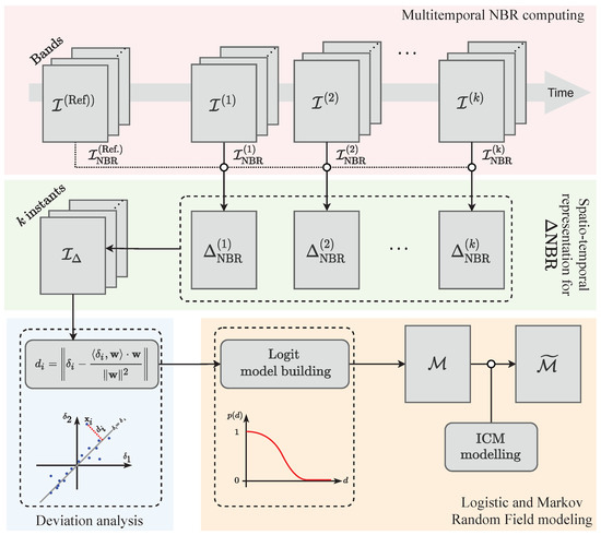
Figure 1.
Proposed method workflow.
3.1.1. Multitemporal NBR Computing
The red block outlines how the NBR is computed. Initially, assume there is a reference image expressing the usual behavior of targets regarding a spatial domain . Furthermore, let , for , be a multitemporal image series also regarding . Given , denote , for as an attribute vector with measures registered at n spectral wavelengths. Using the appropriate components of , it is possible to compute the NBR index at each position of and then determine .
3.1.2. Spatio-Temporal Representation for
The comprises a derived spectral index obtained by the difference of NBR at “pre” and “post” instants, in order to distinguish burn-affected or recovered burnt vegetation from other targets. In this sense, fixing as a “pre-fire event” image, we define for . We denote . Following the temporal order , the computed are combined to determine . In this representation, for a given , we have . These operations are represented in the “Spatio-temporal representation for ” block (Figure 1, green box).
3.1.3. Deviation Analysis
It is worth observing that is a spatio-temporal representation for the values. Locations , without changes due to burns or recovering, tends to show similar values independently of t. Inversely, the absence of a significant correlation between two or more components of is evidence of a temporal change.
The “point-to-line” distance is a way of quantifying the correlation between the components of , where is the “point” and the “line” is the geometric place where with . This process is summarized in the “Deviation analysis” block (Figure 1, blue box).
Using linear algebra concepts, for a generic vector , the mentioned distance, herein denoted as , is computed by:
where is the vector director for the line used as reference (i.e., where ); and are the norm and the inner product in an Euclidean space. The submission of assigned to each into (7) gives place to a “deviation image” .
In the context of this proposal, assuming that small distances for represent no or irrelevant changes at over time, such positions should represent non-burned or non-recently-burned areas. However, as consequence of the Hughes’ phenomenon [51], the dimension of plays a direct influence on the values of , since it expresses a distance measure.
Based on this premise, an initial upper-bound value is defined according to values related to vectors whose components are limited by a tolerance . Such a margin acts as a parameter in the proposed method (and has a physical meaning according to the NBR spectral index, as discussed in Key and Benson [23]):
For convenience, let us define .
Similarly, it is possible to define an initial lower-bound for the values related to positions that may represent a relevant change as consequence of a burn event. A convenient definition for is:
where is the observed standard deviation of and is a parameter that controls the separation/transition from irrelevant-to-relevant changes.
According to the above-presented discussions, the derived information from the original multitemporal image series allows discriminating between affected (burned) and unaffected locations over the analyzed period. The upper ()- and lower ()-bound values are critical elements for building a model able to express the probability of temporal changes as a consequence of a burning event.
is the reference set, where or 1 when or , respectively. It is worth observing that, while represents a non-burning event at in the analyzed period (i.e., irrelevant changes), stands for relevant changes due to burning. Consequently, we may observe that and define a margin between irrelevant and relevant changes. The intuitive assignment “change-is-burn” is a consequence of the initial stages where the NBR and values give place to and then .
3.1.4. Logistic Regression and MRF Modeling
With its basis in , a logistic regression model (Section 2.3) is built. In the light of (4), this model classifies each position and returns a map of either irrelevant or relevant changes. In the sequence, we incorporate the spatial context by using the map and the probabilities interpreted from as input for the ICM algorithm (Section 2.4). With this, we generate the regularized map . All the presented discussions, from the definition of the dataset to the logistic regression modeling and ICM application, are encompassed by the “Logistic and Markov Random Field Modeling” block (Figure 1, yellow box).
In the following experiments and discussions, the proposed method is referenced as MRF+UFD, since it combines Markov Random Field (MRF) concepts into an unsupervised fire detection (UFD) approach.
3.2. Implementation Details
The previous formalization is implemented in two stages, namely: (i) data acquisition and pre-processing; and (ii) model application and processing. The code of the proposed framework is freely available at https://github.com/rogerionegri/ufd (accessed on 20 October 2022).
In the first stage, we used Python 3.8 [52] and the Application Programming Interface for Google Earth Engine (API-GEE) [53] to access and obtain the multitemporal image series. Additionally, we relied on functions provided in the Pandas [54] and GDAL [55] libraries for data manipulation. More specifically, the remote-sensing images (OLI, MSI and MODIS data; see Section 4.2) were obtained after defining a given period and region of interest. Only images with less than 50% of cloud/shadow cover were considered. Furthermore, inspired by Gómez-Chova et al. [56] and Basso et al. [57], the cloud/shadow-affected regions were removed by taking a simple masking operation, i.e., by replacing the missing regions with the median information computed from the immediately past period. Particularly, regions affected by clouds and shadows were replaced with the local-spectral trends as selected from the immediate previous period of the time series. In more mathematical terms, let be a boolean segmentation mask w.r.t. image , created to distinguish between the occurrence of cloud/shadow (i.e., True) and non-occurrence (i.e., False). From the immediate previous period, which comprises the image time-series , the median image is computed so as to embed the local-spectral trend into each position . The boolean image is defined by using the band/pixel quality control flags (e.g., qa_pixel; qa60; and qa for OLI, MSI and MODIS sensors, respectively). The algebraic operation provides the overlapped segments of cloud/shadow-affected regions w.r.t. the spectral-temporal trends, expressed by . The symbols ⊖ and ⊕ act as element-wise subtraction and addition, and the “not operator’’ ¬ is applied to invert the masking structure given by . As a result, the cloud/shadow gaps are then filled by a regular local historic tendency without impairing the representation. Preliminary tests revealed that taking p as a six-month period comprises a large enough data history to obtain a representative image collection . From the collected image time series, we computed the median profile (i.e., ), which expresses the target’s radiometric response related to the target area. Inversely, in situations of dense and frequent cloud cover, values of p assigned to short periods tend to be insufficient for extracting the proper target tendencies, and thus may impair the proposed interpolation scheme.
The reference image is the median image computed in a second past period regarding the same region of interest. We then computed the NBR spectral index for each image (i.e., , ), followed by the calculation of the NBR index at instant t as , for .
Regarding the second stage, we implemented the processes comprised of Equations (7) to (9), including the Logit model and ICM algorithm, in Interactive Data Language (IDL) v. 8.8 [58]. We verified the overall performance with values of (Equation (9)) in the grid for different datasets. Although the results did not change dramatically, produced the best outcomes.
4. Experiments
4.1. Experiment Overview
The following subsections present applications on the mapping of burned areas by using the proposed method. These applications include different areas and sensors. Further details are presented in Section 4.2.
For the sake of comparison, we assessed our methodology against two state-of-the-art approaches for burned area mapping: the well-established approach [59] for burn detection in multitemporal data series, referred to here as Multi-Temporal (MTDNBR), and the method introduced by Gholinejad and Khesali [26], termed here as GKM. Motivated by the minimum threshold for fire occurrence (i.e., the “low severity” category), as presented in Table 1, the MTDNBR and MRF+UFD methods assume as a parameter to detect burned areas. Regarding the GKM framework, a battery of preliminary tests showed that 0 and 0.2 are convenient threshold choices for the NDVI and NDWI indices. Posteriorly, the change-point procedure determines a third threshold that is taken to compute the NBR index. More details are found in Gholinejad and Khesali [26].
The accuracies resulting from the analyzed methods were measured according to the DBFires product [60]. In summary, the DBFires database comprises a well-established governmental project that aims to detect fire focus and burned areas by integrating remotely sensed data and climatic services. According to this governmental cartographic product, burning areas are identified daily, reported as punctual occurrences, and then validated by taking real/media information. Further methodological details can be found in [61].
We employed Overall Accuracy (OA) [62], F1-score [63] and the kappa coefficient [64] as accuracy measures, as well as True/False Positive (TP; FP) and True/False Negative (TN; FN) rates [65] to evaluate and compare the performance of the examined methods. The Matthews Correlation Coefficient (MCC) [66] was also taken as a complementary measure to assess the obtained results w.r.t. the reference burned area dataset. Lastly, qualitative comparisons are carried out using the estimates from the “MCD64A1 MODIS Burned Area Monthly” [67] product.
The experiments were run on a computer with an Intel i7 processor (8-core, 3.5 GHz) and 16 GB of RAM running Ubuntu Linux version 20.04 as its operating system.
4.2. Study Areas and Data Description
In order to evaluate the proposed MRF+UFD method and compare it to the MTDNBR and GKM approaches, applications involving three study areas and different sensors were carried out. Figure 2 illustrates the study area locations. The first study area (Area 1) comprises a region of São Félix do Xingu city, state of Pará, Brazil. The second study area (Area 2) includes a region on the border between Brazil and Bolivia. The third study area (Area 3) contains a portion of Santo Antônio de Leverger city, state of Mato Grosso, Brazil. These regions have a recurrent history of forest fires between August and October.
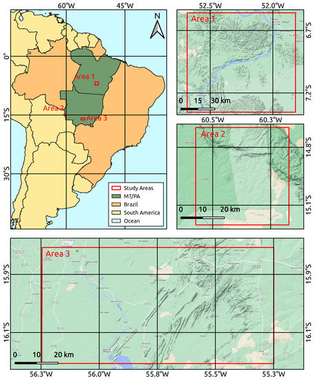
Figure 2.
Study area locations.
Concerning Areas 1, 2 and 3, we took images obtained by the OLI (30 m spatial resolution of size pixels wide), MSI (10 m, pixels wide), and MODIS (500 m, pixels wide) sensors onboard the Landsat-8, Sentinel-2, and Terra satellites, respectively. The green, red, NIR, and SWIR wavelength bands were also used in order to properly run the analysis methods. Knowing the tendency of fire incidence in these regions, all images available from 1 August to 31 October 2020, limited to 50% cloud/shadow coverage over the study area, were considered in the analyses. Table 2 presents the dates of the images that meet these criteria.
Table 2.
Dates of the images considered in the experiments.
Regarding the reference image (i.e., , Section 3) required by the UFD+MRF method, we adopted the median image from all images acquired by the respective sensors between 1 June 2019 and 30 June 2020. A total of 9, 36, and 49 images were found in the considered period to compute the reference images for Areas 1, 2, and 3, respectively. Figure 3, Figure 4 and Figure 5 illustrate images of the study areas according to the reference image and the later instant.
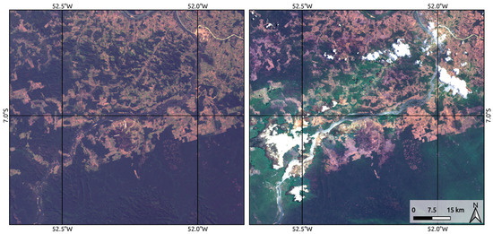
Figure 3.
Reference image (left) and the later instant (right—14 September 2020) for Area 1. Representations in natural color composition.
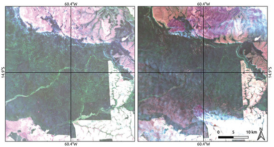
Figure 4.
Reference image (left) and the later instant (right—9 October 2020) for Area 2. Representations in natural color composition.
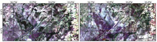
Figure 5.
Reference image (left) and the later instant (right—15 October 2020) for Area 3. Representations in natural color composition.
Aiming at quantifying the accuracies of the methods when they are applied for mapping the burned areas over the study areas and period of analysis, the locations of fire events registered between 1 August and 31 October 2020 in the DBFires database [60] were taken as a benchmark for burned areas. Similarly, a 1 km-spaced point-wise grid covering regions not affected by fire was taken as ground-truth for non-burned areas. Figure 6 depicts the above-mentioned benchmark dataset.
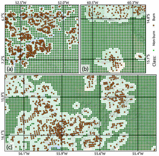
Figure 6.
Ground-truth samples for (a) Area 1, (b) Area 2, and (c) Area 3. Point-wise burning occurrences recorded from 1 August to 31 October 2020 [60].
As a reference for qualitative comparisons, we obtained estimates from “MCD64A1 MODIS Burned Area Monthly” [67] (500 m of spatial resolution), herein referred to as the MODIS Burned Areas (MBA) product.
Based on this product, positions/pixels in the study areas where the indication of fire shows confidence superior to 90% are taken as a “burn”; otherwise, they are considered “non-burn”. Despite the broad difference of spatial resolution between the MBA product and the OLI and MSI images, it should be stressed that this product allows for verifying the agreement between the mappings generated by the analyzed methods and the expected results. Consequently, the qualitative assessments are limited to verifying if the frequencies and spatial distribution of mapped burned areas are compatible with the expectations.
4.3. Results
Prior to applying the MTDNBR, GKM, and UFD+MRF methods, Figure 7, Figure 8 and Figure 9 show the behavior of the NBR index concerning the reference images at selected instants in each study area for data inspection purposes. With respect to Area 1 (Figure 7), it is possible to notice that, in comparison to the reference image, changes in NBR values occur progressively from August to October. In Area 2 (Figure 8), the most significant changes are only highlighted at the last instant (i.e., 9 October 2020). Conversely, the most relevant changes in Area 3 (Figure 9) occur in September and October.
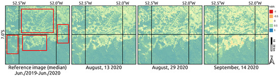
Figure 7.
The NBR behavior for the reference image and individual instants regarding Area 1. Regions delimited by red rectangles highlight places with potential changes over time.
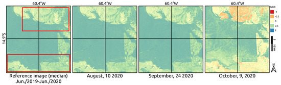
Figure 8.
The NBR behavior for the reference image and individual instants regarding Area 2. Regions delimited by red rectangles highlight places with potential changes over time.
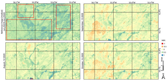
Figure 9.
The NBR behavior for the reference image and individual instants regarding Area 3. Regions delimited by red rectangles highlight places with potential changes over time.
Considering the evaluated study areas (Figure 2) and their corresponding sensors, all examined methods were applied to map the burned regions over the period of analysis (1 August to 31 October 2020—Table 2). The obtained results were quantitatively assessed in terms of OA, F1-score, MCC, and kappa coefficient by using the ground-truth reference dataset of burned and non-burned locations (Figure 6). Table 3 lists the computed accuracy values. The resulting burned area maps for each study area are presented in Figure 10, Figure 11 and Figure 12 and discussed in Section 4.4.
Table 3.
Accuracy values summary.
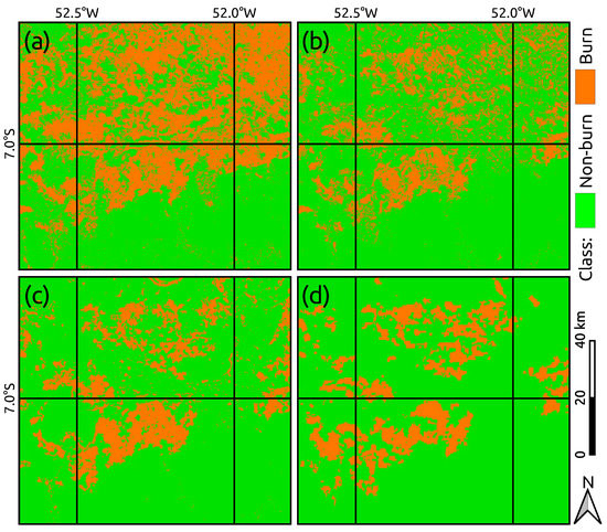
Figure 10.
The mapping of fire-affected locations provided by the (a) MTDNBR, (b) GKM, and (c) UFD+MRF methods for Area 1 using OLI data. Estimates from the MBA product are shown in (d). Representations comprise the analyzed period of 1 August to 31 October 2020.
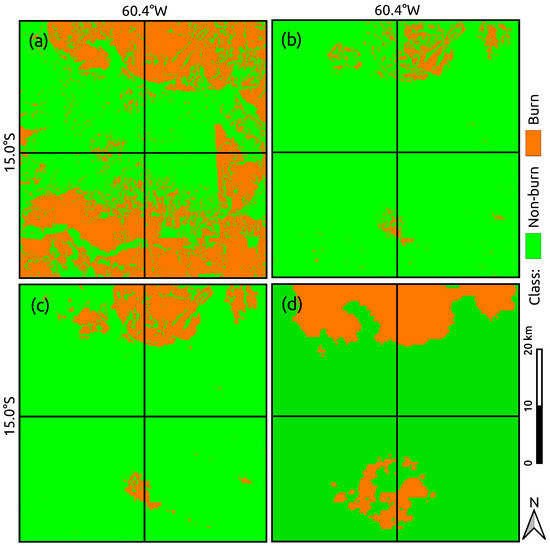
Figure 11.
The mapping of fire-affected locations provided by the (a) MTDNBR, (b) GKM, and (c) UFD+MRF methods for Area 2 using MSI data. Estimates from the MBA product are shown in (d). Representations comprise the analyzed period of 1 August to 31 October 2020.
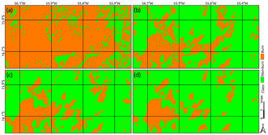
Figure 12.
The mapping of fire-affected locations provided by the (a) MTDNBR, (b) GKM, and (c) UFD+MRF methods for Area 3 using MODIS data. Estimates from the MBA product are shown in (d).
Regardless of the study area/adopted sensor, one can notice that the proposed methodology achieved better accuracy values in comparison to other state-of-the-art methods. While low accuracy values were assigned to the MTDNB method, more competitive performance was demonstrated by the GKM framework concerning Areas 1 and 3.
The run times for each examined method and study area are also included in Table 3. The ability to handle noisy data efficiently combined with the high-accuracy results produced by the proposed approach come with the price of computing the parameters of the Logit model, obtained by the descending gradient scheme, and the application of the ICM algorithm. Since the MTDNBR and GKM approaches only comprise thresholding-based operations, the assigned computational times for both methods are also compatible. The present UFD+MRF methodology took about 180 s, 66 s, and 10 s to processes the data sets for Areas 1, 2, and 3, respectively. Nonetheless, such a computational cost is relieved by more regular and behaved (i.e., less noisy) mappings, as shown in Figure 10, Figure 11 and Figure 12 and discussed in Section 4.4.
4.4. Discussion
Concerning the obtained results for Area 1 with OLI data, the MTDBNR method (Figure 10a) provides a map that is highly prone to false-positive labeling of burned areas in comparison to the GKM and UFD+MRF methods (Figure 10b,c). Conversely, the GKM and UFD+MRF methods deliver better discrimination between burned and non-burned areas. However, one can verify that our methodology outputs a more consistent and well-behaved mapping (i.e., less isolated pixels) in contrast to the GKM method. In terms of qualitative analysis, despite the distinct spatial resolution differences, the visual adherence of the mapping produced by the proposed approach over existing methods is evident when compared with the MBA product (Figure 10d).
Similar behavior can be observed concerning the qualitative analysis for Area 2, where 10 m spatial resolution data is used. The MTDNBR method is evidently assigned to frequent false-burn detection (Figure 11a). By inspecting the results from the GKM framework (Figure 11b) together with the ground-truth data from the MBA product (Figure 11d), one can find that the achieved mapping was unable to properly capture the burned segments. In contrast, our UFD+MRF approach (Figure 11c) delivers a fire mapping closer to the reference data.
Finally, focusing our inspections on the third study area, by using MODIS data with a spatial resolution (500 m) compatible with the reference MBA product (Figure 12d), the analyzed methods perform similarly to the previous study areas. While the MTDBNR method tends to overestimate the burning occurrences, the GKM method has frequent isolated regions/pixels (noisy aspect). Again, the output produced by the UFD+MRF approach (Figure 12c) is visually more adherent to the MBA product (Figure 12d).
It is worth stressing that the identified burned areas occurred in distinct instants of the analyzed period, as previously shown in Figure 7, Figure 8 and Figure 9. Hence, our proposal’s capability for dealing with multitemporal data in an accurate manner is also evident.
According to the obtained maps for Area 1, small burned areas were identified by the proposed approach (e.g., near coordinates 52.5W/6.7S or 65.2W/6.9S—Figure 10c) that also match the references made available in the DBFires database (Figure 6a). However, one may notice that these specific segments were not properly detected when checking the MBA product. One plausible reason behind this behavior is the different data resolutions used in each mapping (i.e., UFD+MRF/OLI—30 m; MBA/MODIS—500 m).
Similarly, regarding the burned area map obtained for Area 2, the input data spatial resolution (i.e., MS—10 m) leads to a consistent result in identifying isolated regions affected by fires (e.g., near 60.3W/15.1S and 60.5W/14.8S—Figure 11c). Indeed, these burned regions are confirmed by inspecting the DBFires reference samples (Figure 6b). On the other hand, the estimates from the MBA product indicate the fire incidence over the entire upper portion of the study area (Figure 11d), thus contradicting the DBFires records as well as the NBR variations over the evaluation period (Figure 8). Considering the accuracies in Table 3 and the above-discussed points, our approach can generate accurate burned-area estimates with better spatial resolution compared to the outputs generated by the MBA product.
Lastly, when using MODIS images as input data, the current methodology presents both similarities and differences compared to the MBA product for Area 3. For example, by taking as reference the reported locations in DBFire (Figure 6c), the lower-left (i.e., below coordinate 56.1W; 16.1S) and center-right (between coordinate 55.6–55.4W/15.9–16.0S) regions differ from the mapping produced by the MBA product. The same is not observed in the burned area mapping provided by the UFD+MRF method. A possible reason for such divergence, which also explains a few differences already discussed for Areas 1 and 2, comes from the minimum confidence level (90%) considered for the MBA product to detect burned areas. At the cost of increased inclusion errors and negative impacts on the representation consistency, identifying such regions through the MBA product can be achieved using lower confidence levels.
Both the quantitative and qualitative inspections presented above corroborate the scores outlined in Figure 13, where the proportions of true and false positives (burned areas) and negatives (non-burned areas) were computed from the ground-truth reference sets (Figure 6). The computed values reinforce that the proposed methodology is subject to inferior wrong decision proportions (i.e., false positive and negative errors) when compared against MTDNBR and GKM methods.
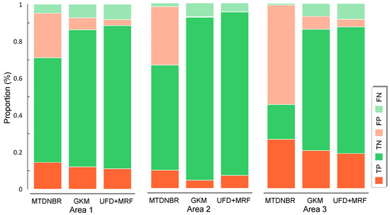
Figure 13.
True/false positive/negative detection proportions.
From the analyzed results, the proposed methodology turns out to be effective when mapping burning areas independently of the adopted multispectral sensors. Considering the operational utilization and the ground-truth data taken from the well-known MBA product, our data-driven approach ca be successfully used to generate mappings with higher spatial resolution. On the other hand, the resulting temporal estimates will also depend on the adopted sensor’s revisiting rate and cloud/shadow cover condition. However, when the main application interest lies in identifying burned areas in a given period of interest, the proposed methodology becomes more suitable.
Another aspect to observe when using our UFD+MRF approach is that it may be considered a ready-to-use core component of a monitoring system, designed to detect and quantify new burned areas as it is updated by newly acquired images. Finally, by using other spectral indices in a delta-type scheme (e.g., NDVI and NDWI [68,69]), the architecture described in this paper (Figure 1) can be easily customized for other application domains, as for example, deforestation and flooding mapping.
5. Conclusions
We proposed an unsupervised approach for identifying burned areas with multitemporal remote-sensing data. Spectral indices, logistic regression, and Markov random field modeling are the main concepts that support this proposal. The central idea lies in measuring the progressive deviations over time from a fixed reference image and then modeling these deviations as a probability function to map locations affected by fire in some instant of the time series. Three study cases, considering distinct regions and remote sensors, were carried out to assess the proposed method. Comparisons with two approaches found in the literature were included in the experiments.
The results showed a high adherence between the proposed method and a ground-truth reference data set. Qualitative comparisons with a coarse resolution product derived from the MODIS sensor for fire mapping purposes were also included in the analysis. While one concurrent method was unable to deliver consistent results, the other provided less regularized (noisy) mappings.
The proposed method’s robustness comes from a deviation measure computed over time, which is submitted to a probabilistic treatment to include the contextual information. On the other hand, the concurrent method (MTDNBR), as an alternative to mapping burned areas in temporal series with basis in the , is highly subject to errors due to the use of fixed thresholds, as well as by the targets’ spectral variation over time.
Although the proposed method demonstrates greater computational run-time when compared to the simple threshold-based competitor, it is worth highlighting that it still comprises a light-cost algorithm.
In summary, we state as main contributions of this paper:
- A fully unsupervised learning formulation for discriminating and mapping burned areas using multispectral image time series;
- A conceptual formalization that can be conveniently customized for other remote sensing applications in addition to mapping fire-impacted areas;
- A comprehensive set of experiments and descriptive analyses using distinct sensors followed by quantitative and qualitative comparisons with existing methods from the specialized literature, thus advancing the field.
In future work, we plan to: (i) adapt and investigate the use of the proposed framework on other environmental issues, such as deforestation, flooding, oil spills, glaciers melting, etc.; (ii) analyze other probability modeling approaches (e.g., [70]); (iii) include a confidence measure concerning the resulting mappings; (iv) extend the proposed method beyond binary outputs; (v) adapt the proposed method to operate with radar images.
Author Contributions
Conceptualization—R.G.N., A.E.O.L., A.C.F. and W.C.; funding acquisition—R.G.N. and W.C.; investigation—R.G.N., A.E.O.L., A.C.F. and W.C.; methodology—R.G.N., A.E.O.L., A.C.F. and W.C.; validation—R.G.N., A.E.O.L., A.C.F. and W.C.; writing original draft—R.G.N. and A.E.O.L. All authors have read and agreed to the published version of the manuscript.
Funding
This research was funded by the São Paulo Research Foundation (FAPESP), grants 2021/01305-6 and 2021/03328-3, and the National Council for Scientific and Technological Development (CNPq), grant 316228/2021-4. The APC was partially funded by São Paulo State University (UNESP).
Data Availability Statement
The code of framework proposed in Section 3 is freely available at https://github.com/rogerionegri/ufd (accessed on 20 October 2022).
Conflicts of Interest
The authors declare no conflict of interest. The funders had no role in the design of the study; in the collection, analyses, or interpretation of data; in the writing of the manuscript, or in the decision to publish the results.
Abbreviations
The following abbreviations are used in this manuscript:
| RS | Remote Sensing |
| MODIS | Moderate-Resolution Imaging Spectroradiometer |
| OLI | Operational Land Imager |
| MSI | Multispectral Instrument |
| NDVI | Normalized Difference Vegetation Index |
| NBR | Normalized Burn Ratio |
| BAIS | Burned Area Index for Sentinel |
| NBR | Difference Normalized Burn Ratio |
| RNBR | Relative NBR |
| NDWI | Normalized Difference Water Index |
| SAVI | Soil Adjusted Vegetation Index |
| VIS | Visible Wavelength |
| NIR | Near-Infrared Wavelength |
| SWIR | Shortwave-infrared |
| ICM | Iterated Conditional Modes |
| MRF | Markov Random Field |
| UFD | Unsupervised Fire Detection |
| API-GEE | Application Programming Interface for Google Earth Engine |
| IDL | Interactive Data Language |
| MTDNBR | Multi-Temporal NBR |
| GKM | Gholinejad–Khesali’s Method |
| MBA | MODIS Burned Area |
| TP/FP | True/False Positive |
| TN/FN | True/False Negative |
| MCC | Matthews Correlation Coefficient |
| OA | Overall Accuracy |
References
- Luterbacher, J.; Paterson, L.; von Borries, R.; Solazzo, K.; Devillier, R.; Castonguay, S. United in Science 2021: A Multi-Organization High-Level Compilation of the Latest Climate Science Information; Technical Report; Partner Organizations: World Meteorological Organization (WMO), Global Carbon Project (GCP), Intergovernmental Panel on Climate Change (IPCC), United Nations Environment Programme (UNEP), World Health Organization (WHO), the Met Office (United Kingdom, UK); World Meteorological Organization (WMO): Geneva, Switzerland, 2021. [Google Scholar]
- Stott, P.A.; Christidis, N.; Otto, F.E.; Sun, Y.; Vanderlinden, J.P.; van Oldenborgh, G.J.; Vautard, R.; von Storch, H.; Walton, P.; Yiou, P. Attribution of extreme weather and climate-related events. Wiley Interdiscip. Rev. Clim. Chang. 2016, 7, 23–41. [Google Scholar] [CrossRef]
- Van Aalst, M.K. The impacts of climate change on the risk of natural disasters. Disasters 2006, 30, 5–18. [Google Scholar] [CrossRef]
- AghaKouchak, A. A multivariate approach for persistence-based drought prediction: Application to the 2010–2011 East Africa drought. J. Hydrol. 2015, 526, 127–135. [Google Scholar] [CrossRef]
- Rajsekhar, D.; Singh, V.P.; Mishra, A.K. Multivariate drought index: An information theory based approach for integrated drought assessment. J. Hydrol. 2015, 526, 164–182. [Google Scholar] [CrossRef]
- Da Silva, S.S.; Fearnside, P.M.; de Alencastro Graça, P.M.L.; Brown, I.F.; Alencar, A.; de Melo, A.W.F. Dynamics of forest fires in the southwestern Amazon. For. Ecol. Manag. 2018, 424, 312–322. [Google Scholar] [CrossRef]
- Motazeh, A.G.; Ashtiani, E.F.; Baniasadi, R.; Choobar, F.M. Rating and mapping fire hazard in the hardwood Hyrcanian forests using GIS and expert choice software. For. Ideas 2013, 19, 141–150. [Google Scholar]
- Prestes, N.C.C.S.; Massi, K.G.; Silva, E.A.; Nogueira, D.S.; de Oliveira, E.A.; Freitag, R.; Marimon, B.S.; Marimon-Junior, B.H.; Keller, M.; Feldpausch, T.R. Fire effects on understory forest regeneration in southern Amazonia. Front. For. Glob. Chang. 2020, 3, 10. [Google Scholar] [CrossRef]
- Filipponi, F. BAIS2: Burned Area Index for Sentinel-2. Proceedings 2018, 2, 364. [Google Scholar] [CrossRef]
- Lasaponara, R.; Proto, A.M.; Aromando, A.; Cardettini, G.; Varela, V.; Danese, M. On the Mapping of Burned Areas and Burn Severity Using Self Organizing Map and Sentinel-2 Data. IEEE Geosci. Remote Sens. Lett. 2020, 17, 854–858. [Google Scholar] [CrossRef]
- Pereira, A.A.; Pereira, J.; Libonati, R.; Oom, D.; Setzer, A.W.; Morelli, F.; Machado-Silva, F.; De Carvalho, L.M.T. Burned area mapping in the Brazilian Savanna using a one-class support vector machine trained by active fires. Remote Sens. 2017, 9, 1161. [Google Scholar] [CrossRef]
- Yuan, Q.; Shen, H.; Li, T.; Li, Z.; Li, S.; Jiang, Y.; Xu, H.; Tan, W.; Yang, Q.; Wang, J.; et al. Deep learning in environmental remote sensing: Achievements and challenges. Remote Sens. Environ. 2020, 241, 111716. [Google Scholar] [CrossRef]
- Martínez-Álvarez, F.; Tien Bui, D. Advanced Machine Learning and Big Data Analytics in Remote Sensing for Natural Hazards Management. Remote Sens. 2020, 12, 301. [Google Scholar] [CrossRef]
- Alonso-Canas, I.; Chuvieco, E. Global burned area mapping from ENVISAT-MERIS and MODIS active fire data. Remote Sens. Environ. 2015, 163, 140–152. [Google Scholar] [CrossRef]
- Giglio, L.; Loboda, T.; Roy, D.P.; Quayle, B.; Justice, C.O. An active-fire based burned area mapping algorithm for the MODIS sensor. Remote Sens. Environ. 2009, 113, 408–420. [Google Scholar] [CrossRef]
- Birch, D.S.; Morgan, P.; Kolden, C.A.; Abatzoglou, J.T.; Dillon, G.K.; Hudak, A.T.; Smith, A.M. Vegetation, topography and daily weather influenced burn severity in central Idaho and western Montana forests. Ecosphere 2015, 6, 1–23. [Google Scholar] [CrossRef]
- Gibson, R.; Danaher, T.; Hehir, W.; Collins, L. A remote sensing approach to mapping fire severity in south-eastern Australia using sentinel 2 and random forest. Remote Sens. Environ. 2020, 240, 111702. [Google Scholar] [CrossRef]
- Mohajane, M.; Costache, R.; Karimi, F.; Bao Pham, Q.; Essahlaoui, A.; Nguyen, H.; Laneve, G.; Oudija, F. Application of remote sensing and machine learning algorithms for forest fire mapping in a Mediterranean area. Ecol. Indic. 2021, 129, 107869. [Google Scholar] [CrossRef]
- Tien Bui, D.; Le, K.T.T.; Nguyen, V.C.; Le, H.D.; Revhaug, I. Tropical Forest Fire Susceptibility Mapping at the Cat Ba National Park Area, Hai Phong City, Vietnam, Using GIS-Based Kernel Logistic Regression. Remote Sens. 2016, 8, 347. [Google Scholar] [CrossRef]
- Collins, L.; McCarthy, G.; Mellor, A.; Newell, G.; Smith, L. Training data requirements for fire severity mapping using Landsat imagery and random forest. Remote Sens. Environ. 2020, 245, 111839. [Google Scholar] [CrossRef]
- Pacheco, A.d.P.; Junior, J.A.d.S.; Ruiz-Armenteros, A.M.; Henriques, R.F.F. Assessment of k-Nearest Neighbor and Random Forest Classifiers for Mapping Forest Fire Areas in Central Portugal Using Landsat-8, Sentinel-2, and Terra Imagery. Remote Sens. 2021, 13, 1345. [Google Scholar] [CrossRef]
- Mallinis, G.; Mitsopoulos, I.; Chrysafi, I. Evaluating and comparing Sentinel 2A and Landsat-8 Operational Land Imager (OLI) spectral indices for estimating fire severity in a Mediterranean pine ecosystem of Greece. GISci. Remote Sens. 2018, 55, 1–18. [Google Scholar] [CrossRef]
- Key, C.; Benson, N. Landscape Assessment: Ground Measure of Severity, the Composite Burn Index; and Remote Sensing of Severity, the Normalized Burn Ratio; Technical Report RMRS-GTR-164-CD: LA 1-51; USDA Forest Service: Washington, DC, USA; Rocky Mountain Research Station: Ogden, UT, USA; USGS Publications Warehouse: Virgina, VA, USA, 2006.
- Miller, J.D.; Thode, A.E. Quantifying burn severity in a heterogeneous landscape with a relative version of the delta Normalized Burn Ratio (dNBR). Remote Sens. Environ. 2007, 109, 66–80. [Google Scholar] [CrossRef]
- Cai, L.; Wang, M. Is the RdNBR a better estimator of wildfire burn severity than the dNBR? A discussion and case study in southeast China. Geocarto Int. 2022, 37, 758–772. [Google Scholar] [CrossRef]
- Gholinejad, S.; Khesali, E. An automatic procedure for generating burn severity maps from the satellite images-derived spectral indices. Int. J. Digit. Earth 2021, 14, 1659–1673. [Google Scholar] [CrossRef]
- McKenna, P.; Erskine, P.D.; Lechner, A.M.; Phinn, S. Measuring fire severity using UAV imagery in semi-arid central Queensland, Australia. Int. J. Remote Sens. 2017, 38, 4244–4264. [Google Scholar] [CrossRef]
- Hu, X.; Ban, Y.; Nascetti, A. Uni-Temporal Multispectral Imagery for Burned Area Mapping with Deep Learning. Remote Sens. 2021, 13, 1509. [Google Scholar] [CrossRef]
- Ba, R.; Song, W.; Li, X.; Xie, Z.; Lo, S. Integration of Multiple Spectral Indices and a Neural Network for Burned Area Mapping Based on MODIS Data. Remote Sens. 2019, 11, 326. [Google Scholar] [CrossRef]
- Ban, Y.; Zhang, P.; Nascetti, A.; Bevington, A.R.; Wulder, M.A. Near real-time wildfire progression monitoring with Sentinel-1 SAR time series and deep learning. Sci. Rep. 2020, 10, 1322. [Google Scholar] [CrossRef]
- Matricardi, E.A.; Skole, D.L.; Pedlowski, M.A.; Chomentowski, W. Assessment of forest disturbances by selective logging and forest fires in the Brazilian Amazon using Landsat data. Int. J. Remote Sens. 2013, 34, 1057–1086. [Google Scholar] [CrossRef]
- Barmpoutis, P.; Papaioannou, P.; Dimitropoulos, K.; Grammalidis, N. Comparisons of Diverse Machine Learning Approaches for Wildfire Susceptibility Mapping. Symmetry 2020, 12, 604. [Google Scholar]
- Coca, M.; Datcu, M. Anomaly Detection in Post Fire Assessment. In Proceedings of the IEEE International Geoscience and Remote Sensing Symposium (IGARSS), Brussels, Belgium, 11–16 July 2021; pp. 8620–8623. [Google Scholar]
- Vivone, G.; Dalla Mura, M.; Garzelli, A.; Pacifici, F. A Benchmarking Protocol for Pansharpening: Dataset, Preprocessing, and Quality Assessment. IEEE J. Sel. Top. Appl. Earth Obs. Remote Sens. 2021, 14, 6102–6118. [Google Scholar] [CrossRef]
- Luz, A.E.O.; Negri, R.G.; Massi, K.G.; Colnago, M.; Silva, E.A.; Casaca, W. Mapping Fire Susceptibility in the Brazilian Amazon Forests Using Multitemporal Remote Sensing and Time-Varying Unsupervised Anomaly Detection. Remote Sens. 2022, 14, 2429. [Google Scholar] [CrossRef]
- Wang, P.; Wang, L.; Leung, H.; Zhang, G. Super-Resolution Mapping Based on Spatial–Spectral Correlation for Spectral Imagery. IEEE Trans. Geosci. Remote Sens. 2021, 59, 2256–2268. [Google Scholar] [CrossRef]
- Khosravi, K.; Panahi, M.; Tien Bui, D. Spatial prediction of groundwater spring potential mapping based on an adaptive neuro-fuzzy inference system and metaheuristic optimization. Hydrol. Earth Syst. Sci. 2018, 22, 4771–4792. [Google Scholar] [CrossRef]
- Verstraete, M.M.; Pinty, B. Designing optimal spectral indexes for remote sensing applications. IEEE Trans. Geosci. Remote Sens. 1996, 34, 1254–1265. [Google Scholar] [CrossRef]
- Xue, J.; Su, B. Significant remote sensing vegetation indices: A review of developments and applications. J. Sens. 2017, 2017, 1353691. [Google Scholar] [CrossRef]
- Rouse, J.W.; Haas, R.H.; Schell, J.A.; Deering, D.W. Monitoring vegetation systems in the Great Plains with ERTS. In Third Earth Resources Technology Satellite-1 Symposium; NASA Special Publication 351; NASA: Washington, DC, USA, 1974; Volume 1. [Google Scholar]
- Gao, B. NDWI—A normalized difference water index for remote sensing of vegetation liquid water from space. Remote Sens. Environ. 1996, 58, 257–266. [Google Scholar] [CrossRef]
- Huete, A.R. A soil-adjusted vegetation index (SAVI). Remote Sens. Environ. 1988, 25, 295–309. [Google Scholar] [CrossRef]
- Sobrino, J.A.; Llorens, R.; Fernández, C.; Fernández-Alonso, J.M.; Vega, J.A. Relationship between soil burn severity in forest fires measured in situ and through spectral indices of remote detection. Forests 2019, 10, 457. [Google Scholar] [CrossRef]
- Veraverbeke, S.; Dennison, P.; Gitas, I.; Hulley, G.; Kalashnikova, O.; Katagis, T.; Kuai, L.; Meng, R.; Roberts, D.; Stavros, N. Hyperspectral remote sensing of fire: State-of-the-art and future perspectives. Remote Sens. Environ. 2018, 216, 105–121. [Google Scholar] [CrossRef]
- Hosmer, D.; Lemeshow, S.; Sturdivant, R. Applied Logistic Regression; Wiley Series in Probability and Statistics; Wiley: New York, NY, USA, 2013. [Google Scholar]
- McCullagh, P.; Nelder, J.A. Generalized Linear Models, 2nd ed.; Chapmann and Hall: New York, NY, USA, 1989. [Google Scholar]
- Berk, R.A. Statistical Learning from a Regression Perspective, 2nd ed.; Springer Texts in Statistics; Springer: Cham, Switzerland, 2016. [Google Scholar]
- Kochenderfer, M.; Wheeler, T. Algorithms for Optimization; MIT Press: Cambridge, MA, USA, 2019. [Google Scholar]
- Besag, J. On the statistical analysis of dirty pictures. J. R. Stat. Soc. Ser. B (Methodol.) 1986, 48, 259–302. [Google Scholar] [CrossRef]
- Frery, A.C.; Correia, A.H.; Freitas, C.C. Classifying Multifrequency Fully Polarimetric Imagery with Multiple Sources of Statistical Evidence and Contextual Information. IEEE Trans. Geosci. Remote Sens. 2007, 45, 3098–3109. [Google Scholar] [CrossRef]
- Géron, A. Hands-On Machine Learning with Scikit-Learn and TensorFlow: Concepts, Tools, and Techniques to Build Intelligent Systems; O’Reilly Media: Sebastopol, CA, USA, 2017. [Google Scholar]
- Van Rossum, G.; Drake, F.L. The Python Language Reference Manual; Network Theory Ltd.: Godalming, UK, 2011. [Google Scholar]
- Gorelick, N.; Hancher, M.; Dixon, M.; Ilyushchenko, S.; Thau, D.; Moore, R. Google Earth Engine: Planetary-scale geospatial analysis for everyone. Remote Sens. Environ. 2017, 202, 18–27. [Google Scholar] [CrossRef]
- McKinney, W. Data structures for statistical computing in Python. In Proceedings of the 9th Python in Science Conference, Austin, TX, USA, 28 June–3 July 2010; Volume 445, pp. 51–56. [Google Scholar]
- Westra, E. Python Geospatial Development; Packt Publishing: Birmingham, UK, 2010. [Google Scholar]
- Gómez-Chova, L.; Amorós-López, J.; Mateo-García, G.; Muñoz-Marí, J.; Camps-Valls, G. Cloud masking and removal in remote sensing image time series. J. Appl. Remote Sens. 2017, 11, 015005. [Google Scholar] [CrossRef]
- Basso, D.; Colnago, M.; Azevedo, S.; Silva, E.; Pina, P.; Casaca, W. Combining morphological filtering, anisotropic diffusion and block-based data replication for automatically detecting and recovering unscanned gaps in remote sensing images. Earth Sci. Inform. 2021, 14. [Google Scholar] [CrossRef]
- Exelis. IDL—Interactive Data Language; Version 8.8; Exelis Visual Information Solutions: Boulder, CO, USA, 2021. [Google Scholar]
- United Nations. United Nations—Normalized Burn Ratio (NBR); United Nations: New York, NY, USA, 2022. [Google Scholar]
- INPE. BDQueimadas: A Real-Time Burning Forest Database; Instituto Nacional de Pesquisas Espaciais: São José dos Campos, Brazil, 2022.
- Setzer, A.W.; Sismanoglu, R.A.; dos Santos, J.G.M. Método do Cálculo do Risco de Fogo do Programa do INPE—Versão 11.Junho/2019; Technical Report; National Institute for Space Research: São José dos Campos, Brazil, 2019. [Google Scholar]
- Story, M.; Congalton, R.G. Accuracy assessment: A user’s perspective. Photogramm. Eng. Remote Sens. 1986, 52, 397–399. [Google Scholar]
- Rijsbergen, C.J.V. Information Retrieval, 2nd ed.; Butterworth-Heinemann: Oxford, UK, 1979. [Google Scholar]
- Congalton, R.G.; Green, K. Assessing the Accuracy of Remotely Sensed Data: Principles and Practices, 3rd ed.; CRC Press: Boca Raton, FL, USA, 2019. [Google Scholar]
- Negri, R.G.; Frery, A.C.; Casaca, W.; Azevedo, S.; Dias, M.A.; Silva, E.A.; Alcântara, E.H. Spectral–Spatial-Aware Unsupervised Change Detection With Stochastic Distances and Support Vector Machines. IEEE Trans. Geosci. Remote Sens. 2021, 59, 2863–2876. [Google Scholar] [CrossRef]
- Matthews, B.W. Comparison of the predicted and observed secondary structure of T4 phage lysozyme. Biochim. Biophys. Acta—Protein Struct. 1975, 405, 442–451. [Google Scholar] [CrossRef]
- Giglio, L.; Boschetti, L.; Roy, D.; Hoffmann, A.A.; Humber, M.; Hall, J.V. Collection 6 MODIS Burned Area Product User’s Guide (Version 1.3); National Aeronautics and Space Administration: Washinton, DC, USA, 2020.
- Tran, B.N.; Tanase, M.A.; Bennett, L.T.; Aponte, C. Evaluation of Spectral Indices for Assessing Fire Severity in Australian Temperate Forests. Remote Sens. 2018, 10, 1680. [Google Scholar] [CrossRef]
- Thuan, C.; Xulin, G.; Kazuo, T. Temporal dependence of burn severity assessment in Siberian larch (Larix sibirica) forest of northern Mongolia using remotely sensed data. Int. J. Wildland Fire 2016, 25, 685–698. [Google Scholar] [CrossRef]
- Casaca, W.; Gois, J.P.; Batagelo, H.C.; Taubin, G.; Nonato, L.G. Laplacian Coordinates: Theory and Methods for Seeded Image Segmentation. IEEE Trans. Pattern Anal. Mach. Intell. 2021, 43, 2665–2681. [Google Scholar] [CrossRef] [PubMed]


Publisher’s Note: MDPI stays neutral with regard to jurisdictional claims in published maps and institutional affiliations. |
© 2022 by the authors. Licensee MDPI, Basel, Switzerland. This article is an open access article distributed under the terms and conditions of the Creative Commons Attribution (CC BY) license (https://creativecommons.org/licenses/by/4.0/).