A Novel Hybrid LMD–ETS–TCN Approach for Predicting Landslide Displacement Based on GPS Time Series Analysis

Abstract

Landslide disasters cause serious property losses and casualties every year. Landslide displacement prediction is fundamental for mitigating landslide disasters. Several approaches have been used to predict landslide displacement, yet a more accurate and reliable displacement prediction still has a poor understanding of landslide early warning systems for landslide mitigation, due to limited data and mutational displacements. To boost the robustness and accuracy of landslide displacement prediction, this paper assembled a new hybrid model containing the local mean decomposition (LMD), innovations state space models for exponential smoothing (ETS), and the temporal convolutional network (TCN). The proposed model, which is based on over 10 years of long-term time series monitoring GPS data, was tested on the selected case—stepwise Baijiabao landslide in the Three Gorges Reservoir area of China (TGRA) was tested by the proposed model. The results presented that the LMD–ETS–TCN model has the best performance in comparison with other benchmark models. Compared with autoregressive integrated moving average (ARIMA), support vector regression (SVR), and long short-term memory neural network (LSTM), the accuracy was noticeably improved by an average of 40.9%, 46.2%, and 22.1%, respectively. The robustness and effectiveness of the presented approach are attested, and it has discernible improvements for landslide displacement prediction.

1. Introduction

Landslides are frequent but dangerous geological disasters that threaten people’s safety and property losses [1,2,3,4,5]. Numerous new landslides have happened because of the initial impoundment of the Three Gorges Reservoir Area (TGRA) in June 2003 [6,7], while numerous ancient landslides have shown signs of revival deformation [8,9]. Hence, to analyze the mechanism of landslide evolution and to reduce the casualties caused by landslides, early warning and long-term monitoring systems (EWLS) are set up in many landslides in the TGRA [10,11,12]. Landslide displacement prediction (LDP) using monitoring data is quite important for EWLS, providing alert information for decision-makers and reducing the harm caused by landslides [13,14]. Thus, accurate and reliable landslide displacement prediction is a useful approach to lessen landslide hazards.

Several approaches are used for predicting landslide displacement, mainly including physically based and data-driven methods. Landslide displacement prediction can be traced back to the three stages of the step-like landslide creep theory proposed by Saito in the 1960s [15]. According to the creep theory and other physical models of soil and rock masses, some deterministic models have been tested [16], such as the Saito model [15,17] and the Voight model [18]. The characteristics of these models are that they have obvious physical mechanisms but have severe limitations of application and rely on the experience of experts. Because models simplify geological and mechanical mechanisms, models may not accord with facts. With the development of statistics, many statistical approaches have been used to predict landslide displacement, such as the Verhulst model [19] and the gray system model [20]. Most of these models are nonlinear models without certain support by geological and mechanical mechanisms. In the past decade, with the rapid development of artificial intelligence (AI), various studies have been devoted to applying AI models to predicting landslide displacement. For example, Du et al. [21] trained a backpropagation neural network (BPNN) model with chosen landslide-inducing factors to predict displacement in two colluvial landslides. Huang et al. [22] utilized an extreme learning machine (ELM) to forecast landslide displacement. Cai et al. [23] presented a least-squares support vector machine (LSSVM) with a genetic algorithm (GA) for predicting landslide displacement. However, these neural network models are fully connected, and there may be producing information leakage during training, which leads to overfitting of the training sets. To solve the mentioned issue, a kind of deep learning (DL) named the recurrent neural network (RNN), whose architecture was designed for series data, was applied to landslide displacement prediction [24]. RNN and its improved models, including long short-term memory (LSTM) neural networks and gated recurrent unit (GRU), have been extensively used in landslide displacement prediction [25,26,27,28]. DL has exhibited superior operation over conventional machine-learning methods and has proven to be a promising tool for landslide prediction [29,30,31].

Landslide cumulative displacement refers to geological conditions, hydrological environment, precipitation, and other external inducing factors. Cumulative displacement decomposition is an additive decomposition that is divided into two parts: trend displacement and periodic displacement, respectively [32,33]. The trend displacement determined by geological conditions showed a long-term increase in the landslide. Periodic displacement relies on external factors, such as reservoir level and precipitation [21]. Decomposing cumulative displacement is beneficial to reduce the difficulty of prediction. Moving average, empirical mode decomposition (EMD), and modified EMD models, which include ensemble empirical mode decomposition and complementary ensemble empirical mode decomposition are regular methods to decompose landslide displacement [34,35,36,37]. The moving average lags behind the latest datum by half the sample width [38]. By EMD and modified EMDs, the upper envelope and lower envelope of the original signal are obtained by cubic spline interpolation for all extremum points, respectively, which easily forms an over-envelope or under-envelope. Polynomial fitting is often used for trend term prediction, but polynomial fitting does not perform well for long-term series [39,40], which need to be split into several parts [26]. The architecture of RNN has a major problem of exploding or vanishing gradients, which has led to the progress of LSTM and GRU, as they can easily consume a large amount of memory for storing the partial results generated by the multiple cell gates, especially when the input sequence is lengthy.

To address the defects of the above-mentioned models, the local mean decomposition (LMD), innovations state space models for exponential smoothing (ETS), and temporal convolutional network (TCN) were assembled as a hybrid approach to predict landslide displacement, which was named LMD–ETS–TCN. Compared with other models used in previous studies, LMD can avoid the disadvantages of over-envelope or under-envelope in EMDs. Recently, researchers have tried to use LMD to decompose landslide displacement [41]. The autocorrelation of the data is considered in the ETS models. ETS is the advanced model improved by exponential smoothing (ES), which was a sophisticated way to predict landslide trend displacement [42,43]. The TCN model also has some advantages. Firstly, different from RNN, where predictions for subsequent timesteps wait for the predecessors to end, convolutions of TCN can be performed in parallel because each layer uses the same filter. Secondly, the TCN has residual blocks that avoid the problem of exploding or vanishing gradients. The assembled hybrid model predicted displacement series in the Baijiabao landslide as a real application case. As a new model proposed only in recent years, some scholars have applied TCN to research landslides [44,45].

In the LMD–ETS–TCN model, LMD was used to decompose displacement into trend displacement and periodic displacement, the ETS (error, trend, seasonal) model predicted trend displacement, then the TCN predicted periodic displacement. The predicted outcomes were compared with the accuracy of benchmark models and measured displacement, which validate the feasibility and accuracy of the presented approach. This approach is expected to integrate the advantages of three models in decomposing and predicting displacement series. The main innovations of our research are summarized below. Firstly, we used LMD to eliminate the defects of EMDs. Secondly, ETS instead of ES was introduced to predict trend displacement to excavate the autocorrelation of the time series. Next, a hybrid model based on the TCN model was proposed to predict landslide displacement. Lastly, the accuracy of the proposed model has been validated by the metrics.

2. Methodology

2.1. Local Mean Decomposition (LMD)

The LMD method is used to decompose a frequency-modulated signal from an amplitude-modulated envelope signal. The LMD method involves progressively obtaining envelope functions and frequency-modulated signals by using the envelope estimate and the smoothed version of the initial signal [46]. Then, each envelope function is multiplied by the frequency-modulated signals to obtain a product function. Continuing this process until the residue signal has no more oscillations. For a given signal x(t), the process of decomposition is shown below [46].

(1)

Firstly, in each half-wave oscillation of the signal, the mean value m_i of each two following extrema n_i and n_{i + 1} should be calculated as below:

$$m_i=\frac{n_i+n_{i+1}}{2}$$

(1)

Then, these local means should be smoothed by moving the average to form a smoothly altering continued local mean function m(t).

(2)

Each corresponding half-wave oscillation’s local magnitude is determined as below:

$$a_i=\frac{\left|n_i-n_{i+1}\right|}{2}$$

(2)

The local magnitudes are smoothed as the same to produce a smoothly varied continued envelope function a₁₁(t).

(3)

For the initial signal x(t), the original mean represented m₁₁(t) is calculated by Equation (1), and the initial envelope estimate denoted a₁₁(t), and then outcome signal h₁₁(t), s₁₁(t) is given as below:

$$h_{11}\left(t\right)=x\left(t\right)-m_{11}\left(t\right)$$

(3)

$$s_{11}\left(t\right)=\frac{h_{11}\left(t\right)}{a_{11}\left(t\right)}$$

(4)

(4)

The iteration procedure should repeat n times until a purely frequency-modulated signal s_1n(t) is calculated. Therefore,

$$\begin{array}{c}{h}_{11}\left(t\right)=x\left(t\right)-m_{11}\left(t\right)\\ h_{12}\left(t\right)=x\left(t\right)-m_{12}\left(t\right)\\ ⋮\\ h_{1n}\left(t\right)=x\left(t\right)-m_{1n}\left(t\right)\end{array}\}$$

(5)

where

$$\begin{array}{c}{s}_{11}\left(t\right)=h_{11}\left(t\right)/a_{11}\left(t\right)\\ s_{12}\left(t\right)=h_{12}\left(t\right)/a_{12}\left(t\right)\\ ⋮\\ s_{1n}\left(t\right)=h_{1n}\left(t\right)/a_{1n}\left(t\right)\end{array}\}$$

(6)

The corresponding envelope is given by

$$a_1\left(t\right)={\displaystyle \prod }_{q=1}^n{a}_{1q}\left(t\right)$$

(7)

Until

$$\underset{n\to \infty }{\lim }{a}_{1n}\left(t\right)=1$$

(8)

(5)

At this time, a product function PF₁(t) is multiplied by s_1n(t) and a₁(t),

$$P{F}_1\left(t\right)=a_1\left(t\right)\cdot s_{1n}\left(t\right)$$

(9)

(6)

The initial signal x(t) subtracts PF₁(t) to generate a new function u₁(t), so the flow should continue k times until u_k(t) belongs to a constant or no more oscillations.

$$\begin{array}{c}{u}_1\left(t\right)=x\left(t\right)-P{F}_1\left(t\right)\\ u_2\left(t\right)=x\left(t\right)-P{F}_2\left(t\right)\\ ⋮\\ u_k\left(t\right)=x\left(t\right)-P{F}_k\left(t\right)\end{array}\}$$

(10)

Finally, the original signal is equal to the sum of u_k(t) and PFs, as shown in Equation (11).

$$x\left(t\right)={\displaystyle \sum }_{p=1}^{k}P{F}_P\left(t\right)+u_k\left(t\right)$$

(11)

2.2. ETS Model

The ETS model is a group of time series models. They are a generalization of simple exponential smoothing for time series with trends and seasonalities [47]. Each model is made up of a measurement equation that presents the observed series and a set of state equations that express how the unseen parts or states (level, trend, seasonal) shift over time. Hence, they have an underlying state-space model. Each state-space model is denoted as ETS (·, ·, ·) for (error, trend, seasonal). The kinds for each component (or state) are: (error; additive or multiplicative), (trend; additive, or additive with damped, or none), (seasonal; additive, or multiplicative, or none). Thus, the ETS models are composed of a forecast equation and three smoothing equations.

$$\begin{array}{l}{\widehat{y}}_{t|t-1}=\left(l_{t-1}{O}_b\left(b_{t-1}{O}_d\varphi \right)\right)O_s{s}_{t-m}\\ l_t=\alpha \left(y_t{\ominus }_s{s}_{t-m}\right)+\left(1-\alpha \right)\left(l_{t-1}{O}_b\left(b_{t-1}{O}_d\varphi \right)\right)\\ b_t=\beta /\alpha \left(l_t{\ominus }_b{l}_{t-1}\right)+\left(1-\beta /\alpha \right)b_{t-1}\\ s_t=\gamma (y_t{\ominus }_s\left(l_{t-1}{O}_b\left(b_{t-1}{O}_d\varphi \right)\right)+\left(1-\gamma \right)s_{t-m}\end{array}$$

(12)

where $O_b,O_d,\varphi ,O_s$ denote trend operation, the operation linking trend, trend dampening factor, and seasonality operation, respectively. $\ominus$ is the respective inverse operation (subtraction or division). Moreover, we denote with $l_t$ time level t, with $b_t$ the trend component (or state), and with $s_t$ the seasonal component (or state). $\alpha ,\beta ,\gamma$ represent smoothing parameters, and m is the number of seasonal periods.

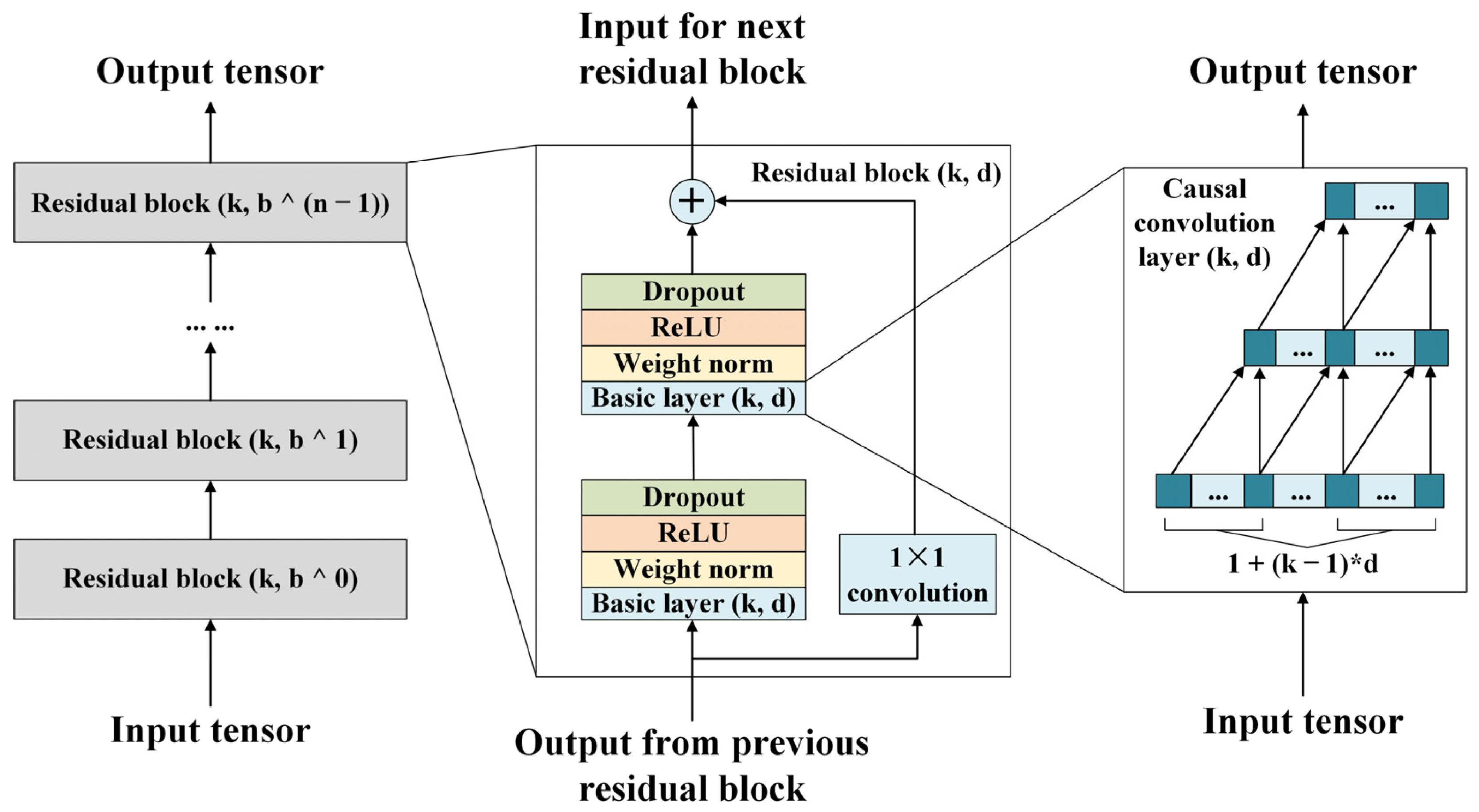
2.3. Temporal Convolutional Network (TCN)

Bai et al. [48] described a family of architectures as a temporal convolutional network (TCN). The TCN has two principles: the length of an input is the same as the output of the network, and future information cannot leak into the past. A generic TCN approach is composed of a 1D fully convolutional network (FCN) and dilated convolutions.

Dilated convolutions enable a receptive field that is exponentially large [49], which is more suitable for longer history sequence tasks. For a 1D sequence input $X\in {\mathbb{R}}^n$ and a filter $f:\{0,\cdots ,k-1\}\to \mathbb{R}$, the dilated convolution operation F is

$$F\left(s\right)=\left(X\ast {}_{d}f\right)\left(s\right)={\displaystyle \sum }_{i=0}^{k-1}f\left(i\right)\cdot X_{s-d\cdot i}$$

(13)

where s is the element of the sequence, d represents the dilation factor, k represents the filter size, and ${}_{s-d\cdot i}$ accounts for the direction of the past.

A residual module (shown in Figure 1) takes the place of a convolution layer in a generic TCN model because layers can learn alterations efficiently to the individuality mapping instead of the whole transformation, especially in very deep networks.

2.4. Prediction Process and Experimental Settings

The mean square error (MSE) was selected as the loss function of the TCN model. Adam [50] was selected as the optimizer in the gradient descent optimization of the stochastic objective function of the TCN model. We set the kernel size as 3, and epochs as 400, respectively.

Landslide cumulative displacement was measured monthly from January 2007 to July 2018 for a total of 144 months. The dataset was separated into three parts: the training, validation, and testing data. The early 96 months from January 2007 to December 2014 made up the training, and the validation data comprised the next 24 months from January 2015 to December 2016. We retained the last 24 months, from January 2017 to December 2018, as the test set.

Firstly, landslide accumulative displacement is decomposed by LMD into two terms: periodic term and trend term. According to Equation (11), the displacement series would be decomposed into PFs and u_k(t). Then, the PFs obtained by LMD are added into a sum sequence, which is considered as the periodic term of the accumulative displacement. The residue u_k(t), which is not oscillating, is considered the trend term. The hyperparameters of displacement predictors should be tuned in the validation set before the test set is used to estimate the performance of the models. The grid search is used to determine the state space of the ETS model and hyperparameters of the TCN model, which are kernel size and dilation. Through the analysis of the monitoring data, the landslide-inducing factors that trigger the periodic displacement are chosen, and the gray relational grade is used to quantitatively determine the correlation between the candidate landslide-inducing factors and periodic displacement.

To predict the displacement of t time in the test set after tuning the hyperparameters, the procedural steps are as follows:

Step 1.

The predicted trend displacement ${\widehat{r}}_t$ is predicted by the ETS model fitting the trend term.

Step 2.

A TCN approach is trained to forecast the landslide-predicted periodic displacement ${\widehat{p}}_t$ based on the periodic term.

Step 3.

The cumulative predicted displacement ${\widehat{s}}_t$ is the sum of the predicted trend displacement ${\widehat{r}}_t$ and the predicted periodic displacement ${\widehat{p}}_t$.

Step 4.

Predict the displacement of t + 1 time by repeating steps 1 to 4.

Figure 2 shows the whole process of landslide displacement prediction.

We contrasted our proposed approach and another existing approach to verify the accuracy of the predicted displacement. According to previous studies [26,51,52], we chose three approaches as benchmarks for comparison: autoregressive integrated moving average (ARIMA), support vector regression (SVR), and long short-term memory neural network (LSTM). The GA was used to tune the hyperparameters of SVR, while grid search was used for ARIMA and LSTM. The details of the parameters are designed in

Table 1. The detailed settings of used models.

Model	Hyperparameter	Explanation
TCN	Kernel size = 3 dilation = 3	Kernel size: The size of every kernel in a convolutional layer. dilation: The base of the exponent determines the dilation on every level.
ARIMA	p = 2 q = 2 d = 0	p: Number of time lags of the autoregressive model (AR). q: The size of the moving average window (MA). d: The order of differentiation.
SVR	C = 518.243 γ = 0.01	C: Regularization parameter. γ: Determine how much influence a single training example has.
LSTM	Hidden layer size = 25	Hidden layer size: Size for each hidden LSTM layer.

. All experimental processes were implemented in Python, and some Python packages were invoked, including Darts [53], scikit-learn [54], and PyTorch [55].

2.5. Metrics

Verifying the models is quite a significant step for prediction accuracy. In this study, mean absolute error (MAE), root mean squared error (RMSE), and coefficient of determination (R²) were used to evaluate the performance of the models [25,26,27,28]. The three metrics above are calculated as presented below.

$$MAE=\frac{1}{n}{\displaystyle \sum }_{i=1}^n\left|{\widehat{y}}_i-y_i\right|$$

(14)

$$RMSE=\sqrt{\frac{1}{n}{\displaystyle \sum }_{i=1}^n{({\widehat{y}}_i-y_i)}^2}$$

(15)

$$R^2=1-\frac{{{\displaystyle \sum }}_{i=1}^n{(y_i-{\widehat{y}}_i)}^2}{{{\displaystyle \sum }}_{i=1}^n{(y_i-\overline{y})}^2}$$

(16)

where y_i and ${\hat{y}}_i$ denote the observed displacement and predicted displacement, respectively, and $\overline{y}$ is the average displacement of n measured displacements. The smaller values of MAE and RMSE show better prediction accuracy and a larger R² represents better prediction accuracy.

3. Case Study

3.1. Topography and Geological Setting

The Baijiabao landslide is sited in Guizhou town, Zigui County, Hubei Province, China, on the west side of the Xiangxi River. The coordinates of latitude and longitude are 30°58′59.9″N, 110°45′33.4″E. The landslide is about 2.5 km upstream of the confluence of the Xiangxi River and the Yangtze River (Figure 3). The primary sliding direction of the Baijiabao landslide is oriented at N 85°E. The shear outlet of the landslide varies in elevation between 125–135 m above sea level, and the toe of the landslide is submerged in the Xiangxi River. The left and right boundaries are identified by bedrock and a gully, respectively. The trailing edge of the landslide is limited by bedrock at an elevation of 265 m. The short tongue-shaped landslide is a width of around 400 m, a length of around 400 m, and an average depth of approximately 45 m, as indicated by boreholes. Hence, the Baijiabao landslide contains 2.2 × 10⁵ m² and has an approximated volume of 9.9 × 10⁶ m³.

This landslide belongs to an anti-dip colluvial landslide (Figure 4) [56]. The landslide mass is composed of loose Quaternary deposits, which are made of greyish-yellow to brownish-yellow gravelly soil, and silty clay with fragmented rubble. The sliding zone is mainly silty clay, which is greyish yellow in the plastic. The lithology of the bedrock is feldspar–quartz sandstone and mudstone, belonging to the Triassic Badong Formation, while Quaternary sediments and soil are noticed under the front of the landslide. The Triassic strata have an approximately 30° dip, and the dip direction is nearly 260°, which is parallel to the landslide surface slope.

3.2. Time Series Monitoring Data and Deformation Analysis

The six global positioning system (GPS) monitoring stations (ZG220, ZG221, ZG323, to ZG326) were installed to monitor the surface displacement in late 2006. The ZG323-ZG326 monitoring stations were established in the middle of the landslide area near the road, whereas ZG220 and ZG221 were established as the datum stations. Hence, monitoring data were obtained from January 2007 to July 2018, as shown in Figure 5. Every time step of the data is one month. The records of four monitoring stations showed step-like characteristics, which meant there was a suddenly increased landslide displacement between April and September (Figure 5).

We chose the Baijiabao landslide as the case study for the following reasons. Firstly, the Baijiabao landslide has been monitored for over ten years, which provided enough time series of high-quality data for training machine-learning models. Four GPS stations in the landslide measured obvious growth of surface displacement, indicating that the landslide is indeed in the stage of deformation. Secondly, the Baijiabao landslide is a typical colluvial landslide in the Three Gorges Reservoir Area. The step-like increase in landslide displacement occurs every summer, which shows the regular distribution. Finally, previous studies [56,57] analyzed the deformation characteristics and triggering factors of the Baijiabao landslide, which provided the basis for our study.

Since the GPS stations were set, the Baijiabao landslide has been continuously deformed. Until December 2018, the maximum displacements recorded by ZG323, ZG324, ZG325, and ZG326 were 1255 mm, 1464 mm, 1362 mm, and 1708 mm, respectively. Except for the largest displacement at the monitoring station, ZG326, located on the right of the Baijiabao landslide, the displacement records of the other three stations were similar, which represented that the Baijiabao landslide deformed synchronously [58].

The increase in landslide displacement shows cyclical regularity. From October to April of the subsequent year, there is a dry season. The displacement increased very slowly in the dry season when the landslide area experienced scarce rainfall, and the reservoir remained at a high level. However, from May to September in the rainy season, when rainfall was rich, the reservoir level was at a low elevation, and the displacement of the landslide increased rapidly, which contributed to over 70% of the yearly displacement to endow the cumulative time–displacement curves with step-like characteristics. For example, the whole-year displacement of ZG324 in 2009 was 199.8 mm, while the monthly displacement of ZG324 between July and August was 97.1 mm and 81.6 mm, which endowed the increase of the annual displacement by 45% and 41%, respectively. The reason is that the increase in precipitation leads to a rise in the underground water level in the landslide body, the decrease in the reservoir water level leads to the water head increasing, and the landslide body produces hydrodynamic pressure directing to the free face and along the path of the landslide, which is detrimental to the landsliding stability. When the reservoir water level is high and the precipitation is low, the hydrodynamic pressure pointing to the slide surface is generated, which makes the landslide stable.

Before the filling of the Three Gorges Reservoir along the Yangtze River, the Baijiaobao landslide had little creep behavior, but obvious deformation behavior was observed after filling [57]. At the head of the landslide, two arcuate tension cracks were observed on the right and left boundaries in June 2007. The right crack was 1–3 cm wide and the left crack was 1–5 cm wide. These cracks were 160 m long and 10 cm deep. Meanwhile, tiny tension cracks were observed near Zi-Xing Road in the middle part of the landslide, which damaged the surface of the road.

In May 2009, heavy rainfall lasting for six days induced many cracks trending N20E to develop along Zi-Xing Road, whose width was approximately 15 cm and depth was approximately 25 cm.

In the head part of the landslide, many large arcuate cracks became interconnected and practically continuous at the landslide boundaries in July 2012. Near the toe of the landslide, the cracks stretched into the reservoir’s hydro-fluctuation belt. In July 2015, new tension cracks, ranging in width from 1 to 5 mm, were discovered at the head of the landslide on the right boundary. There were also a few tension cracks along Zi-Xing Road, particularly where the road crossed the landslide laterally. The cracks ranged in size from 1 to 5 mm in width and 1 to 10 m in length.

We carried out two field surveys in July 2021 and April 2022. In the first field survey, a DJI Matrice 300 RTK Unmanned Aerial Vehicle (UAV) was used to perform 3D modeling of the landslide in Figure 6. The surveys indicated that the landslide currently remained in a relatively stable state. However, with the long-term influence of underground water and reservoir water, especially the sudden increase or decrease in reservoir water, the landslide stability will gradually deteriorate, and it will be unstable at an unknown time point and conditions.

By comparing the deformation characteristics and displacement, we find that the years with obvious cracks are consistent with the years that have large displacement growth (2009, 2012, and 2015). Cracks usually developed on the road in the middle part and near the boundaries of the landslide during the rainy season. The cracks caused the water to easily infiltrate the landslide body, which resulted in a rapid rise in the groundwater level. Therefore, the hydrodynamic pressure was increased, reducing the effective stress on the landsliding mass movement. In addition, long-term saturation would reduce the mechanical strength of the soil. These reasons explain why developed cracks cause landslide displacement to increase.

4. Results

4.1. Cumulative Displacement Decomposition

We decomposed four GPS monitoring stations of the Baijiabao landslide cumulative displacement by LMD. The PFs of each station’s cumulative displacement were regarded as the periodic displacement, and the residue of each station was considered as trend displacement (Figure 7). The trend displacement showed the increased tendency of the developing displacement without the step-like characteristic, and the periodic displacement changed over time as a time series.

4.2. Trend Displacement Prediction

First, the grid search was used to determine the state space of the ETS model before predicting trend displacement. Then, we trained each kind of ETS model in the training set, and the AIC corrected for small sample bias (AIC_C) was used here to decide which of the ETS models was most suitable (shown in

Table 2. The AIC_C results of the trend displacement in four GPS stations.

	ZG323	ZG324	ZG325	ZG326
ETS (A, A, N)	398.164	388.168	371.580	353.010
ETS (A, Ad, N)	399.886	391.479	373.780	358.070
ETS (A, A, M)	401.779	419.033	653.940	390.110
ETS (A, Ad, M)	405.402	443.103	407.100	395.750
ETS (M, A, N)	407.325	957.639	500.880	470.510
ETS (A, A, A)	408.013	417.567	653.730	386.480
ETS (M, Ad, N)	408.481	1033.737	512.030	479.280
ETS (A, Ad, A)	410.877	421.896	406.080	392.370
ETS (M, A, A)	418.297	946.128	515.820	480.750
ETS (M, A, M)	429.235	776.559	532.780	500.510
ETS (M, Ad, A)	431.305	523.652	528.800	491.650
ETS (M, Ad, M)	441.487	783.988	544.840	510.350
ETS (A, N, N)	714.137	740.008	728.970	765.490
ETS (A, N, M)	742.629	775.787	761.540	797.760
ETS (A, N, A)	744.536	771.705	761.480	798.000
ETS (M, N, N)	746.094	1024.060	819.330	798.650
ETS (M, N, A)	777.466	876.940	848.900	827.650
ETS (M, N, M)	778.535	985.622	851.510	830.750

).

The results show that the ETS (A, A, N) was most appropriate for trend displacement. The curves of the predicted trend displacement are exhibited in Figure 8, and the performance of the results are demonstrated in

Table 3. The predicted accuracy for the training models.

	MAE	RMSE	R2
ZG323	0.645	0.831	0.999
ZG324	2.071	2.425	0.998
ZG325	1.072	1.448	0.999
ZG326	2.323	2.961	0.999

by ETS (A, A, N). ETS (A, A, N) showed the best performance in ZG323, and the MAE, RMSE, and R² of the ZG323 trend displacement were 0.646, 0.831, and 0.999, respectively.

4.3. Periodic Displacement Prediction

4.3.1. Selection of Inducing Factors

Precipitation is one of the major inducing factors triggering landslides in the TGRA [59,60]. On one hand, rainfall seeps into rock fractures and soil porosity to cause the underground water level to rise in the landslide body, which softens the rock and soil and decreases the shear strength on the surface of the rupture. Therefore, the resisting forces are reduced. On the other hand, seeped water increases the weight of the landslide body, which leads to enhancing the driving forces. Thus, the landslide becomes unstable, increasing the landslide displacement [61]. The periodic displacement of the Baijiabao landslide fluctuated with the variation in numerous external inducing factors. Figure 9 shows that the monthly precipitation had a positive correlation with the periodic displacement rate, while the cyclicity of displacement exhibited a slight lag hysteresis compared to the cyclicity of monthly precipitation. A possible explanation for this might be that the landslide maintained a stable state when rainfall did not exceed a threshold [62]. The fluctuation in reservoir level also had an important effect on the deformation of landslides [26]. As illustrated in Figure 9, as the reservoir water level rose, the periodic displacement decreased. When the reservoir water level remained stable, the periodic displacement tended to be steady. In general, cyclical fluctuations in the reservoir water level should lead to fluctuations in periodic displacement. Reservoir level fluctuation and rainfall are typically the major landslide-inducing factors that influence the displacement of the step-like reservoir bank landslide. Consequently, the key to accurate periodic displacement prediction is the selection of influencing factors [63]. Precipitation and reservoir water level have a lag effect on the landslide periodic displacement, and the landslide periodic displacement also has autocorrelation. Referring to other research [27,64], we selected the periodic displacement, precipitation, and reservoir water level over the past three months as landslide-inducing factors. The gray relational grade (GRG) was used to assess the relationship between landslide-inducing factors and periodic displacement as shown in

Table 4. Input data for the approaching of the periodic displacement and the GRA between inducing factors and periodic displacement.

	ZG323	ZG324	ZG325	ZG326
Periodic displacement over one month	0.863	0.906	0.877	0.891
Periodic displacement over two months	0.778	0.845	0.795	0.820
Periodic displacement over three months	0.715	0.794	0.733	0.766
Precipitation in the current month	0.687	0.731	0.774	0.897
Precipitation in the previous month	0.706	0.746	0.751	0.844
Precipitation in the two months before	0.729	0.761	0.788	0.915
Reservoir level in the current month	0.725	0.749	0.760	0.734
Reservoir level in the previous month	0.671	0.716	0.717	0.695
Reservoir level in the two months before	0.614	0.679	0.675	0.658

.

4.3.2. The TCN Prediction of Periodic Displacement

Table 5. Prediction accuracy of periodic displacement in ZG323 to ZG326.

	MAE	RMSE	R2
ZG323	10.423	13.061	0.602
ZG324	13.133	16.938	0.650
ZG325	9.795	14.663	0.694
ZG326	17.371	21.005	0.850

demonstrates the accuracy of the predicted results of the TCN model at four GPS stations. Figure 10 shows that the predicted values were close to the measured displacement of the periodic term. However, at the maximum and minimum points of the periodic displacement, the predicted accuracy shows obvious errors. For example, in ZG323 from July 2017 to August 2017, the displacement of the periodic term increased from −28.6 mm to 28.7 mm. Such a sudden shift reduced the prediction accuracy of the TCN and caused the model to overestimate the periodic displacement of the following month (September 2017). Similarly, in ZG324 from July 2017 to August 2017 and from July 2018 to August 2018, the periodic displacement increased suddenly, resulting in poor accuracy of the periodic displacement in these periods and one month later. In the summers of 2017 and 2018, the periodic displacement increased suddenly and rapidly from the bottom to the head. Due to the large displacement changes, the displacement prediction in this period had a large error and showed a lag effect.

4.4. Cumulative Displacement Prediction

We used SVR, ARIMA, and LSTM to predict periodic landslide displacement from ZG323 to ZG326 GPS monitoring stations as compared to models. Adding the trend displacement to the periodic displacement, the predicted values of cumulative displacement were obtained. Figure 11 presents the predicted cumulative displacement of ZG323 to ZG326 Baijiabao GPS stations in the test set from January 2017 to December 2018. In

Table 6. Prediction accuracy of cumulative displacement in ZG323 to ZG326.

	MAE	RMSE	R2
ZG323	10.340	12.821	0.927
ZG324	13.615	17.545	0.907
ZG325	9.720	14.854	0.915
ZG326	17.314	21.380	0.896

, we can see the evaluation index of each station.

5. Discussion

Analyzing the error of the results assists us to find the regularities of prediction accuracy. According to Figure 11 and

Table 7. Cumulative displacement of accuracy assessment with different predicted models in ZG323 to ZG326.

		MAE	RMSE	R2
ZG323	ARIMA	11.732	15.224	0.897
	SVR	15.348	17.637	0.862
	LSTM	11.584	14.836	0.902
	TCN	10.340	12.821	0.927
ZG324	ARIMA	16.371	20.225	0.876
	SVR	14.393	18.993	0.891
	LSTM	13.615	17.545	0.907
	TCN	9.140	13.800	0.942
ZG325	ARIMA	13.106	17.410	0.883
	SVR	15.183	21.029	0.829
	LSTM	12.759	19.825	0.848
	TCN	9.720	14.854	0.915
ZG326	ARIMA	24.300	30.726	0.785
	SVR	23.056	26.120	0.845
	LSTM	18.797	24.616	0.862
	TCN	17.314	21.381	0.896

, TCN was the best-performing model, the secondary performance model was LSTM, and ARIMA performed better than SVR in ZG323 and ZG325 but worse in ZG324 and ZG326. Compared with ARIMA, SVR, and LSTM, the accuracy of TCN was improved by an average of 40.9%, 46.2%, and 22.1%, respectively. This indicates that the robustness of the TCN approach has the best performance.

The MAE, RMSE, and R² represent the metrics for evaluating the mean error of the total predicted displacement values, but the bias of the predicted values should also be considered. Boxplots of absolute errors in Figure 12 show the discrete distribution and skewness in ZG323 to ZG326. Although the extreme value of the error is not always the smallest, the interquartile range (IQR) of the TCN is always the smallest among the four GPS stations.

ARIMA is a classical time series forecasting model; however, by comparing the prediction accuracy of four GPS monitoring stations, it is found that their performance is not stable enough. In ZG323, the ARIMA-predicted accuracy is higher than that of the SVR model and close to that of the LSTM model. However, ARIMA is the worst-performing model in ZG324 and ZG326. The reason may be that ARIMA is a univariate prediction model and cannot input multiple influencing factors. ZG324 and ZG326 are two GPS stations with larger displacement increases. Therefore, larger displacement increases are more likely to lead to the lower predicted accuracy of the univariate model. The prediction curve of SVR was linear and did not show the characteristics of sharply increasing step-like displacement. This may be due to several reasons: although the optimization algorithms were used, it was difficult to acquire ideal values for SVR’s hyperparameters because of the lack of prior knowledge. SVR relies on a split of the training data because the training data within the loss function are disregarded. The local predicted accuracy of SVR in the neighborhood of the training points has a limitation on account of noticeable deviations between actual responses and estimated responses at the training points [65].

In addition, as shown in Table 7 and Figure 12, the predicted accuracy of LSTM is only worse than that of TCN, but the bias of predicted displacement values is higher than that of TCN. Its interquartile range is wider than that of the TCN. Overall, the prediction accuracy of LSTM is the second highest after TCN. Both LSTM and TCN are deep-learning models, and their prediction accuracy is higher than that of the classical statistical model ARIMA and the classical machine-learning model SVR. Moreover, it is shown that deep-learning models designed for sequential data could outperform traditional statistical models and machine learning on small samples.

As seen in Figure 11, sharply step-like increased landslide displacement of four GPS stations occurred in July 2017 and in July 2018, which were in the latter half of the year. The predicted landslide displacement values became inaccurate after sharp increases in landslide displacement occurred. Therefore, we split the predicted values by every half of the year and then compared the metrics of the first half of the year and the latter half of the year. The results shown in

Table 8. Comparison of accuracy between the first half and latter half of the years.

		MAE		RMSE		R2
		First Half of Years	Latter Half of Years	First Half of Years	Latter Half of Years	First Half of Years	Latter Half of Years
ZG323	ARIMA	9.731	13.734	10.889	18.574	0.896	0.786
	SVR	14.161	16.535	16.395	18.796	0.763	0.781
	LSTM	8.179	14.989	9.731	18.589	0.917	0.785
	TCN	8.014	12.667	9.683	15.329	0.917	0.854
ZG324	ARIMA	13.375	19.366	17.030	22.981	0.826	0.790
	SVR	9.768	19.017	11.947	24.057	0.915	0.770
	LSTM	11.344	15.886	13.374	20.899	0.893	0.826
	TCN	5.870	12.410	7.549	17.992	0.966	0.871
ZG325	ARIMA	8.528	17.683	9.788	22.593	0.930	0.748
	SVR	8.899	21.467	11.134	27.576	0.910	0.624
	LSTM	8.599	16.920	10.254	26.095	0.924	0.664
	TCN	4.455	14.985	5.672	20.227	0.977	0.798
ZG326	ARIMA	12.523	36.077	14.776	40.864	0.909	0.526
	SVR	20.493	25.619	23.386	28.594	0.771	0.768
	LSTM	12.074	25.520	13.803	31.959	0.920	0.710
	TCN	8.963	25.664	10.091	28.503	0.957	0.769

represent that the metrics in the latter half of the year are less than half of those in the first half of the year. The increase in displacement from July to September contributed to over 90% of the yearly displacement to endow the cumulative time–displacement curves with step-like characteristics. The RMSE of ARIMA, SVR, LSTM, and TCN from July to September were 32.027, 25.408, 31.537, and 24.342, respectively, which were bigger than RMSE in the test set. It confirmed that the step-like period of the landslide conducted large, predicted errors. Consequently, the performance of landslide displacement does not only rely on the beginning and the end of sharply increased landslide displacement.

We used the LMD–ETS–TCN model in four Baijiabao landslide stations from ZG323 to ZG326. The predicted performance is ZG323>ZG325>ZG324>ZG326, which is the same in cumulative, trend, and periodic displacement. The step-like increased displacement in the rainy season contributed over 70% of the annual displacement in Figure 5. Therefore, it may be that the model performs worse in the unstable part of the landslide. Compared with the metrics of trend displacement (Table 3), periodic displacement (Table 5), and cumulative displacement (Table 6), the predicted errors were mainly from periodic displacement.

As mentioned above, the main predicted errors resulted from periodic displacement and occurred in sharp displacement in the latter half of the years. Moreover, the predicted displacement had a lag period that delayed the measured displacement. Some previous studies have tried to improve the accuracy of sharply increased displacement by using ensemble learning and feature engineering [61,64], which could provide some inspiration.

In recent research, models updating constantly can only ensure prediction of the future landslide displacement in a finite period. Reservoir level and rainfall mainly affect landslide displacement through groundwater, which is an indirect process. Therefore, rainfall and reservoir level may not be very relevant to landslide displacement. The monitoring of landslide displacement widely uses the global positioning system (GPS) in a landslide early warning and long-term monitoring systems [66]. However, only surface displacements can be obtained using GPS, and environmental variation has a significant impact on measuring accuracy [67,68,69]. With development, the monitoring system should record more correlative landslide-inducing factors, such as underground water and deep displacement, the monitoring frequency should be shortened to days and hours, and feature engineering should be carried out through big data analysis to select and analyze the factors that are more relevant to the impact of landslide displacement, geology, and the mechanical mechanism of displacement.

6. Conclusions

To sustain landslide early warning, this paper proposed a hybrid model named LMD–ETS–TCN to predict landslide cumulative displacement. Compared with other approaches, including ARIMA, SVR, and LSTM, the TCN model has the best performance, not only in prediction accuracy but also in prediction bias, at four time-series GPS monitoring stations of the Baijiabao landslide in the TGRA region. Meanwhile, we found that the deep-learning models were better than the traditional models. Considering that the total sample size was only 144, this result showed that deep-learning models designed for sequential data could outperform traditional machine learning even on small samples. By comparison, it was found that the errors were mainly obtained from periodic displacement prediction. Furthermore, it was also found that the more unstable part of the landslide may lead to worse prediction accuracy. During the step-like period of the landslide, the displacement sequence increased rapidly from minimum to maximum, resulting in a large predicted error. Hence, future research into landslide displacement prediction should focus on the step-like period. In the step-like period, studies are required to gain more time series monitoring data, which are more correlative landslide-inducing factors, such as underground water and deep displacement, to explore the law of landslide evolution.

References

1. Dou, J.; Yunus, A.P.; Merghadi, A.; Shirzadi, A.; Nguyen, H.; Hussain, Y.; Avtar, R.; Chen, Y.; Pham, B.T.; Yamagishi, H. Different Sampling Strategies for Predicting Landslide Susceptibilities Are Deemed Less Consequential with Deep Learning. Sci. Total Environ. 2020, 720, 137320. [Google Scholar] [CrossRef] [PubMed]
2. Li, H.; Xu, Y.; Zhou, J.; Wang, X.; Yamagishi, H.; Dou, J. Preliminary Analyses of a Catastrophic Landslide Occurred on 23 July 2019, in Guizhou Province, China. Landslides 2020, 17, 719–724. [Google Scholar] [CrossRef]
3. Dou, J.; Yunus, A.P.; Tien Bui, D.; Merghadi, A.; Sahana, M.; Zhu, Z.; Chen, C.W.; Khosravi, K.; Yang, Y.; Pham, B.T. Assessment of Advanced Random Forest and Decision Tree Algorithms for Modeling Rainfall-Induced Landslide Susceptibility in the Izu-Oshima Volcanic Island, Japan. Sci. Total Environ. 2019, 662, 332–346. [Google Scholar] [CrossRef] [PubMed]
4. Merghadi, A.; Yunus, A.P.; Dou, J.; Whiteley, J.; ThaiPham, B.; Bui, D.T.; Avtar, R.; Abderrahmane, B. Machine Learning Methods for Landslide Susceptibility Studies: A Comparative Overview of Algorithm Performance. Earth-Science Rev. 2020, 207, 103225. [Google Scholar] [CrossRef]
5. Wang, W.; He, Z.; Han, Z.; Li, Y.; Dou, J.; Huang, J. Mapping the Susceptibility to Landslides Based on the Deep Belief Network: A Case Study in Sichuan Province, China. Nat. Hazards 2020, 103, 3239–3261. [Google Scholar] [CrossRef]
6. Wang, F.; Li, T. Landslide Disaster Mitigation in Three Gorges Reservoir, China; Springer: Berlin/Heidelberg, Germany, 2009. [Google Scholar]
7. Wang, F.-W.; Zhang, Y.-M.; Huo, Z.-T.; Matsumoto, T.; Huang, B.-L. The 14 July 2003 Qianjiangping Landslide, Three Gorges Reservoir, China. Landslides 2004, 1, 157–162. [Google Scholar] [CrossRef]
8. Tang, H.; Wasowski, J.; Juang, C.H. Geohazards in the Three Gorges Reservoir Area, China—Lessons Learned from Decades of Research. Eng. Geol. 2019, 261, 105267. [Google Scholar] [CrossRef]
9. Cojean, R.; Caï, Y.J. Analysis and Modeling of Slope Stability in the Three-Gorges Dam Reservoir (China)—The Case of Huangtupo Landslide. J. Mt. Sci. 2011, 8, 166–175. [Google Scholar] [CrossRef]
10. Yin, Y.; Wang, H.; Gao, Y.; Li, X. Real-Time Monitoring and Early Warning of Landslides at Relocated Wushan Town, the Three Gorges Reservoir, China. Landslides 2010, 7, 339–349. [Google Scholar] [CrossRef]
11. Petley, D.N.; Mantovani, F.; Bulmer, M.H.; Zannoni, A. The Use of Surface Monitoring Data for the Interpretation of Landslide Movement Patterns. Geomorphology 2005, 66, 133–147. [Google Scholar] [CrossRef]
12. Guzzetti, F.; Gariano, S.L.; Peruccacci, S.; Brunetti, M.T.; Marchesini, I.; Rossi, M.; Melillo, M. Geographical Landslide Early Warning Systems. Earth-Science Rev. 2020, 200, 102973. [Google Scholar] [CrossRef]
13. Liu, L.-L.; Zhang, J.; Li, J.-Z.; Huang, F.; Wang, L.-C. A Bibliometric Analysis of the Landslide Susceptibility Research (1999–2021). Geocarto Int. 2022, 1–26. [Google Scholar] [CrossRef]
14. Huang, S.-Y.; Zhang, S.-H.; Liu, L.-L. A New Active Learning Kriging Metamodel for Structural System Reliability Analysis with Multiple Failure Modes. Reliab. Eng. Syst. Saf. 2022, 228, 108761. [Google Scholar] [CrossRef]
15. Saito, M. Forecasting the Time of Occurrence of a Slope Failure. In Proceedings of the 6th International Conference on Soil Mechanics and Foundation Engineering, Montreal, QC, USA, 8–15 September 1965; pp. 537–541. [Google Scholar]
16. Li, X.; Kong, J.; Wang, Z. Landslide Displacement Prediction Based on Combining Method with Optimal Weight. Nat. Hazards 2012, 61, 635–646. [Google Scholar] [CrossRef]
17. Saito, M. Forecasting Time of Slope Failure by Tertiary Creep. In Proceedings of the 7th International Conference on Soil Mechanics and Foundation Engineering, Mexico City, Mexico, 29 August 1969; Volume 2, pp. 677–683. [Google Scholar]
18. Voight, B. A Relation to Describe Rate-Dependent Material Failure. Science 1989, 243, 200–203. [Google Scholar] [CrossRef] [PubMed] [Green Version]
19. Li, T.B.; Chen, M.D.; Wang, L.S. Landslide Real-Time Tracking Prediction; Chengdu University of Science and Technology Press: Chengdu, China, 1999; pp. 27–31. [Google Scholar]
20. Lu, P.; Rosenbaum, M.S. Artificial Neural Networks and Grey Systems for the Prediction of Slope Stability. Nat. Hazards 2003, 30, 383–398. [Google Scholar] [CrossRef]
21. Du, J.; Yin, K.; Lacasse, S. Displacement Prediction in Colluvial Landslides, Three Gorges Reservoir, China. Landslides 2013, 10, 203–218. [Google Scholar] [CrossRef]
22. Huang, F.; Yin, K.; Zhang, G.; Gui, L.; Yang, B.; Liu, L. Landslide Displacement Prediction Using Discrete Wavelet Transform and Extreme Learning Machine Based on Chaos Theory. Environ. Earth Sci. 2016, 75, 1376. [Google Scholar] [CrossRef]
23. Cai, Z.; Xu, W.; Meng, Y.; Shi, C.; Wang, R. Prediction of Landslide Displacement Based on GA-LSSVM with Multiple Factors. Bull. Eng. Geol. Environ. 2016, 75, 637–646. [Google Scholar] [CrossRef]
24. Chen, H.; Zeng, Z.; Tang, H. Landslide Deformation Prediction Based on Recurrent Neural Network. Neural Process. Lett. 2015, 41, 169–178. [Google Scholar] [CrossRef]
25. Zhang, K.; Zhang, K.; Cai, C.; Liu, W.; Xie, J. Displacement Prediction of Step-like Landslides Based on Feature Optimization and VMD-Bi-LSTM: A Case Study of the Bazimen and Baishuihe Landslides in the Three Gorges, China. Bull. Eng. Geol. Environ. 2021, 80, 8481–8502. [Google Scholar] [CrossRef]
26. Yang, B.; Yin, K.; Lacasse, S.; Liu, Z. Time Series Analysis and Long Short-Term Memory Neural Network to Predict Landslide Displacement. Landslides 2019, 16, 677–694. [Google Scholar] [CrossRef]
27. Xu, S.; Niu, R. Displacement Prediction of Baijiabao Landslide Based on Empirical Mode Decomposition and Long Short-Term Memory Neural Network in Three Gorges Area, China. Comput. Geosci. 2018, 111, 87–96. [Google Scholar] [CrossRef]
28. Long, J.; Li, C.; Liu, Y.; Feng, P.; Zuo, Q. A Multi-Feature Fusion Transfer Learning Method for Displacement Prediction of Rainfall Reservoir-Induced Landslide with Step-like Deformation Characteristics. Eng. Geol. 2022, 297, 106494. [Google Scholar] [CrossRef]
29. Dou, J.; Xiang, Z.; Qiang, X.; Zheng, P.; Wang, X.; Su, A.; Liu, J.; Luo, W. Application and Development Trend of Machine Learning in Landslide Intelligent Disaster Prevention and Mitigation. Earth Sci. 2022. [Google Scholar] [CrossRef]
30. Pham, B.T.; Nguyen-Thoi, T.; Qi, C.; Van Phong, T.; Dou, J.; Ho, L.S.; Van Le, H.; Prakash, I. Coupling RBF Neural Network with Ensemble Learning Techniques for Landslide Susceptibility Mapping. Catena 2020, 195, 104805. [Google Scholar] [CrossRef]
31. Jiang, Y.; Luo, H.; Xu, Q.; Lu, Z.; Liao, L.; Li, H.; Hao, L. A Graph Convolutional Incorporating GRU Network for Landslide Displacement Forecasting Based on Spatiotemporal Analysis of GNSS Observations. Remote Sens. 2022, 14, 1016. [Google Scholar] [CrossRef]
32. Xu, Q.; Tang, M.G.; Xu, K.X.; Huang, X. Research on Space-Time Evolution Laws and Early Warning-Prediction of Landslides. Chin. J. Rock Mech. Eng. 2008, 27, 1104–1112. [Google Scholar]
33. Wang, J.F. Quantitative Prediction of Landslide Using S-Curve. Chin. J. Geol. Hazard Control 2003, 14, 1–8. [Google Scholar]
34. Du, H.; Song, D.Q.; Chen, Z.; Shu, H.P.; Guo, Z.Z. Prediction Model Oriented for Landslide Displacement with Step-like Curve by Applying Ensemble Empirical Mode Decomposition and the PSO-ELM Method. J. Clean. Prod. 2020, 270, 122248. [Google Scholar] [CrossRef]
35. Li, C.; Criss, R.E.; Fu, Z.; Long, J.; Tan, Q. Evolution Characteristics and Displacement Forecasting Model of Landslides with Stair-Step Sliding Surface along the Xiangxi River, Three Gorges Reservoir Region, China. Eng. Geol. 2021, 283, 105961. [Google Scholar] [CrossRef]
36. Zhang, Y.; Tang, J.; He, Z.; Tan, J.; Li, C. A Novel Displacement Prediction Method Using Gated Recurrent Unit Model with Time Series Analysis in the Erdaohe Landslide. Nat. Hazards 2021, 105, 783–813. [Google Scholar] [CrossRef]
37. Zhang, L.G.; Chen, X.Q.; Zhang, Y.G.; Wu, F.W.; Chen, F.; Wang, W.T.; Guo, F. Application of GWO-ELM Model to Prediction of Caojiatuo Landslide Displacement in the Three Gorge Reservoir Area. Water 2020, 12, 1860. [Google Scholar] [CrossRef]
38. Chou, Y. Statistical Analysis: With Business and Economic Applications; Holt, Rinehart and Winston: New York, NY, USA, 1975; ISBN 9780030854040. [Google Scholar]
39. Zhou, C.; Yin, K.; Cao, Y.; Ahmed, B. Application of Time Series Analysis and PSO–SVM Model in Predicting the Bazimen Landslide in the Three Gorges Reservoir, China. Eng. Geol. 2016, 204, 108–120. [Google Scholar] [CrossRef]
40. Guo, Z.; Chen, L.; Gui, L.; Du, J.; Yin, K.; Do, H.M. Landslide Displacement Prediction Based on Variational Mode Decomposition and WA-GWO-BP Model. Landslides 2020, 17, 567–583. [Google Scholar] [CrossRef]
41. Lin, Z.; Ji, Y.; Liang, W.; Sun, X. Landslide Displacement Prediction Based on Time-Frequency Analysis and LMD-BiLSTM Model. Mathematics 2022, 10, 2203. [Google Scholar] [CrossRef]
42. Zhu, X.; Zhang, F.; Deng, M.; Liu, J.; He, Z.; Zhang, W.; Gu, X. A Hybrid Machine Learning Model Coupling Double Exponential Smoothing and ELM to Predict Multi-Factor Landslide Displacement. Remote Sens. 2022, 14, 3384. [Google Scholar] [CrossRef]
43. Zhu, X.; Xu, Q.; Tang, M.G.; Nie, W.; Ma, S.Q.; Xu, Z.P. Comparison of Two Optimized Machine Learning Models for Predicting Displacement of Rainfall-Induced Landslide: A Case Study in Sichuan Province, China. Eng. Geol. 2017, 218, 213–222. [Google Scholar] [CrossRef]
44. Huang, D.; He, J.; Song, Y.; Guo, Z.; Huang, X.; Guo, Y. Displacement Prediction of the Muyubao Landslide Based on a GPS Time-Series Analysis and Temporal Convolutional Network Model. Remote Sens. 2022, 14, 2656. [Google Scholar] [CrossRef]
45. Zhang, D.; Yang, J.; Li, F.; Han, S.; Qin, L.; Li, Q. Landslide Risk Prediction Model Using an Attention-Based Temporal Convolutional Network Connected to a Recurrent Neural Network. IEEE Access 2022, 10, 37635–37645. [Google Scholar] [CrossRef]
46. Smith, J.S. The Local Mean Decomposition and Its Application to EEG Perception Data. J. R. Soc. Interface 2005, 2, 443–454. [Google Scholar] [CrossRef] [PubMed]
47. Hyndman, R.J.; Athanasopoulos, G. Forecasting: Principles and Practice; OTexts: Melbourne, VIC, Australia, 2018. [Google Scholar]
48. Bai, S.; Kolter, J.Z.; Koltun, V. An Empirical Evaluation of Generic Convolutional and Recurrent Networks for Sequence Modeling. arXiv 2018, arXiv:1803.01271. [Google Scholar]
49. Yu, F.; Koltun, V. Multi-Scale Context Aggregation by Dilated Convolutions. arXiv 2015, arXiv:1511.07122. [Google Scholar]
50. Kingma, D.P.; Ba, J. Adam: A Method for Stochastic Optimization. arXiv 2014, arXiv:1412.6980. [Google Scholar]
51. Li, X.Z.; Kong, J.M. Application of GA–SVM Method with Parameter Optimization for Landslide Development Prediction. Nat. Hazards Earth Syst. Sci. 2014, 14, 525–533. [Google Scholar] [CrossRef]
52. Miao, F.; Wu, Y.; Xie, Y.; Li, Y.; Fan, B.; Zhang, J. Displacement Prediction of Baishuihe Landslide Based on Multi Algorithm Optimization and SVR Model. J. Eng. Geol. 2016, 24, 1136–1144. [Google Scholar]
53. Herzen, J.; Lässig, F.; Piazzetta, S.G.; Neuer, T.; Tafti, L.; Raille, G.; Van Pottelbergh, T.; Pasieka, M.; Skrodzki, A.; Huguenin, N.; et al. Darts: User-Friendly Modern Machine Learning for Time Series. 2021. [Google Scholar]
54. Pedregosa, F.; Varoquaux, G.; Gramfort, A.; Michel, V.; Thirion, B.; Grisel, O.; Blondel, M.; Prettenhofer, P.; Weiss, R.; Dubourg, V.; et al. Scikit-Learn: Machine Learning in Python. J. Mach. Learn. Res. 2011, 12, 2825–2830. [Google Scholar]
55. Paszke, A.; Gross, S.; Massa, F.; Lerer, A.; Bradbury, J.; Chanan, G.; Killeen, T.; Lin, Z.; Gimelshein, N.; Antiga, L.; et al. Pytorch: An Imperative Style, High-Performance Deep Learning Library. Adv. Neural Inf. Process. Syst. 2019, 32. [Google Scholar]
56. Yao, W.; Li, C.; Zuo, Q.; Zhan, H.; Criss, R.E. Spatiotemporal Deformation Characteristics and Triggering Factors of Baijiabao Landslide in Three Gorges Reservoir Region, China. Geomorphology 2019, 343, 34–47. [Google Scholar] [CrossRef]
57. Wu, X.; Benjamin Zhan, F.; Zhang, K.; Deng, Q. Application of a Two-Step Cluster Analysis and the Apriori Algorithm to Classify the Deformation States of Two Typical Colluvial Landslides in the Three Gorges, China. Environ. Earth Sci. 2016, 75, 146. [Google Scholar] [CrossRef]
58. Cao, Y.; Yin, K.; Alexander, D.E.; Zhou, C. Using an Extreme Learning Machine to Predict the Displacement of Step-like Landslides in Relation to Controlling Factors. Landslides 2016, 13, 725–736. [Google Scholar] [CrossRef]
59. Tomás, R.; Li, Z.; Liu, P.; Singleton, A.; Hoey, T.; Cheng, X. Spatiotemporal Characteristics of the Huangtupo Landslide in the Three Gorges Region (China) Constrained by Radar Interferometry. Geophys. J. Int. 2014, 197, 213–232. [Google Scholar] [CrossRef] [Green Version]
60. Yang, B.; Yin, K.; Xiao, T.; Chen, L.; Du, J. Annual Variation of Landslide Stability under the Effect of Water Level Fluctuation and Rainfall in the Three Gorges Reservoir, China. Environ. Earth Sci. 2017, 76, 564. [Google Scholar] [CrossRef]
61. Zhang, J.; Tang, H.; Wen, T.; Ma, J.; Tan, Q.; Xia, D.; Liu, X.; Zhang, Y. A Hybrid Landslide Displacement Prediction Method Based on CEEMD and DTW-ACO-SVR—Cases Studied in the Three Gorges Reservoir Area. Sensors 2020, 20, 4287. [Google Scholar] [CrossRef] [PubMed]
62. Segoni, S.; Piciullo, L.; Gariano, S.L. A Review of the Recent Literature on Rainfall Thresholds for Landslide Occurrence. Landslides 2018, 15, 1483–1501. [Google Scholar] [CrossRef]
63. Zhang, L.; Shi, B.; Zhu, H.; Yu, X.B.; Han, H.; Fan, X. PSO-SVM-Based Deep Displacement Prediction of Majiagou Landslide Considering the Deformation Hysteresis Effect. Landslides 2021, 18, 179–193. [Google Scholar] [CrossRef]
64. Han, H.; Shi, B.; Zhang, L. Prediction of Landslide Sharp Increase Displacement by SVM with Considering Hysteresis of Groundwater Change. Eng. Geol. 2021, 280, 105876. [Google Scholar] [CrossRef]
65. Yan, C.; Shen, X.; Guo, F.; Zhao, S.; Zhang, L. A Novel Model Modification Method for Support Vector Regression Based on Radial Basis Functions. Struct. Multidiscip. Optim. 2019, 60, 983–997. [Google Scholar] [CrossRef]
66. Akbarimehr, M.; Motagh, M.; Haghshenas-Haghighi, M. Slope Stability Assessment of the Sarcheshmeh Landslide, Northeast Iran, Investigated Using InSAR and GPS Observations. Remote Sens. 2013, 5, 3681–3700. [Google Scholar] [CrossRef] [Green Version]
67. Zou, Z.; Yan, J.; Tang, H.; Wang, S.; Xiong, C.; Hu, X. A Shear Constitutive Model for Describing the Full Process of the Deformation and Failure of Slip Zone Soil. Eng. Geol. 2020, 276, 105766. [Google Scholar] [CrossRef]
68. Wang, J.; Schweizer, D.; Liu, Q.; Su, A.; Hu, X.; Blum, P. Three-Dimensional Landslide Evolution Model at the Yangtze River. Eng. Geol. 2021, 292, 106275. [Google Scholar] [CrossRef]
69. Tang, H.; Li, C.; Hu, X.; Su, A.; Wang, L.; Wu, Y.; Criss, R.; Xiong, C.; Li, Y. Evolution Characteristics of the Huangtupo Landslide Based on in Situ Tunneling and Monitoring. Landslides 2015, 12, 511–521. [Google Scholar] [CrossRef]
Figure 1. The structural design of the TCN.
Remotesensing 15 00229 g001
Figure 2. Flowchart of the proposed approach for landslide displacement prediction.
Remotesensing 15 00229 g002
Figure 3. Location and GPS monitoring stations of the case study.
Remotesensing 15 00229 g003
Figure 4. Geological profile of the case study.
Remotesensing 15 00229 g004
Figure 5. Precipitation, reservoir level, and measured cumulative displacement in the Baijiabao landslide: white fill—dry season; gray fill—rainy season.
Remotesensing 15 00229 g005
Figure 6. UAV field survey: (a) UAV 3D modeling of the landslide in July 2021; (b) a crack in the landslide; (c) a gully in the landslide.
Remotesensing 15 00229 g006
Figure 7. (a) Cumulative displacement of four GPS stations; (b) trend displacement of four GPS stations by LMD; (c) periodic displacement of four GPS stations by LMD.
Remotesensing 15 00229 g007
Figure 8. (a) Predicted and observed trend displacement in the test set of ZG323; (b) predicted and measured trend displacement of ZG324; (c) predicted and measured trend displacement of ZG325; (d) predicted and measured trend displacement of ZG326.
Remotesensing 15 00229 g008
Figure 9. Precipitation, reservoir level, and periodic displacement rate in ZG323 to ZG326. White fill—dry season; gray fill—rainy season.
Remotesensing 15 00229 g009
Figure 10. (a) The TCN prediction of periodic displacement in ZG323; (b) the TCN prediction of periodic displacement in ZG324; (c) the TCN prediction of periodic displacement in ZG325; (d) the TCN prediction of periodic displacement in ZG326.
Remotesensing 15 00229 g010
Figure 11. (a) Comparison of different models for cumulative displacement in ZG323; (b) comparison of different models for cumulative displacement in ZG324; (c) comparison of different models for cumulative displacement in ZG325; (d) comparison of different models for cumulative displacement in ZG326.
Remotesensing 15 00229 g011
Figure 12. (a) Boxplots of absolute predicted errors for each model in ZG323; (b) boxplots of absolute predicted errors for each model in ZG324; (c) boxplots of absolute predicted errors for each model in ZG325; (d) boxplots of absolute predicted errors for each model in ZG326, the points represent the outliers.
Remotesensing 15 00229 g012