Modeling and Forecasting Ionospheric foF2 Variation in the Low Latitude Region during Low and High Solar Activity Years

Abstract

Prediction of ionospheric parameters, such as ionospheric F2 layer critical frequency (foF2) at low latitude regions is of significant interest in understanding ionospheric variation effects on high-frequency communication and global navigation satellite system. Currently, deep learning algorithms have made a striking accomplishment in capturing ionospheric variability. In this paper, we use the state-of-the-art hybrid neural network combined with a quantile mechanism to predict foF2 parameter variations under low and high solar activity years (solar cycle-24) and space weather events. The hybrid neural network is composed of a convolutional neural network (CNN) and bidirectional long short-term memory (BiLSTM), in which CNN and BiLSTM networks extracted spatial and temporal features of ionospheric variation, respectively. The proposed method was trained and tested on 5 years (2009–2014) of ionospheric foF2 observation data from Advanced Digital Ionosonde located in Brisbane, Australia (27°53′S, 152°92′E). It is evident from the results that the proposed model performs better than International Reference Ionosphere 2016 (IRI-2016), long short-term memory (LSTM), and BiLSTM ionospheric prediction models. The proposed model extensively captured the variation in ionospheric foF2 feature, and better predicted it under two significant space weather events (29 September 2011 and 22 July 2012).

1. Introduction

The high-frequency signal is reflected by the ionospheric F2 layer in the case of long-distance communication, and the ionospheric variation directly affects the communication quality [1,2]. Predicting and analyzing the variation of the ionospheric F2 layer is necessary to indicate adverse space weather for initiating necessary measures in high-frequency communication and global positioning system. The foF2 is a significant feature of the F2 layer, and it is utilized to indicate the ionospheric variation. To this end, significant research works were carried out to explore variations of ionospheric foF2 in different latitude regions.

The International Reference Ionosphere (IRI) project sponsored by the committee on space research and the international union of radio science is an empirical global ionospheric model. With the continuous update of prediction algorithms, three versions are currently released in 2007, 2012, and 2016. IRI models predicted ionospheric parameters and adopted real-time assimilative mapping to improve the capability of ionospheric responses during storm events. With the development of artificial intelligence technology, ionospheric prediction models based on machine learning concepts have been widely used and developed rapidly in the last one or two decades, and it performs better than traditional ionospheric prediction models. Currently, several neural networks and machine learning algorithms have been applied to predict the ionospheric variation, such as support vector machine, Elman, and extreme learning machine models. Bai et al. [3] combined the entropy weight method to develop the foF2 prediction model and provided reliable long-term predictions. A support vector machine model was utilized to establish an empirical local ionospheric forecasting model to predict foF2 in Lanzhou, China [4]. Similarly, Olga Maltseva [5] utilized the total electron content (TEC) to estimate foF2 and demonstrated the results for three stations in the southern hemisphere.

Deep learning models have been developed to establish the ionospheric prediction model in the last decades, and it has made a striking accomplishment in predicting ionospheric variation. Deep learning-based ionospheric prediction models have improved performance compared with conventional neural networks. To this end, Sun et al. [6] utilized the LSTM model and 8-year global positioning system total electronic content data set (from Bangladesh Station) to successfully predict the TEC. Suin et al. [7] developed the LSTM-foF2 model and tested it at the Jeju station. Similarly, Li et al. [8] utilized the LSTM model to predict ionospheric foF2 variation from 2006 to 2019 years. Kim et al. [9] developed an ionospheric prediction model-based LSTM algorithm and analyzed variation during geomagnetic storm periods. In addition, Venkateswara et al. [10] utilized the BiLSTM model to develop an ionospheric foF2 prediction model during geomagnetic storm events and quiet periods. However, unique phenomena affect ionospheric variation in the low latitude regions, such as the equatorial plasma bubbles and equatorial ionization anomaly, only using a single deep learning model, such as LSTM and BiLSTM cannot learn enough features of ionospheric variation. As a result, it is hard to forecast foF2 accurately, especially during space weather events.

In this paper, we proposed a hybrid neural network combined with quantile mechanism to model and forecast foF2 parameter variations at low latitude regions under solar cycle-24 and space weather events. The proposed ionosphere foF2 prediction model performed well compared with previous similar investigation models, such as LSTM-based, BiLSTM-based, and IRI-2016. The rest of this paper is organized as follows. In Section 2, we describe the data that are used as well as the proposed methodology. To validate the effectiveness of the proposed method, we conduct simulations with quiet and stormy ionosphere in Section 3. Then, we discuss the obtained results in Section 4. Finally, Section 5 concludes the paper.

2. Materials and Methods

2.1. Ionospheric Data

The foF2 observations were acquired from the Australian Bureau of Meteorology, Space Weather Services. The spatial location of the observation station is located at 27°53′S, 152°92′E. The solar cycle and geomagnetic information were downloaded from Goddard Space Flight Center, NASA (https://omniweb.gsfc.nasa.gov/ow.html (accessed on 31 December 2014)) and Helmholtz Centre Potsdam GFZ German Research Centre for Geosciences (https://www.gfz-potsdam.de/en (accessed on 31 December 2014)). The sunspot number (SSN) was provided by the Royal Observatory of Belgium, Brussels (http://sidc.oma.be/silso (accessed on 31 December 2014)).

2.2. Solar, Geomagnetic, Season, and Daily Cycle Index

Lee-Anne et al. [11] pointed out that foF2 is related to the maximum ionospheric electron density, and it is a function of latitude, longitude, local time, season, solar activity, and magnetic activity. The season is quantified by the day number (DAY) as suggested by Lee-Anne et al. However, DAY suffers from the problem that the temporally adjacent data for 31 December and 1 January are numerically far apart, making it difficult for the neural network to view them as being adjacent. Therefore, the DAY is split into two inputs [12,13].

$$DAYs=sin(\frac{2\pi \times DAY}{365}) and DAYc=cos(\frac{2\pi \times DAY}{365}),$$

(1)

Similarly, universal time (UT) is used to describe diurnal variation and cope with the same scheme regarding seasonal variation.

$$UTs=sin(\frac{2\pi \times UT}{24}) and UTc=cos(\frac{2\pi \times UT}{24}),$$

(2)

Ideally, ionospheric models should rely on the index that reflects the solar cycle variation. In the absence of long-term records for extreme ultraviolet-specific indices, ionospheric modelers have relied on two solar indices from a different wavelength range, such as the sunspot number and solar radio flux of 10.7 cm wavelength (F10.7). Although SSN is strongly correlated with F10.7, both parameters are used for modeling [14]. E.O. Joshua [15] proposed that the variations of foF2 are complex and cannot be described, leaving one to consider only SSN. In particular, for the phenomenon of hysteresis during the high SSN, E.O. Joshua and Kane [16] considered that F10.7 cm or dF10.7 should also be used for modeling foF2. In addition, Hongmei Bai. et al. [17] utilized the mutual information method to discuss the nonlinear dependence of foF2 with respect to the solar activity indices and proposed that foF2 is more dependent on SSN rather than F10.7 in the high and low solar activity. In moderate solar activity, the foF2 is more dependent on F10.7 rather than SSN. Therefore, the model inputs should include F10.7 and SSN, and the hybrid neural network can better learn foF2 variation under different solar activities.

Similarly, a variety of indices can quantify magnetic activity, in which the ap and interplanetary magnetic field Bz component (IMF-Bz) index plays a significant role in foF2 prediction. In addition, the disturbance storm time (Dst) index is utilized to define the even more refined quiet conditions and geomagnetic storms [18].

Similarly, we use solar activity parameters F10.7 and SSN along with geomagnetic index, ap, Dst, IMF-Bz, season, and universal time as model input parameters. Figure 1 plots F10.7, ap, Dst index, and foF2 sequence for the 2009–2014 period.

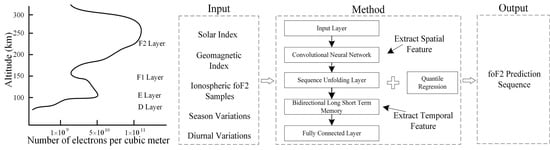
2.3. Hybrid Neural Network for Ionospheric Prediction

The hybrid neural network-based ionospheric foF2 prediction model is composed of a convolutional neural network, bidirectional long short-term memory network, and quantile regression mechanism. In contrast to traditional neural networks, CNN has two major characteristics in terms of local connection and weight sharing. The CNN network generally consists of the convolutional layer, and the core is the convolutional operation. With the advantages of convolutional operation, CNN can abstract and express the features of ionospheric variation.

In contrast to the traditional neural network, the recurrent neural network (RNN) network adds unit loops in the hidden layer to record historical information. The continuous partial derivative multiplications are produced when gradient descent is utilized for training the neural network. However, the long-term information indicates multiple iterations of the loops process. Therefore, the RNN network loses the ability to deal with time sequences due to its computation complexity. The LSTM is a special case of the RNN network. Compared with the neurons in RNN, the long short-term memory network’s neuron has several particular purpose nodes, such as input gate i, a forget gate f, an output gate o, and an internal memory unit c. The LSTM reduces the computation complexity encountered in RNN [19,20] via its unique structure. The obtained results are better than the time recurrent neural network and hidden Markov model. However, the LSTM is unable to encode back-to-front information encountered in time series. Therefore, the model is unable to obtain enough feature information [21,22], which causes the reduction in prediction accuracy. On the contrary, BiLSTM was proposed to solve this problem, indeed, it greatly reduced the prediction error.

The architecture of BiLSTM is implemented using MATLAB 2022a version deep learning toolboxes. Each of the unidirectional LSTMs is composed of forwarding and backward LSTM units. Similarly, the LSTM units are defined as:

$$f_t=\sigma \left(W_{xf}{x}_t+W_{hf}{h}_{t-1}+b_f\right),$$

(3)

$$i_t=\sigma \left(W_{xi}{x}_t+W_{hi}{h}_{t-1}+b_i\right),$$

(4)

$$c_t=f_t{c}_{t-1}+i_t\cdot tanh\left(W_{xc}{x}_t+W_{hc}{h}_{t-1}+b_c\right),$$

(5)

$$o_t=\sigma \left(W_{xo}{x}_t+W_{ho}{h}_{t-1}+b_o\right),$$

(6)

where $x_t$ is input vector to the LSTM unit; $\sigma$ represents sigmoid function; $W_{xf}$, $W_{xi}$, $W_{xc}$, $W_{xo}$, $W_{hf}$, $W_{hi}$, $W_{hc}$, and $W_{ho}$ are input and hidden weight matrices, respectively; $b_f$, $b_i$, $b_c$, and $b_o$ are bias vector parameters which need to be learned during training. The LSTM hidden layer ${\mathrm{h}}_t$ output is a function of output gate and memory cell with an activation function tanh, the hidden layer is defined as:

$$h_t=o_t\cdot \tanh \left(c_t\right),$$

(7)

where tanh is the activation function. Detailed description of the LSTM architecture is provided in [23,24].

The asymmetric distribution was worked out by the quantile regression [25,26,27], and it meticulously reflects the mapping information between inputs and response variables in a diverse range. Generally, the measurement samples of foF2 demonstrate characteristics of dynamic time-sequential and asymmetric distribution. Therefore, to enhance the prediction ability of the hybrid neural network on ionospheric foF2 sequence, we embed the QR mechanism in it. The $\tau$ quantile regression is defined as:

$$Q_{\tau }\left(\tau \right)=\underset{\gamma \in R}{\min }\left\{{\displaystyle \sum }_{i:Y_i\ge \gamma }\tau \left|Y_i-\gamma \right|+{\displaystyle \sum }_{i:Y_i\le \gamma }\left(1-\tau \right)\left|Y_i-\gamma \right|\right\},$$

(8)

The MSE function is generally utilized as the loss function in deep neural network regression layer. Here, we embed the QR and update it in the hybrid neural network architecture. According to Equation (8), the loss function is provided by:

$$Loss={{\displaystyle \sum }}_{i:Y_i\ge \gamma }\tau \left|Y_i-\gamma \right|+{{\displaystyle \sum }}_{i:Y_i\le \gamma }\left(1-\tau \right)\left|Y_i-\gamma \right|,$$

(9)

where $Y_i$ and $\gamma$ represent observed and predicted values, respectively.

Figure 2 depicts the architecture of the proposed hybrid neural network with quantile regression mechanism, consisting of the input layer, convolution layers, sequence unfolding layer, BiLSTM layer, quantile regression layer, fully connected layer, and output layer. Among them, the BiLSTM layer is composed of forwarding and backward LSTM units. The parameters of ionospheric foF2, UTs, UTc, DAYs, DAYc, F10.7, Dst, IMF-Bz, ap, and SSN are applied to the input layer. The process can be expressed as:

$$X^{foF2}=\left(UTs, UTc,DAYs,DAYc,Dst,IMF-Bz, ap,SSN,F10.7,foF2\right),$$

(10)

The output layer $Y_t^{foF2}$ combines the two layers, BiLSTM and CNN, with the quantile regression as:

$$Y_t^{foF2}=Concat\left(BiLST{M}_t^{output},CN{N}_t^{output}\right),$$

(11)

It is noted that the model performance is assessed through the root-mean-square error (RMSE), mean absolute error (MAE), and mean absolute percentage error (MAPE).

$$\mathrm{RMSE}=\sqrt{\frac{{{\displaystyle \sum }}_{i=1}^N{\left(U_i^{obs}-U_i^{model}\right)}^2}{N}},$$

(12)

$$\mathrm{MAE}=\frac{{{\displaystyle \sum }}_{i=1}^N\left|U_i^{obs}-U_i^{model}\right|}{N},$$

(13)

$$\mathrm{MAPE}=\frac{{{\displaystyle \sum }}_{i=1}^N\left|\frac{U_i^{obs}-U_i^{model}}{U_i^{obs}}\right|}{N},$$

(14)

where $U_i^{obs}$ indicates the foF2 measurement data, and $U_i^{model}$ is the model output.

3. Results

The program deploys that foF2 observations were acquired from 2009 to 2014. The total number of foF2 samples is split as 75% for training, and 12.5% for validation and testing/prediction, respectively. The proposed model performance is evaluated in four scenarios composed of low solar activity year (2010), high solar activity year (2014), and two geomagnetic storm events, as shown in

Table 1. The variation scenario on simulation conditions.

	Scenario 1	Scenario 2	Scenario 3	Scenario 4
Time	January–December 2010	January–December 2014	26 September 2011	15 July 2012
Geomagnetic Activity	--	--	Storm (<−30 nT)	Storm (<−30 nT)
Season	--	--	Spring	Winter
Solar Activity	Low	High	High	High

. The configurations of the models are presented in

Table 2. Model configurations of LSTM-foF2 and BiLSTM-foF2 ionospheric prediction model.

Model Configuration	LSTM-foF2	BiLSTM-foF2
Learning Method	Deep Learning	Deep Learning
Numbers of Hidden Unit 1	250	250
Numbers of Hidden Unit 2	250	250
Epoch	200	200
Minimum Batch Size	512	512

during scenario 1, and the rest of the scenarios are similar, as well. In addition, the weight of the quantile regression ($\tau$) is set to 0.75. For IRI-2016 model parameters, we used Sunspot number-R12, F-peak storm model (on), and the rest are maintained as default settings.

The performance of the proposed foF2 prediction model is evaluated under four scenarios, which contained quiet period and two space weather events. Here, we consider the seasons of spring (August, September, and October), summer (January, November, and December), autumn (February, March, and April), and winter (May, June, and July). In addition, we select one month of each season to evaluate model performance, and the detailed configuration is shown in

Table 3. Model configurations for 2010 and 2014.

Model Configuration		Summer	Autumn	Winter	Spring
Season	2010	January	March	June	September
	2014	January	March	June	September
Smooth monthly values of SSN	2010	14	18.5	24.6	29.5
	2014	109.3	114.3	114.1	101.9

.

3.1. Scenario 1: Analysis of Ionospheric foF2 Variation during Low Solar Activity Year (2010)

The solar cycle-24 began in December 2008 and ended in December 2019. The solar activity was minimal until 2010, but reached its maximum in 2014 with a smooth SSN monthly value of 81.8. The detailed variation of solar radiation flux F10.7 index in scenario 2 was depicted in Figure 3, and the measurement ionospheric foF2 sequence is utilized to evaluate models’ performance under low solar activity year. Here, we selected hourly foF2 for evaluation, and the measured data are compared with the results of the proposed method, the BiLSTM-based, the LSTM-based, and the IRI-2016 foF2 prediction model.

Figure 4 demonstrates the performance of test sample in different models. The LSTM network exhibits the highest prediction error, while the estimates of the proposed method are closer to the measured data.

The proposed model prediction results are compared with measured foF2 data and other models’ output under the different months presented in Figure 4. Figure 4a–l indicates the prediction foF2 results in one day under January (summer), March (autumn), June (winter), and September (spring), respectively. Considering the comparison of RMSE, MAE, and MAPE of whole months, the proposed method and other foF2 prediction models are summarized in

Table 4. Performance evaluation of prediction model for foF2 during January 2010.

Model Configuration (January)	RMSE (MHz)	MAE (MHz)	MAPE
IRI-2016	0.801	0.643	12.286%
LSTM-foF2	0.904	0.692	13.193%
BiLSTM-foF2	0.871	0.678	12.618%
Proposed method	0.77	0.60	11.802%

,

Table 5. Performance evaluation of prediction model for foF2 during March 2010.

Model Configuration (March)	RMSE (MHz)	MAE (MHz)	MAPE
IRI-2016	1.123	0.935	15.478%
LSTM-foF2	1.033	0.788	12.971%
BiLSTM-foF2	0.986	0.782	12.671%
Proposed method	0.878	0.701	12.468%

,

Table 6. Performance evaluation of prediction model for foF2 during June 2010.

Model Configuration (June)	RMSE (MHz)	MAE (MHz)	MAPE
IRI-2016	0.648	0.527	11.99%
LSTM-foF2	0.947	0.745	19.29%
BiLSTM-foF2	0.754	0.592	14.529%
Proposed method	0.583	0.46	10.24%

and

Table 7. Performance evaluation of prediction model for foF2 during September 2010.

Model Configuration (September)	RMSE (MHz)	MAE (MHz)	MAPE
IRI-2016	0.811	0.654	12.482%
LSTM-foF2	0.979	0.777	13.832%
BiLSTM-foF2	0.8	0.627	12.005%
Proposed method	0.688	0.542	10.608%

.

The results of the proposed method are well correlated with the measured data during the considered scenario, with RMSE values of 0.77, 0.878, 0.583, and 0.688 MHz. The proposed model has a noteworthy improvement compared with the LSTM-foF2 method during autumn (March) and spring (September). Similarly, the performance of proposed method has reduced with RMSE of 11.6%, 10.95%, 22.68%, and 14% during each month, respectively, compared with the BiLSTM-based foF2 prediction model. The response in MAPE is comparatively low with the proposed method compared with other foF2 prediction models. Similarly, the IRI-2016 and BiLSTM-foF2 models are fairly followed by the observed values but with further RMSE compared with the proposed method. The MAE and RMSE of the proposed method are lower than the other models, representing that the proposed method performed well during quiet periods.

3.2. Scenario 2: Analysis of Ionospheric foF2 Variation during High Solar Activity Year (2014)

In contrast to 2010, 2014 was one of the most active years in solar cycle-24, and the annual average sunspot number is counted at 113.3. Both the sunspot number and solar radiation flux F10.7 indicators can reflect solar activity, and the detailed variation of daily SSN was present in Figure 5. The solar flare is an important sign of activity, and it is a powerful burst of radiation. The sun welcomed 2014 with two mid-level flares on 31 December 2013 and 1 January 2014, and the severe solar flare (level-X1.6) event occurred on 17 September. To evaluate the ionospheric foF2 prediction models, we select the ionospheric foF2 measurement sequence during January, March, June, and September.

The proposed model prediction results compared with measured foF2 data and other models’ output under the different month are presented in Figure 6, and Figure 6a to Figure 6l depict one day for each month under spring (September), summer (January), autumn (March), and winter (June), respectively. Considering the comparison of RMSE, MAE, and MAPE of whole months, the proposed method and other foF2 prediction models are summarized in

Table 8. Performance evaluation of prediction model for foF2 during January 2014.

Model Configuration (January)	RMSE (MHz)	MAE (MHz)	MAPE
IRI-2016	1.05	0.851	10.26%
LSTM-foF2	1.03	0.812	9.763%
BiLSTM-foF2	0.959	0.767	9.52%
Proposed method	0.837	0.669	8.183%

,

Table 9. Performance evaluation of prediction model for foF2 during March 2014.

Model Configuration (March)	RMSE (MHz)	MAE (MHz)	MAPE
IRI-2016	1.582	1.451	15.442%
LSTM-foF2	1.816	1.527	15.812%
BiLSTM-foF2	1.808	1.577	16.106%
Proposed method	1.262	0.998	10.356%

,

Table 10. Performance evaluation of prediction model for foF2 during June 2014.

Model Configuration (June)	RMSE (MHz)	MAE (MHz)	MAPE
IRI-2016	1.163	0.96	16.99%
LSTM-foF2	1.42	1.104	22.656%
BiLSTM-foF2	1.16	0.945	17.643%
Proposed method	0.778	0.626	11.684%

and

Table 11. Performance evaluation of prediction model for foF2 during October 2014.

Model Configuration (October)	RMSE (MHz)	MAE (MHz)	MAPE
IRI-2016	1.281	1.054	14.667%
LSTM-foF2	1.134	0.911	12.847%
BiLSTM-foF2	1.06	0.844	11.961%
Proposed method	0.837	0.644	8.969%

.

The proposed method exhibits the lowest prediction error with an RMSE value of 0.778 MHz in June. On the contrary, the LSTM-foF2 model has poor results, with an RMSE value of 1.42 MHz. The response is relatively low with the LSTM-foF2 model compared with the measured samples, IRI-2016, and BiLSTM-based outputs. Similarly, the BiLSTM-foF2 model responds better when compared with IRI-2016 in winter (January) and spring (September), but their RMSE values are more when compared with the proposed method. The RMSE, MAE, and MAPE results indicate that the proposed method is well correlated with the measured samples on high solar activity year.

3.3. Prediction Analysis Results of Space Weather Events

Here, we evaluate the performance between the proposed method and other foF2 prediction models under two geomagnetic storm events that occurred in the period between 2011 and 2012. Scenario 3 to scenario 4, respectively, correspond to the storm events under different seasons.

3.3.1. Scenario 3: The foF2 Prediction Analysis for the 26 September 2011 Geomagnetic Storm

Several geomagnetic storm events occurred in 2011, among the unique intense storm developed on 26 September 2011. Figure 7 depicts scenario 3 of the proposed model and other model results with measured data during the storm event.

On 26 September 2011, the Dst value turned positive to negative at 17:00 h UT 26 September and lower than −30 nT, representing the storm’s beginning. It is noticed that the Dst value rapidly declined from 16:00 h UT [Figure 7b], and the maximum value of −118 nT was observed at 23:00 h UT. The above time indicates the crucial stage of the storms. A major part of the time from the 270th to 272nd days in 2011, was in the process of recovery from the storm event. The storms ended at 8:00 h UT on 30 September, and the Dst index completely recovered to normal. Significant deviations in foF2 were noticed on 26 September 2011 compared with the quiet periods, indicating the storm’s effects on ionospheric conditions. The observation sequence from 16:00 h UT 26 to 8:00 h UT 30 September was used to evaluate different ionospheric foF2 prediction models.

The prediction results of the proposed method and other models are shown in Figure 7a. Similarly, the RMSE values of the proposed method and other models considered in the comparison are summarized in

Table 12. Performance evaluation of prediction model for 26 September 2011 storm event.

Model Configuration	RMSE (MHZ)	MAE (MHZ)	MAPE
IRI-2016	1.059	0.865	13.5%
LSTM-foF2	1.373	1.017	14.86%
BiLSTM-foF2	1.035	0.814	11.587%
Proposed method	0.966	0.784	11.181%

. The proposed method predicted foF2 features with RMSE of 0.966 MHz, and the prediction values are followed with the measured data during the whole storm [Figure 7a]. In addition, the BiLSTM-foF2 model performed better when compared with the IRI-2016, but the RMSE is significantly more than the proposed method. It is evident from the results that the proposed method performed well during the considered storm event.

3.3.2. Scenario 4: The foF2 Prediction Analysis for the 15 July 2012 Geomagnetic Storm

Figure 8 depicts scenario 4 of the proposed model and other model results with measured data during the storm event of 15 July 2012. It is noticed that the storm took place in winter. On 15 July 2012, the Dst value turned positive to negative at 2:00 h UT, and a peak negative value of −139 nT was observed at 16:00 h UT on 15 July. The process indicated the main phase of the storm [Figure 8b]. The recovery phase of the storm begins at 19:00 h UT, and the Dst value had steadily risen [Figure 8b]. The end of the event is at 10:00 h UT on 18 July.

Evaluation of the different models’ performance is from 4:00 22 to 10:00 h UT 18 July during this storm event, and the prediction results of the proposed method and other models are shown in Figure 8b. Similarly, the RMSE, MAE, and MAPE of the proposed method and other models considered in the comparison are summarized in

Table 13. Performance evaluation of prediction model for 15 July 2012 storm event.

Model Configuration	RMSE (MHZ)	MAE (MHZ)	MAPE
IRI-2016	2.057	1.760	37.427%
LSTM-foF2	1.61	1.306	31.802%
BiLSTM-foF2	1.496	1.207	27.364%
Proposed method	1.265	0.996	22.737%

.

The predicted results of the proposed method are RMSE of 1.265 MHz, MAE of 0.996 MHz, and MAPE of 22.73%, respectively. It is clear from Figure 8a that the proposed method performed well during this storm event. Similarly, Table 13 reveals that the proposed method predicted well when compared with other models during this storm period. The error is relatively high with the LSTM-based model compared with BiLSTM-based and the proposed method. Similarly, the BiLSTM-foF2 model predicts better when compared with the IRI-2016 model, but their RMSE is significantly more compared with the proposed model.

4. Discussion

4.1. Analysis of Prediction Error Results

In this section, we calculate the samples error from different foF2 prediction models under low solar activity year (scenario 1), and the results are presented in Figure 9.

Figure 9d describes that the proposed method predicted well compared with the other models. The proposed model is performed well when the absolute error is less than 0.3 and 1.5 MHz. On the contrary, the LSTM-foF2 model has the worst correlation with measured samples. Similarly, the prediction errors are analyzed during the high solar activity year (scenario 2), as described in Figure 10.

Figure 10 elucidates the statistical and normal prediction error distribution. In addition, the proposed method presented in Figure 10d is crucially concentrated between −2 and 2 MHz, and the LSTM-based with the maximum error is between −4 and 4 MHz. Moreover, the LSTM-based, IRI-2016, BiLSTM-based, and proposed model predicted results have a maximum error of 1.816, 1.58, 1.808, and 1.262 MHz, respectively. The proposed method has a clear advantage compared with the above prediction models. Furthermore, Figure 10d reveals that the normal distribution curve of the proposed method is more well-fitted than the others, in which the normal distribution curve of the proposed model’s error is prominently concentrated. At the same time, the LSTM-based is scattered, indicating the improved performance of the proposed model compared with the other models. The MAE in the IRI-2016 model (0.851 MHz) and proposed model (0.626 MHz) reveals that the proposed method is well correlated with the measured samples under the high solar activity year.

Figure 11 shows the two storm events foF2 prediction error box plots for the different foF2 prediction models. The box represents the foF2 prediction errors for space weather events, in which the red signs represent outlier values. The top and bottom black bars represent the maximum and minimum values of the prediction error, respectively. The upper and lower edges of the blue box represent the upper and lower quartiles, respectively, in which the middle red represents the median. It is noticed that the proposed foF2 prediction model performed well when comparing the boxes.

4.2. Analysis of Quantile Regression Weight

Here, we further analyze the effect of quantile regression weight on the error of ionospheric foF2 prediction results. The month of February of the two solar years (2010 and 2014) was taken as an example for discussion. The weight is set to quartiles and deciles, and the configuration and prediction errors of the quartile’s weight during 2010 and 2014 are summarized in

Table 14. Prediction errors for quartiles during February 2010.

Quartiles Weight	RMSE (MHZ)	MAE (MHZ)	MAPE
0.25	1.33	1.11	17.65%
0.5	0.98	0.77	12.77%
0.75	0.86	0.67	11.95%

and

Table 15. Prediction errors for quartiles during February 2014.

Quartiles Weight	RMSE (MHZ)	MAE (MHZ)	MAPE
0.25	1.4	1.13	12.89%
0.5	1.21	0.96	10.85%
0.75	1.05	0.81	9.56%

.

Table 14 and Table 15 illustrate that the quantile weight in 0.75 has the smallest RMSE, MAE, and MAPE error in the case of quartiles during 2010 and 2014. In addition, the deciles are utilized to further discuss the prediction results. The RMSE values of prediction results under the different solar activity years are presented in Figure 12, and the detailed value is summarized in

Table 16. The division of foF2 samples.

Input Time Series Length	Training Samples (Input)	Validation Samples	Test/Predict Samples (Output)
One month	December 2009	January 2010	February 2010
Three months	October–December 2009	January 2010	February 2010
Six months	July–December 2009	January 2010	February 2010
Nine months	April–December 2009	January 2010	February 2010
Full	January–December 2009	January 2010	February 2010

.

The quantile weight in 0.1 has a maximum RMSE value of 1.66 MHz and a minimum of 0.86 MHz in 0.75 during 2010. Similarly, the maximum and minimum RMSE values of 1.73 and 1.05 MHz are produced in quantile weights of 0.1 and 0.75, respectively, in 2014. In addition, Figure 12 describes that the ionospheric foF2 prediction error has significantly declined from a quantile weight of 0.2, and the foF2-RMSE value curve is relatively stable from a quantile weight of 0.6 to 0.8.

4.3. Analysis of Input and Output foF2 Time Series Length

In this section, we evaluate the limited time series input and different lengths of output for the ionospheric foF2 prediction model. The total foF2 samples are set from January 2009 to February 2010, and the division is presented in Table 16. We use hourly foF2 samples and set the complete training samples to include data from January to December 2009. Similarly, validation samples and test samples are set to January and February 2010, respectively. To analyze the limited time series, we set the input time lengths as one, three, six, and nine months, and the prediction results are presented in

Table 17. Prediction error analyses for different time series lengths.

Input Time Series Length	RMSE (MHZ)	MAE (MHZ)	MAPE
One month	1.80	1.54	24.52%
Three months	1.49	1.23	19.84%
Six months	1.14	0.87	14.28%
Nine months	0.93	0.73	12.2%
Full	0.86	0.67	11.95%

.

It is clear from Table 17 that the complete training samples perform better than the other conditions. Generally, diurnal and seasonal variations are significant features of ionospheric foF2. With the input short time series, deep learning is hard to learn and capture features of foF2 variation. In addition, since deep learning-based ionospheric foF2 prediction models need sufficient training samples to learn features between input elements, we consider that input length (training samples) should include nine months (three seasons) at least to obtain better prediction performance (RMSE less than 1 MHz) for the input limited time series length.

In addition, the different lengths of outputs are analyzed. The total foF2 samples are consistent with the above, and we set training samples from January to December 2009, and validation samples are set for January 2010. A detailed explanation of the foF2 sample division is shown in

Table 18. The setting for output time series length.

Output Time Series Length	Training Samples (Input)	Validation Samples	Test/Predict Samples (Output)
One month	January–December 2009	January 2010	February 2010
Three months	January–December 2009	January 2010	February–April 2010
Six months	January–December 2009	January 2010	February–July 2010
Nine months	January–December 2009	January 2010	February–October 2010
Twelve months	January–December 2009	January 2010	February 2010–January 2011

. For the test/prediction set, we set one, three, six, nine, and twelve months to analyze performance, and the prediction results are presented in

Table 19. Prediction error analyses for different time series output lengths.

Output Time Series Length	RMSE (MHZ)	MAE (MHZ)	MAPE
One month	0.86	0.67	11.95%
Three months	0.88	0.68	13.16%
Six months	0.92	0.7	14.81%
Nine months	0.93	0.72	15.9%
Twelve months	1	0.79	16.05%

.

It is evident from Table 19 that the one-month condition performs better than others. The prediction performance in twelve months is the worst when compared with other conditions. In addition, the RMSE values are relatively stable from three-to-nine-month conditions.

5. Conclusions

This paper proposes a hybrid neural network with quantile regression mechanism, to predict the ionospheric foF2 variation over the low latitude region. The model input parameter (foF2) is considered from the ionosonde located at the Brisbane station (27°53′S, 152°92′E) along with space weather parameters F10.7, SSN, IMF-Bz, ap, and Dst from 2009 to 2014. We design four scenarios (high and low solar activity year and two space weather events) and use measured foF2 data to evaluate the performance of the proposed model. The prediction results are compared with IRI-2016, LSTM-based, and BiLSTM-based models’ output values. In addition, we further analyzed and discussed the performance of different models in the considered storm scenarios (26 September 2011 and 15 July 2012). The RMSE, MAPE, MAE, and statistical error analysis demonstrate that the proposed model strikes a favorable performance compared with the other previous models during the high and low solar activity and geomagnetic storm periods.

The ionospheric foF2 determines the working frequency of the shortwave signal, and an accurate frequency prediction can reduce the complexity of frequency selection. In summary, the proposed model is ideally suited to predict the variations of ionospheric parameters, and the results are helpful in frequency selection and global navigation satellite system position. Future studies will constantly test the proposed model in foF2 measured data from other ionospheric observatories over low latitude regions, and discuss optimal space weather parameters for the deep network model’s input during space weather events.

References

1. Bilitza, D.; Obrou, O.; Adeniyi, J.; Oladipo, O. Variability of foF2 in the equatorial ionosphere. Adv. Space Res. 2004, 34, 1901–1906. [Google Scholar] [CrossRef]
2. Oyeyemi, E.O.; McKinnell, L.A.; Poole, A.W.V. Near-real time foF2 predictions using neural networks. J. Atmos. Sol. Terr. Phys. 2006, 68, 1807–1818. [Google Scholar] [CrossRef]
3. Bai, H.; Feng, F.; Wang, J. A Combination Prediction Model of Long-Term Ionospheric foF2 Based on Entropy Weight Method. Entropy 2020, 22, 442. [Google Scholar] [CrossRef] [PubMed] [Green Version]
4. Chen, C.; Wu, Z.S.; Xu, Z.W.; Sun, S.J.; Ding, Z.H.; Ban, P.P. Forecasting the local ionospheric foF2 parameter 1 hour ahead during disturbed geomagnetic conditions. J. Geophys. Res. Space Phys. 2010, 115, 135–146. [Google Scholar] [CrossRef]
5. Olga, M. The Influence of Space Weather on the Relationship Between the Parameters TEC and foF2 of the Ionosphere. IEEE J. Radio Freq. Identif. 2021, 5, 261–268. [Google Scholar]
6. Sun, W.; Long, X.; Xin, H. Forecasting of ionospheric vertical total electron content (TEC) using LSTM networks. In Proceedings of the 2017 International Conference on Machine Learning and Cybernetics (ICMLC), Ningbo, China, 9–12 July 2017 . [Google Scholar]
7. Suin, M.; Yong, H.K.; Jeong, H.; Young, K.; Jong, Y. Forecasting the Ionospheric F2 Parameters over Jeju Station (33.43°N, 126.30°E) by Using Long Short-Term Memory. J. Korean Phys. Soc. 2020, 77, 1265–1273. [Google Scholar]
8. Li, X.J.; Zhou, C.; Tang, Q.; Zhao, J.; Zhang, F.B.; Xia, G.C.; Liu, Y. Forecasting Ionospheric foF2 Based on Deep Learning Method. Remote Sensing 2021, 13, 3849. [Google Scholar] [CrossRef]
9. Kim, J.H.; Kwak, Y.S.; Kim, Y.H.; Moon, S.I.; Jeong, S.H.; Yun, J.Y. Potential of Regional Ionosphere Prediction Using a Long Short-Term Memory Deep-Learning Algorithm Specialized for Geomagnetic Storm Period. Space Weather 2021, 19, 1–20. [Google Scholar] [CrossRef]
10. Rao, T.V.; Sridhar, M.; Ratnam, D.V.; Harsha, P.B.S.; Srivani, I.A. Bidirectional Long Short-Term Memory-Based Ionospheric foF2 and hmF2 Models for a Single Station in the Low Latitude Region. IEEE Geosci. Remote Sens. Lett. 2021, 19, 1–5. [Google Scholar] [CrossRef]
11. Williscroft, L.A.; Poole, A.W. Neural networks, foF2, sunspot number and magnetic activity. Geophys. Res. Lett. 1996, 23, 3659–3662. [Google Scholar] [CrossRef]
12. McKinnell, L.A.; Poole, A.W.V. Ionospheric variability and electron density profile studies with neural networks. Adv. Space Res. 2001, 27, 83–90. [Google Scholar] [CrossRef]
13. Athieno, R.; Jayachandran, P.T.; Themens, D.R. A neural network based foF2 model for a single station in the polar cap. Radio Sci. 2017, 52, 784–796. [Google Scholar] [CrossRef]
14. Perna, L.; Pezzopane, M. foF2 vs solar indices for the Rome station: Looking for the best general relation which is able to describe the anomalous minimum between cycles 23 and 24. J. Atmos. Sol. Terr. Phys. 2016, 148, 13–21. [Google Scholar] [CrossRef] [Green Version]
15. Joshua, E.O.; Nzekwe, N.M. foF2 correlation studies with solar and geomagnetic indices for two equatorial stations. J. Atmos. Sol. Terr. Phys. 2012, 80, 312–322. [Google Scholar] [CrossRef]
16. Kane, R.P. Solar cycle variation of foF2. J. Atmos. Sol. Terr. Phys. 1994, 54, 1201–1205. [Google Scholar] [CrossRef]
17. Bai, H.M.; Feng, F.; Jian, W.; Wu, T.S. Nonlinear dependence study of ionospheric F2 layer critical frequency with respect to the solar activity indices using the mutual information method. Adv. Space Res. 2019, 5, 1085–1092. [Google Scholar] [CrossRef]
18. Campbell, W.H. Occurrence of AE and Dst geomagnetic index levels and the selection of the quietest days in a year. J. Geophys. Res. 1979, 84, 75–881. [Google Scholar]
19. Ergen, T.; Kozat, S.S. Online Training of LSTM Networks in Distributed Systems for Variable Length Data Sequences. IEEE Trans. Neural. Netw. Learn. Syst. 2018, 29, 5159–5165. [Google Scholar] [CrossRef] [Green Version]
20. Sherstinsky, A. Fundamentals of recurrent neural network (RNN) and long short-term memory (LSTM) network. Phys. D Nonlinear Phenom. 2020, 404, 132306. [Google Scholar] [CrossRef] [Green Version]
21. Mustaqeem Sajjad, M.; Kwon, S. Clustering-Based Speech Emotion Recognition by Incorporating Learned Features and Deep BiLSTM. IEEE Access 2020, 8, 79861–79875. [Google Scholar] [CrossRef]
22. Siami-Namini, S.; Tavakoli, N.; Namin, A.S. The performance of LSTM and BiLSTM in forecasting time series. In Proceedings of the 2019 IEEE International Conference on Big Data (Big Data), Los Angeles, CA, USA, 9 September 2019; IEEE: Piscataway, NJ, USA, 2019; pp. 3285–3292. [Google Scholar]
23. Kumar, S.D.; Subha, D. Prediction of Depression from EEG Signal Using Long Short Term Memory (LSTM). In Proceedings of the 2019 3rd International Conference on Trends in Electronics and Informatics (ICOEI), Tirunelveli, India, 23–25 April 2019; IEEE: Piscataway, NJ, USA, 2019; pp. 1248–1253. [Google Scholar]
24. Zhang, X.; Zhang, Y.; Lu, X.; Bai, L.; Chen, L.; Tao, J.; Wang, Z.; Zhu, L. Estimation of Lower-Stratosphere-to-Troposphere Ozone Profile Using Long Short-Term Memory (LSTM). Remote Sens. 2021, 13, 1374. [Google Scholar] [CrossRef]
25. Koenker, R.; Hallock, K. Quantile Regression-An introduction. J. Econ. Perspect. 2000, 15, 143–156. [Google Scholar] [CrossRef]
26. Zhang, W.; Quan, H.; Gandhi, O.; Rajagopal, R.; Tan, C.; Srinivasan, D. Improving Probabilistic Load Forecasting Using Quantile Regression NN With Skip Connections. IEEE Trans. Smart Grid. 2020, 11, 5442–5450. [Google Scholar] [CrossRef]
27. Taylor, W. A Quantile Regression Neural Network Approach to Estimating the Conditional Density of Multiperiod Returns. J. Forecastin. 2020, 19, 299–311. [Google Scholar] [CrossRef]
Figure 1. Variation of (a) geomagnetic index, Dst; (b) geomagnetic index, ap; (c) foF2 measurement samples; (d) solar activity index, F10.7.
Remotesensing 14 05418 g001aRemotesensing 14 05418 g001b
Figure 2. The hybrid neural network foF2 prediction architecture.
Remotesensing 14 05418 g002
Figure 3. The variation of F10.7 index during 2010.
Remotesensing 14 05418 g003
Figure 4. (al) The proposed foF2 prediction model results comparison during 2010.
Remotesensing 14 05418 g004
Figure 5. The variation of SSN during 2014.
Remotesensing 14 05418 g005
Figure 6. (al) The proposed foF2 prediction model results comparison during 2014.
Remotesensing 14 05418 g006
Figure 7. Variations of foF2 (a), Dst (b), and ap (c) during the 26 September 2011 geomagnetic storm.
Remotesensing 14 05418 g007
Figure 8. Variations of foF2 (a), Dst (b), and ap (c) during the 14 July 2012 geomagnetic storm.
Remotesensing 14 05418 g008aRemotesensing 14 05418 g008b
Figure 9. Comparison of cumulative distribution of prediction errors: (a) LSTM-foF2; (b) BiLSTM-foF2; (c) IRI-2016; (d) proposed model.
Remotesensing 14 05418 g009
Figure 10. Histograms and the normal distribution curve of the prediction errors: (a) LSTM-foF2; (b) BiLSTM-foF2; (c) IRI-2016; (d) proposed model.
Remotesensing 14 05418 g010
Figure 11. Statistical prediction error analyses for different prediction models.
Remotesensing 14 05418 g011
Figure 12. Prediction error analyses for deciles quantile regression weight: (a) February 2010 and (b) February 2014.
Remotesensing 14 05418 g012