1. Introduction
Accurately estimating the position and orientation of a robot indoors is a challenge usually solved by Simultaneous Localization and Mapping (SLAM) technologies [
1]. A robot uses SLAM to locate itself according to the map and its own sensors during movement and constantly builds incremental maps. Recent years have witnessed a growing interest in SLAM due to its wide application in 3D reconstruction, augmented reality (AR), virtual reality (VR), and autonomous driving. Benefiting from the improvement and popularization of optical camera technology, visual SLAM has become a popular research field. Compared with a complete visual SLAM pipeline, visual odometry (VO) uses a series of images to estimate the camera’s pose in real time and robot trajectories often drift over time [
2].
VO algorithms can be categorized into feature-based methods, direct methods, and semi-direct methods (which combine the former two). Feature-based methods extract image features, calculate feature descriptors for frame matching, and discard most of the image information [
3]. Direct methods estimate the camera motion by minimizing the photometric error between consecutive frames, making full use of all photometric information on the image [
4,
5]. Semi-direct methods detect the features on the image and estimate the camera motion using the photometric information of the features [
6,
7]. All VO algorithms locate themselves by tracking the stable environment around them during camera movement. Therefore, because VO algorithms cannot distinguish between stationary objects and moving objects, they fail if there are moving obstacles around. In the indoor environment, the interference created by surrounding moving obstacles can be addressed by using ceiling-view VO (CV-VO) methods [
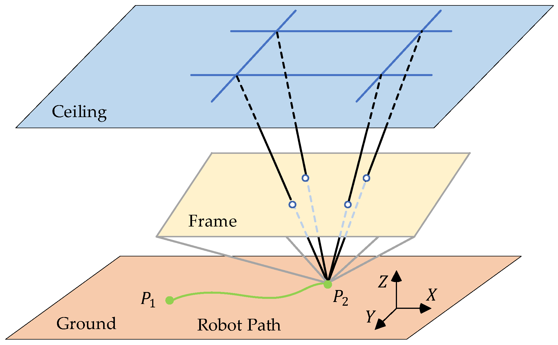
8]. The ceiling image has the advantages of being static, rarely occluded, and well-structured. As shown in
Figure 1, the camera in ceiling-view VO methods moves on the ground and the trajectory is approximately parallel to the ceiling, which means the problem of pure rotation failure can also be avoided. However, compared with the image captured by the forward-looking camera, the ceiling image captured by the upward-looking camera has more repetitive patterns and often has fewer features. Therefore, extracting as much information as possible from limited observations becomes the key to the ceiling-view VO method.
Various SLAM methods involve extracting image point features [
3,
9] and have achieved good results in most scenes. In low-textured environments, point features cannot provide sufficient information and the performance of the above-mentioned methods usually reduces. In such instances, line features are taken as additional constraints and these point line systems show better results in low-textured environments [
10,
11]. However, due to the difficulty in matching line features (partial occlusion, line disconnection, unstable endpoint extraction), the trajectory estimation is still not stable [
12,
13]. Apart from line features, the indoor environment also has structured information. Indoor walls and ceilings can provide point features and line features for positioning, and the distribution of these features includes orthogonal, coplanar, and other geometric relationships. This structured information can be used to estimate the robot pose [
14]. The structured information in the indoor environment has been exploited in the indoor visual SLAM system to improve stability and accuracy [
15,
16]. Due to the limited field of vision in the direction of observation, the ceiling–view VO method cannot obtain sufficient structural information of indoor scenes, including information related to floors, walls, and ceilings, unlike the front-view VO method. When only the ceiling plane can be stably observed, it also helps extract the coplanar structural information in the ceiling, which can be used to reduce the positioning error. Indoor ceilings (such as ceilings of corridors, garages, and restaurants) often have obvious repetitive artificial structures, containing rich line features, which are all subject to the coplanar constraint of the ceiling plane.
On the basis of the above ideas, in this work, we try to exploit structural constraints in semi-direct visual odometry in the ceiling scene with repetitive line features. We describe in detail the combination, including pose estimation with additional plane constraints and joint optimization of geometric constraints and photometric errors. Since there is no open-source dataset for the evaluation of ceiling-view VO methods (CV-VO), we propose a new ceiling dataset to fill this research gap to some extent.
The experimental platform for collecting the ceiling dataset was equipped with an upward-looking camera, an inertial measurement unit (IMU), and rotary light detection and ranging (LiDAR). We collected ceiling image data from different scenes in the office area, the building hall, and the underground parking lot. During data collection, we recorded the data of all sensors at the same time, among which IMU and high-precision LiDAR data were used to produce the ground truth of the trajectory. We conducted experiments on the dataset, and results showed that by combining the structural regularities of plane constraints, our method achieves better performance in the ceiling scene with repetitive lines.
In summary, the main contributions of our work are in the following two aspects:
We integrate structural constraints seamlessly with the semi-direct method framework, named Struct-PL-SVO. The proposed method is applicable to the ceiling-view VO system, while requiring a low level of computation. It estimates camera pose through coplanar constraint of point line features. In the sliding window optimization process, geometric constraint and photometric error are simultaneously used and optimization is performed on multiple keyframes to refine the depth of features and the camera pose. To ensure the reproducibility of all our results and benefit the robot community, relevant codes are made available online (
https://github.com/githubwys/Struct-PL-SVO, accessed on 20 August 2022).
To evaluate the performance of the ceiling-view VO method, we propose a visual dataset of ceiling scenes. The dataset is collected from the wheeled robot platform and contains ceiling scenes in different patterns (office area, building hall, underground parking lot). The upward-looking camera captures the ceiling image data, and the LiDAR-Inertial SLAM method generates the ground truth of the pose with high accuracy. The dataset is available online (
https://github.com/githubwys/Struct-PL-SVO, accessed on 20 August 2022).
2. Related Work
2.1. Taxonomy of Visual Motion Estimation Methods
The methods of recovering the camera pose from video can be classified into three categories: feature-based methods, direct methods, and semi-direct methods. Feature-based SLAM estimates the robot’s pose by extracting image features, calculating and matching feature descriptors, tracking features along consecutive frames, and later minimizing some error functions (usually based on reprojection errors) [
17]. These methods perform well in a richly textured environment but fail easily due to feature matching errors in the case of repeated features. In addition, feature descriptors and matching features involve high levels of computation. The direct method directly estimates the structure and motion from the intensity value in the image, which has better stability when the environment has less texture [
18] and there is motion blur [
19], but it is sensitive to photometric changes. The semi-direct method extracts features and uses the photometric information of the features instead of feature descriptors to estimate the position and pose. Thus, the feature tracking remains stable even when the feature descriptors are similar [
6,
7].
The ceiling image usually has relatively few features, the texture is repetitive, and the image structure is simple. Therefore, the ceiling-view VO method needs to obtain as much information as possible from such repetitive and few features. Feature-based methods may fail due to feature matching errors. However, the direct method and semi-direct method based on photometric information do not depend on feature descriptor matching, so they still have good performance in repetitive texture environment. In addition, these methods do not involve calculating feature descriptors and carrying out the calculation of feature matching, making them faster than feature-based methods [
4,
6].
2.2. Structure Constraints Methods
The method based on point features has achieved good performance in texture-rich scenes. ORB-SLAM relies on fast and continuous tracking of ORB features [
20] and local optimization with continuous observation of point features. However, in low-textured scenarios, the methods based on point features have reduced accuracy and sometimes even fail because it is difficult to find enough key point features. The structural regulation of the artificial environment is expressed by the line features in the environment. Thus, many methods that optimize the camera pose by taking the line features as a supplement to the point features have been proposed [
10,
11]. The improved semi-direct method PL-SVO introduces line features as additional constraints [
7]. However, the extraction of line features is unstable because a change in endpoints makes it difficult to match and track line features. Moreover, in ceiling scenes, there are fewer point features and more repetitions, which leads to more fuzziness in methods based on point and line features. In [
21], it is shown that the adoption of line features in SLAM systems sometimes worsens performance compared to SLAM systems that use only point features.
In addition to line features, the indoor artificial environment also has structured information, such as orthogonal and coplanar features [
14]. The Manhattan hypothesis is used to improve the feature-based method [
15,
16]. Methods using direction information and structural lines as feature constraints are proposed in [
21]. In the indoor environment, the ceiling has a strong coplanar constraint, which can provide effective structured information for ceiling-view VO methods.
2.3. Ceiling-View Visual Odometry Methods
One of the seminal work on ceiling vision is the ceiling mosaic method [
22], in which particle filter localization was adopted by comparing the ceiling mosaic map and the current visual observation. The other representative approaches usually extract corner points as features. CV-SLAM based on monocular upward-looking camera builds maps by detecting corner points [
8,
23] and uses the extended Kalman filter (EKF) to estimate the robot pose, which leads to good results in an environment with non-repetitive features. Some ceiling VO methods achieve positioning by detecting lights, doors, and corners as visual features [
24,
25]. Visual node descriptors and map updating methods that are not affected by ceiling patterns were proposed in [
26].
The indoor ceiling often contains many line features, which are not easily affected by changes in light and the angle of view and can improve the stability of the VO system. The improved method of CV-SLAM uses point and line features to build a more complete map [
27]. For a ceiling scene with rich line features, the main direction method is proposed, which uses the RGB-D camera to obtain point clouds for matching to estimate the camera pose [
28]. The current ceiling-view VO methods use the point and line features of the ceiling but do not use the structural information of the indoor environment. According to the characteristics of the ceiling, it is logical to use the coplanar structural constraint to expand the VO method. However, as far as we know, there is no semi-direct VO system using structural constraints. We are the first to establish such a pipeline and use it in the ceiling scene.
3. System Overview
Our method introduces coplanar structured constraints into the semi-direct method. To improve the accuracy of the system, we use the coplanar constraint of point line features to estimate the pose. The coplanar constraint is also added in the sliding window optimization module, together with the photometric error, to improve the final positioning result.
As shown in
Figure 2, the system is mainly composed of two components: visual odometry and sliding window optimization. The visual odometry module estimates the camera motion between frames, and the sliding window optimization module optimizes the local feature map. First, the system receives the image and sends it to the visual odometry module, calculates the initial value of the relative pose of the adjacent frames using the sparse model image alignment method, and then uses the feature alignment method to optimize the position of the features on the current frame. After that, the system transfers the image to the backend, sliding the window optimization module, and determines through the keyframe selection strategy whether the current frame is a keyframe. If the current frame is not a keyframe, the depth filter is iterated using the frame. When the iteration reaches the convergence condition, the feature is inserted into the feature map. The keyframe is added to the keyframe sequence of the current local map, and the common plane in the space is extracted. Subsequently, the photometric error and the geometric constraint of the plane are used to optimize the position of features. For keyframes, we need to detect new features and establish and initialize the depth filters.
In the remaining sections, we will describe the composition in detail.
4. Visual Odometry with the Coplanar Constraint
The observation scene of the ceiling-view VO methods is the ceiling. Most of the features in the image are on the ceiling plane, and the lines and points on the plane conform to the coplanar constraint. Therefore, in this paper, we extract and use the coplanar constraint between features to solve the translation between camera frames.
4.1. Identification of Coplanar Feature Sets
A plane imaged by two cameras induces a homography H on the image points in the two cameras. Because of the above constraints, the coplanar points and coplanar lines between the two frames can be confirmed by calculating characteristic lines [
14,
15].
First, the point and line features in the current frame are obtained by Sparse-Model-based Image Alignment and Relaxation Through Feature Alignment [
7], both based on minimizing photometric error between frames rather than feature detection. Then, the 3D lines corresponding to line features are classified. The parallel 3D lines are recorded as a line cluster S, and the set of all line clusters is {S}. All the 3D lines in S are parallel to each other but not necessarily coplanar. We get the coplanar line set {C} from {S} by the “characteristic line” (CL) [
14], which is an invariant representation of coplanar and parallel 3D lines. Specifically, if a set of 3D lines are parallel and on the same plane, their corresponding 2D lines share a common CL. That is, a set of coplanar lines marked as C correspond to their own CL, as shown in
Figure 3. By exploiting different CLs, we can obtain the final {C} from all 3D lines {S}. Furthermore, some sets C from {C} are merged if they meet the same homography matrix, which means they are coplanar.
We can identify all coplanar 3D lines and the homography matrix. In the end, if the 2D point matches projected by a 3D point on two images conform to the homography matrix constraint, the corresponding 3D point belongs to the coplanar points.
4.2. Translation Optimized by Coplanar Features
After confirming all coplanar space lines and coplanar space points, we can build a model that can unify coplanar point features and coplanar line features to solve the translation between the two frames.
The homography matrix
of the same plane on two images can be decomposed into [
29]:
We bring the initialized , which represents the rotation matrix between two frames, into Equation (1). In addition, represents the vertical distance from the camera projection center to the spatial plane, represents the normal vector of the space plane in the camera coordinate system, and represents the translation between two frames that we need to estimate.
S denotes a space straight line, and
are the plane straight lines projected in the
i-th frame and the
j-th frame, respectively, as shown in
Figure 4. Any corresponding points on two straight lines
and
satisfy the constraint of homography matrix:
By bringing Equation (2) into Equation (1), we can obtain the following equation:
Similarly, the space point
is projected on the plane in the two frames marked as points
and
, which are constrained by the homography matrix of coplanar points:
Thus, the following equation can also be deduced:
Coplanar points and lines can provide the same form of linear equation, so we can use a unified model to solve . For all coplanar points and coplanar lines, we can obtain an overdetermined linear equation about , which can be solved by the least square method. To solve the equation, we need the depth from the i-th frame to the plane , which can be provided in the sliding window optimization module.
When the translation is obtained, we put as a fixed value and resolve the variable R in the relative pose T of the consecutive frame. At this time, in the six dimensions of the relative pose T, the translation is known and R can be solved by the iterative method that minimizes photometric errors.
In the visual odometry module, we estimate the relative pose T between consecutive frames by using coplanar feature constraints and the homography matrix.
5. Sliding Window Optimization with the Coplanar Constraint
To improve the optimization accuracy and ensure speed, we maintain a local feature map containing only part of the keyframes in the sliding window optimization part. In this paper, the plane of coplanar features is extracted in the sliding window optimization module. After that, the photometric error and the coplanar constraint are used to optimize the features and the keyframes.
5.1. Keyframe Selection
The new frame is selected as the keyframe if the Euclidean distance between the new frame and all keyframes exceeds 10% of the average scene depth. When a new keyframe is inserted, the keyframe farthest from the current camera position will be removed. Therefore, the number of keyframes in the local map remains unchanged, ensuring efficiency. All point features and line features that cannot be projected into the existing local map keyframes will also be removed.
If the current frame is a keyframe, the point and line features are extracted by FAST detection and LSD segments detection and the detected features are used to initialize new depth filters. The space plane is extracted from the feature map to optimize the feature map and keyframes. If the current frame is not a keyframe, we use the current frame to iterate the depth filter. The feature will be inserted into the feature map when the feature’s depth filter iteration meets the convergence conditions.
5.2. Estimating the Plane of Coplanar Features by Linear Regression
In the indoor environment, the upward-looking method completes its positioning by observing the ceiling. To use the coplanar constraint of the ceiling, it is necessary to extract the ceiling plane from the feature map first. When the current frame is set as the keyframe, we detect whether all the point features and line features in the world coordinate system are coplanar in the feature map and extract the plane of the coplanar features. To parameterize the ceiling plane
of the coplanar features, we use the Hesse form:
In the equation, represents the normalized normal vector of the plane and is the distance from the plane to the coordinate system origin.
When estimating the ceiling plane of the coplanar features, we have N given feature points in the feature map and obtain the plane with the smallest average point plane distance of these N points.
Because the feature points on the wall interfere, we use the RANSAC method to estimate the ceiling plane and take the sum of the distance from the feature to the plane as the error function to identify the optimal plane
. Thus, the sum of the distances D from the given N coplanar feature points to the plane is the smallest. Theoretically, the distance between the coplanar feature points and the plane is 0. However, the spatial coordinates of the feature point obtained by the depth have random errors and thus the distance between the coplanar points and the plane is not 0. We assume that the error is Gaussian distribution with 0-means. For a point
in space, the distance
to the plane
is:
Because the formula of distance between points and surfaces is a linear term about plane parameters. Moreover, the noise error is assumed to satisfy the Gaussian distribution. Therefore, the plane fitting problem can be transformed into a multiple linear regression problem, as follows:
Placing the coplanar feature points in the feature map into Equation (9), we obtain:
In the equation, matrix
is
.
means
, and it represents the world coordinates of the i-th feature point, which participates in the calculation of the plane parameters.
and
, and these parameters can be solved by the least square method:
After the parameter W is calculated, d can be solved according to the characteristic that n is the unit normal vector and the module length is 1. So far, all the parameters of the plane have been ascertained.
5.3. Plane Update
When adding a new keyframe, we detect the coplanarity of all spatial features newly added to the feature map. We first determine whether these new features are located on the plane in the feature map. For the point feature, the distance between the point and the plane should be 0 because the point is located on the plane .
Taking into account the error of the depth filter iteration depth to calculate the spatial coordinates, we empirically set the threshold to
. If the distance between the point and the plane is less than three times the MSE of the plane fitting in the previous stage, the point is considered to be on the plane, as shown in
Figure 5.
For the line feature, if its two endpoints are on the plane, we assume that the line feature is on the plane.
We regard the space points within the error range as points on the plane and record them as inner points. The space points outside the error range are recorded as outer points. After filtering out the inner points in the feature map, we use the inner points to fit the feature plane again as the final feature plane.
5.4. Optimization with Both the Geometric Constraint of Coplanarity and the Photometric Error
After fitting the spatial plane of the ceiling in the local feature map, we optimize the coordinates of all inner points with the photometric error and geometric constraints.
To obtain new geometric constraints for the positions of coplanar feature points, we extract the spatial plane. To calculate the depth d, the feature points in the feature map use the depth filter, thereby obtaining the spatial coordinates of the feature. This process uses only photometric information. After obtaining the geometric constraints, we use a new method to simultaneously exploit the geometric information and the photometric information. At this time, the coordinates of the spatial feature points should meet two conditions: (1) Photometric error constraint: The average reprojection error from spatial feature points to each keyframe should be minimized. (2) Geometric constraint of coplanarity: The distance from the spatial feature point to the common plane should be less than the tolerance.
The space feature points extracted from keyframe
are marked as
, and the feature point 2D coordinate of the keyframe
is marked as
(the photometric calculation based on feature-patches) [
6]. The depth of space feature points
relative to the keyframe
is
. The feature points
are projected on other keyframes
, recorded as
. To minimize the photometric error of the projection, we make the space feature points
move along the direction of their depth
. The motion range
is maintained within
. As shown in
Figure 6, the equation can be expressed as:
where
is the set of all keyframes in the local feature map. Through the movement of feature points within the range of geometric constraints, we identify the optimal depth to minimize the photometric error of feature points on the keyframes and other keyframes, while satisfying geometric constraints.
For the line feature, the two endpoints of the line feature are optimized by the same method as that used for the point feature to complete photometric error and plane constraint.
5.5. Initialization of the Depth Filter by the Plane
The semi-direct method uses the depth filter to filter and calculate the depth value of candidate feature points. According to the mean value 𝜇 and the variance 𝜎 of the current feature point in the depth filter, the system finds the corresponding epipolar line in the current frame and searches for matching pixel blocks with similar grayscales on the epipolar line. The mean value 𝜇 of Gaussian distribution represents the feature inverse depth, which determines the search position on the epipolar line. Variance 𝜎 represents the uncertainty of feature inverse depth and determines the range of search. However, this method is limited by the initial value of the depth filter. The convergence result and the convergence speed of the mean value of the depth filter are closely related to the initial value.
If the initial value is not appropriate, it is difficult to converge to the best position and the convergence speed slows down.
The upward-looking camera observes the ceiling, which ensures that most of the features are located on the same plane. Therefore, we can use this property to predict the initial depth of the features and provide the initial value of the depth for the depth filter. The parameter of the ceiling plane
in the world coordinate system is
, and the pose of the current frame is
. In addition, the plane parameter of the plane in the current frame is marked as
:
The coordinate of the feature point in the camera coordinate system of the current frame is
, and the depth on the current frame is
. The coordinate of the feature under the current frame
. According to the equation of the point surface distance:
After solving the coordinate X of the feature in the current frame, we can estimate the depth of the feature. By taking the reciprocal of the estimated depth value as the initial value of the mean value 𝜇, we can prevent the matching failure due to the excessive deviation of the epipolar line search position. Meanwhile, the calculated depth value is also the parameter required in the visual odometry module.
6. Ceiling Dataset
The ceiling scene is the target scene of the proposed method. However, there is no open-source ceiling visual dataset. To evaluate the effectiveness of the algorithm in our paper, we present a dataset of the ceiling scene for the ceiling visual-based VO method. As far as we know, we are the first to establish and publish such a ceiling dataset, making up for the lack of data in this research field and the difficulties in evaluation.
6.1. Hardware Device
To collect RGB images of the ceiling, this dataset uses the AGILEX SCOUT-MINI (
https://www.agilex.ai, accessed on 20 August 2022) wheeled robot platform, equipped with the Intel RealSense D435i (
https://www.intelrealsense.com/depth-camera-d435i, accessed on 20 August 2022) camera of top view. Our platform is also equipped with other sensors, including IMU (
http://www.beijingsanchi.com, accessed on 20 August 2022) and Velodyne VLP-16 (mechanical LiDAR) (
https://velodynelidar.com, accessed on 20 August 2022). These sensors are used to provide the ground truth of the trajectory.
Figure 7 displays the complete set of devices.
Table 1 summarizes the sensor parameters in our acquisition platform.
Velodyne VLP-16 has 16 beams, installed on the fixed platform on top of the robot. The top view camera is lower, but it is not blocked by LiDAR. The Intel RealSense D435i camera is a commercial stereo camera with two infrared cameras and one RGB camera. This dataset uses only a monocular camera to collect RGB images. These sensors have been widely used in mobile robots.
To accomplish the internal calibration of the Intel RealSense D435i camera, we use the open-source camera, the IMU calibration tool Kalibr [
30,
31], and the ROS calibration tool. To complete time synchronization, our device uses software. In addition, we use Ubuntu 18.04 with the Linux kernel 4.15.0-74-generic and the version of Realsense libraries is 2.32.1.0.
6.2. Data Collection
Our dataset includes data of three different ceilings, each of which has two sequences.
Figure 8 shows the point cloud map of the scene, and
Figure 9 shows the actual ceiling at the scene. Scene 1 is the ceiling of the corridor on the third floor of the college of the Surveying and Geo-informatics of Tongji University. The corridor is a straight line, with a large room and open staircases at both ends. The ceiling is a common grid shape in office scenes. Scene 2 shows the ceiling of the first floor in the same building as that used in scene 1. Unlike scene 1, the corridor in scene 2 is additionally connected with an indoor lobby. The ceiling of the lobby is a grid with more abundant features. Scene 3 shows the ceiling of the underground parking lot of Tongji University. The parking lot is rectangular, and the ceiling also contains rich line features.
Wheeled robots moving at a speed of about 0.5 m/s collect the proposed dataset. During the acquisition process, there are no moving objects around except for the experimenters, who follow the robot at a distance that will not interfere with the LiDAR data observed around. Due to the direction of the upward-looking camera, it is easy to ensure that the field of view is not disturbed by moving objects. In addition, our robot has a good shock absorption system, which enables the robot to maintain good stability when accelerating, decelerating, turning, or passing through the deceleration belt.
In six sequences of three scenes, after starting from the start position, the robot returns to the starting point. The loop closure method can be used to improve the calculation accuracy of the true value. The acquisition frequency of the IMU is 50 Hz, that of Velodyne VLP-16 LiDAR is 10 Hz, and that of the camera is 20 Hz. We ensure the quality of image data through the low-speed operation of the robot.
Table 2 presents some parameters of the six sequences.
6.3. Ground Truth
Our dataset uses a variety of sensors to obtain the trajectory of the robot as the ground truth to measure the trajectory accuracy of ceiling-view VO methods. Velodyne VLP-16 LiDAR and IMU sensors are installed on the experimental platform, and the most advanced LeGO-LOAM [
32] algorithm is used. LeGO-LOAM [
32] projects the original point cloud into a distance image and distinguishes it into “ground points/segmentation points” before feature extraction. After that, it matches the feature points with the same category, enabling loop closure detection. LeGO-LOAM [
32] is also an algorithm specially designed for ground vehicles and ground optimization is carried out. Therefore, our robot platform is able to achieve high trajectory accuracy. In the test, the closed-loop error of LeGO-LOAM [
32] is less than 0.3 m in all sequences, with high accuracy. We average the errors into the trajectories and consider the refined LeGO-LOAM [
32] results as the ground truth of the dataset.
7. Experiment
To evaluate the effectiveness of our proposed ceiling-view VO methods with structural constraints, we conduct experiments using ceiling image sequences of real scenes. In multiple video sequences, we compare our method with the most advanced methods in terms of accuracy and efficiency. All experiments are performed on a computer setup with Ubuntu 18.04, Intel i7-11700k CPU (16 cores, 3.60 GHz), and 16-GB RAM.
We evaluate all the systems on the ceiling dataset. The monocular camera installed on the wheeled robot records the image sequence of the ceiling scene of the corridor of the parking lot. The dataset contains six sequences, including more than 20,000 frames of 960 × 540 pixels. The trajectory length of the dataset sequence is about 70 m and provides the ground truth of the camera. We compare our Struct-PL-SVO with the most advanced systems available:
feature-based method, point-based ORB-SLAM [
3];
semi-direct method, point and line-based PL-SVO [
7];
All systems leverage only visual information. In the following, we compare different systems in terms of accuracy and efficiency.
7.1. Accuracy
When evaluation the accuracy, the measure used for comparison is the absolute trajectory error (ATE), provided by the evo evaluation tool [
33]. Before calculating the error, all trajectories are aligned using the similarity warp.
Figure 10 compares the errors of Struct-PL-SVO, PL-SVO [
7], and the ground truth in some sequences.
Table 3 shows the errors of camera trajectories estimated by different systems in all sequences. ORB-SLAM [
3] cannot stably estimate the camera trajectory in a ceiling environment with a few point features. Due to the scarcity of point features and the lack of effective constraints, the method that uses point features has lost track in all sequences. PL-SVO [
7] is the most classical semi-direct visual odometry. It extracts point features and line features and then uses photometric error to estimate the depth of points and the motion of cameras between frames. Since more features are observed to compensate noise, its optimization method is effective and the performance is better than that of ORB-SLAM [
3]. However, the error caused by drift is still high. Struct-PL-SVO, the method we have proposed, improves the trajectory accuracy of PL-SVO [
7] in all sequences, with high accuracy and robustness. The coplanar constraint reduces the error caused by camera rotation and translation, and the system has the best performance.
7.2. Runtime Analysis
Table 4 presents the efficiency of the system. Our method can process image frames (no keyframe and no feature extraction required) at the speed of 342 frames per second (fps) on the desktop computer. The corresponding speed of PL-SVO [
7] is 419 frames per second (fps). Feature extraction is only required for keyframes, which takes more time. The main difference is that in our method, coplanar constraint is introduced in the odometer part and step-by-step calculation is carried out, which increases the amount of calculation. However, since the assumptions we make simplify the dimensions of the relative pose and reduce the number of iterations, the calculation time does not increase significantly and the method is still fast. The specific speed is determined by the scene.
Note that the processing speed in our method is high not due to the multi-core performance of the experimental equipment. The algorithm only uses two CPU cores. The calculation time is influenced by two parameters of the keyframe, the max number of features per image and the max number of keyframes. In our experiment, we test different parameters and select 160 as the max number of features per image and 20 as the max number of keyframes to complete all tests.
We also use two different parameter settings for comparison, standard parameters and large parameters (
Table 5). There is no obvious difference in the accuracy of results in different scenes, which means that after achieving the appropriate parameters, the accuracy cannot be improved by increasing the number of features and keyframes. Because of the lack of texture on the ceiling, increasing the number of features will only lead to insignificant features being retained, which is useless.
7.3. Ablation Analysis
To further evaluate our method, we also conduct ablation experiments. We only improve the odometry module without sliding window optimization and obtain the odometry optimization method Struct-PL-SVO-light. On the ceiling dataset, we evaluate the performance of the Struct-PL-SVO-light, Struct-PL-SVO, and PL-SVO [
7].
Since the camera is only an angle sensor, it is impossible to obtain the scale of the map through the structure in the motion pipeline. To generate the map, we align the first 10 frames with the ground truth.
Figure 11 and
Figure 12 display the results. The proposed pipeline can propagate the scale, but there may still be some drift. We also use the average relative position error (RPE) and sim (3) alignment of the evo evaluation tool [
33] to evaluate the performance of different VO systems.
Table 6 presents the results.
Visual odometry with plane constraints: A comparison of Struct-PL-SVO-light and PL-SVO [
7] proves that the introduction of the plane constraint into visual odometry is effective. The results are shown in
Table 6. The Struct-PL-SVO-light method introduces structural constraints and improves the accuracy of odometry. In the ceiling scene, our method avoids the problem of unstable results caused by the ill condition of the 6-DOF relative pose T matrix. If the traditional method is directly used to solve the T of six dimensions, the result of the iterative solution is unstable and even converges to the wrong interval because three dimensions are far smaller than the other three dimensions. Our method introduces plane constraints and calculates step by step, which can simplify the dimension of T and improve the calculation speed. More importantly, it ensures that the iterative calculation results of the relative pose T can converge to the correct interval. The coplanar constraint method is only suitable for the ceiling-view VO method in the ceiling scene, but the method of preventing iteration errors by solving the relative pose t in steps is suitable for all vehicle SLAM systems.
Sliding window optimization (combined with geometric constraint and photometric error): As per
Table 5, the performance of Struct-PL-SVO is better than that of Struct-PL-SVO-light. Though the visual odometry module and the sliding window optimization module use the structural constraint of feature coplanar and the use of coplanar conditions seems to be repeated, different optimizations are carried out in both modules. The visual odometry module calculates the translation by using the coplanar constraint of interframe line features. In the sliding window optimization module, the new convergent features from the depth filter are introduced and the spatial coordinates of all features are optimized, making the module more efficient and comprehensive.
The performance of Struct-PL-SVO and Struct-PL-SVO-light are analyzed in the experiment, and the results show that Struct-PL-SVO (sliding window optimization with additional structural constraints) can improve the accuracy of the VO system.
7.4. Discussion
The observation scene of our work is the indoor ceiling. The ceiling scene has point and line features, and the best effect in the ceiling scene is achieved with a regular grid. However, VO is not applicable in a ceiling scene that is flat and clean, without sufficient texture, or in a scene with a high floor height, which makes feature extraction difficult. If a scene does not have enough features, the visual odometry cannot complete its own positioning. In addition, the ceiling of the target scene in this paper is simple and only the most common single-plane ceiling is considered. However, in indoor scenes such as supermarkets, the ceilings are complex with multiple planes due to the existence of ventilation, water, and electricity pipes. The method we proposed cannot make full use of these new constraints.
The method discussed in this paper involves VO instead of complete SLAM. In the semi-direct method, we introduce the coplanar constraint, which requires a low amount of computation and allows the method to maintain a high speed. In stations, restaurants, airports, parking lots, and other places with dense passenger and vehicle flows, the ceiling-view VO methods could operate independently and could also provide reference when the forward-view SLAM method fails due to occlusion. Because of the low amount of computation required, our method is able to increase the global positioning capability such as loop closure detection and expand to a complete ceiling-view SLAM. It can also work parallel to the forward-looking SLAM method without affecting the speed of the SLAM system and provide a reference for the trajectory and pose of SLAM system when occlusion occurs.
8. Conclusions
In this paper, we have proposed a novel ceiling-view semi-direct monocular vision odometry system based on planar constraints, aiming to improve the trajectory accuracy of existing VO systems in indoor ceiling scenes. A ceiling vision dataset is also presented to evaluate the algorithm. By combining point features and line features with the constraints of plane structured information, our system achieves better accuracy and stability in the ceiling scene. Note that our method will perform better when combined with global optimization methods such as loop closure because our ceiling-view VO method can provide better accuracy and more stable results and reduce the dependence of the SLAM system on global optimizations. In the future work, we will further improve the optimization method and consider introducing structural constraints with semantic information.
Author Contributions
Conceptualization, S.Z. and Y.W.; methodology, Y.W.; software, Y.W.; validation, S.Z., Y.W. and J.W.; formal analysis, S.Z., Y.W. and J.W.; investigation, S.Z. and Y.W.; resources, S.Z. and Y.W.; data curation, Y.W.; writing—original draft preparation, Y.W.; writing—review and editing, J.W., Y.W. and S.Z.; visualization, Y.W.; supervision, S.Z. and J.W.; project administration, S.Z. and Y.W.; funding acquisition, S.Z. All authors have read and agreed to the published version of the manuscript.
Funding
This work was supported by the National Key R&D Program of China (2021YFB2501103).
Acknowledgments
This work was supported by the National Key R&D Program of China (2021YFB2501103).
Conflicts of Interest
The authors declare no conflict of interest.
References
- Bailey, T.; Durrant-Whyte, H. Simultaneous Localization and Mapping (SLAM): Part II. IEEE Robot. Autom. Mag. 2006, 13, 108–117. [Google Scholar] [CrossRef] [Green Version]
- Fraundorfer, F.; Scaramuzza, D. Visual Odometry: Part II: Matching, Robustness, Optimization, and Applications. IEEE Robot. Autom. Mag. 2012, 19, 78–90. [Google Scholar] [CrossRef] [Green Version]
- Mur-Artal, R.; Montiel, J.M.M.; Tardos, J.D. ORB-SLAM: A Versatile and Accurate Monocular SLAM System. IEEE Trans. Robot. 2015, 31, 1147–1163. [Google Scholar] [CrossRef] [Green Version]
- Engel, J.; Koltun, V.; Cremers, D. Direct Sparse Odometry. IEEE Trans. Pattern Anal. Mach. Intell. 2018, 40, 611–625. [Google Scholar] [CrossRef] [PubMed]
- Engel, J.; Schöps, T.; Cremers, D. LSD-SLAM: Large-Scale Direct Monocular SLAM. In Lecture Notes in Computer Science; Springer: Cham, Switzerland, 2014; Volume 8690, pp. 834–849. [Google Scholar] [CrossRef] [Green Version]
- Forster, C.; Pizzoli, M.; Scaramuzza, D. SVO: Fast Semi-Direct Monocular Visual Odometry. In Proceedings of the 2014 IEEE International Conference on Robotics and Automation (ICRA), Hong Kong, China, 31 May–7 June 2014; pp. 15–22. [Google Scholar] [CrossRef] [Green Version]
- Gomez-Ojeda, R.; Briales, J.; Gonzalez-Jimenez, J. PL-SVO: Semi-Direct Monocular Visual Odometry by Combining Points and Line Segments. In Proceedings of the 2016 IEEE/RSJ International Conference on Intelligent Robots and Systems (IROS), Daejeon, Korea, 9–14 October 2016; pp. 4211–4216. [Google Scholar] [CrossRef]
- Jeong, W.Y.; Lee, K.M. CV-SLAM: A New Ceiling Vision-Based SLAM Technique. In Proceedings of the 2005 IEEE/RSJ International Conference on Intelligent Robots and Systems, Edmonton, AB, Canada, 2–6 August 2005; pp. 3195–3200. [Google Scholar] [CrossRef] [Green Version]
- Mur-Artal, R.; Tardos, J.D. ORB-SLAM2: An Open-Source SLAM System for Monocular, Stereo, and RGB-D Cameras. IEEE Trans. Robot. 2017, 33, 1255–1262. [Google Scholar] [CrossRef] [Green Version]
- Gomez-Ojeda, R.; Moreno, F.A.; Zuñiga-Noël, D.; Scaramuzza, D.; Gonzalez-Jimenez, J. PL-SLAM: A Stereo SLAM System through the Combination of Points and Line Segments. IEEE Trans. Robot. 2019, 35, 734–746. [Google Scholar] [CrossRef]
- Pumarola, A.; Vakhitov, A.; Agudo, A.; Sanfeliu, A. PL-SLAM: Real-Time Monocular Visual SLAM with Points and Lines. In Proceedings of the 2017 IEEE International Conference on Robotics and Automation (ICRA), Singapore, 29 May–3 June 2017; pp. 4503–4508. [Google Scholar]
- He, Y.; Zhao, J.; Guo, Y.; He, W.; Yuan, K. PL-VIO: Tightly-Coupled Monocular Visual–Inertial Odometry Using Point and Line Features. Sensors 2018, 18, 1159. [Google Scholar] [CrossRef] [PubMed] [Green Version]
- Bartoli, A.; Sturm, P. Structure-from-Motion Using Lines: Representation, Triangulation, and Bundle Adjustment. Comput. Vis. Image Underst. 2005, 100, 416–441. [Google Scholar] [CrossRef] [Green Version]
- Cremers, D.; Reid, I.; Saito, H.; Yang, M.H. Planar Structures from Line Correspondences in a Manhattan World. In Proceedings of the Computer Vision—ACCV 2014: 12th Asian Conference on Computer Vision, Singapore, 1–5 November 2014; Revised Selected Papers, Part I. Volume 9003, pp. 509–524. [Google Scholar] [CrossRef] [Green Version]
- Concha, A.; Hussain, W.; Montano, L.; Civera, J. Manhattan and Piecewise-Planar Constraints for Dense Monocular Mapping. Robot. Sci. Syst. 2014. [Google Scholar] [CrossRef]
- Li, H.; Yao, J.; Bazin, J.C.; Lu, X.; Xing, Y.; Liu, K. A Monocular SLAM System Leveraging Structural Regularity in Manhattan World. In Proceedings of the 2018 IEEE International Conference on Robotics and Automation (ICRA), Brisbane, Australia, 21–25 May 2018; pp. 2518–2525. [Google Scholar] [CrossRef]
- Cadena, C.; Carlone, L.; Carrillo, H.; Latif, Y.; Scaramuzza, D.; Neira, J.; Reid, I.; Leonard, J.J. Past, Present, and Future of Simultaneous Localization and Mapping: Toward the Robust-Perception Age. IEEE Trans. Robot. 2016, 32, 1309–1332. [Google Scholar] [CrossRef] [Green Version]
- Lovegrove, S.; Davison, A.J.; Ibañez-Guzmán, J. Accurate Visual Odometry from a Rear Parking Camera. In Proceedings of the 2011 IEEE Intelligent Vehicles Symposium (IV), Nagoya, Japan, 11–17 July 2011; pp. 788–793. [Google Scholar] [CrossRef] [Green Version]
- Newcombe, R.A.; Lovegrove, S.J.; Davison, A.J. DTAM: Dense Tracking and Mapping in Real-Time. In Proceedings of the 2011 International Conference on Computer Vision, Barcelona, Spain, 6–13 November 2011; pp. 2320–2327. [Google Scholar] [CrossRef] [Green Version]
- Rublee, E.; Rabaud, V.; Konolige, K.; Bradski, G. ORB: An Efficient Alternative to SIFT or SURF. In Proceedings of the 2011 International Conference on Computer Vision, Barcelona, Spain, 6–13 November 2011; pp. 2564–2571. [Google Scholar] [CrossRef]
- Zhou, H.; Zou, D.; Pei, L.; Ying, R.; Liu, P.; Yu, W. StructSLAM: Visual SLAM with Building Structure Lines. IEEE Trans. Veh. Technol. 2015, 64, 1364–1375. [Google Scholar] [CrossRef]
- Thrun, S.; Bennewitz, M.; Burgard, W.; Cremers, A.B.; Dellaert, F.; Fox, D.; Dirk, H.; Rosenberg, C.; Roy, N.; Schultel, J.; et al. MINERVA: A Second-Generation Museum Tour-Guide Robot. In Proceedings of the 1999 IEEE International Conference on Robotics and Automation, Detroit, MI, USA, 10–15 May 1999. [Google Scholar]
- Jeong, W.Y.; Lee, K.M. Visual SLAM with Line and Corner Features. In Proceedings of the 2006 IEEE/RSJ International Conference on Intelligent Robots and Systems, Beijing, China, 9–13 October 2006; pp. 2570–2575. [Google Scholar] [CrossRef]
- Hwang, S.Y.; Song, J.B. Stable Monocular SLAM with Indistinguishable Features on Estimated Ceiling Plane Using Upward Camera. In Proceedings of the 2008 International Conference on Control, Automation and Systems, Seoul, Korea, 14–17 October 2008; pp. 704–709. [Google Scholar] [CrossRef]
- Hwang, S.Y.; Song, J.B. Monocular Vision-Based SLAM in Indoor Environment Using Corner, Lamp, and Door Features from Upward-Looking Camera. IEEE Trans. Ind. Electron. 2011, 58, 4804–4812. [Google Scholar] [CrossRef]
- An, S.Y.; Lee, L.K.; Oh, S.Y. Ceiling Vision-Based Active SLAM Framework for Dynamic and Wide-Open Environments. Auton. Robots 2016, 40, 291–324. [Google Scholar] [CrossRef]
- Choi, H.; Kim, R.; Kim, E. An Efficient Ceiling-View SLAM Using Relational Constraints between Landmarks. Int. J. Adv. Robot. Syst. 2014, 11, 1–11. [Google Scholar] [CrossRef]
- Wang, H.; Mou, W.; Seet, G.; Li, M.H.; Lau, M.W.S.; Wang, D.W. Real-Time Visual Odometry Estimation Based on Principal Direction Detection on Ceiling Vision. Int. J. Autom. Comput. 2013, 10, 397–404. [Google Scholar] [CrossRef] [Green Version]
- Hartley, R.; Zisserman, A. Multiple View Geometry in Computer Vision; Cambridge Books Online; Cambridge University Press: Cambridge, UK, 2003; ISBN 9780521540513. [Google Scholar]
- Furgale, P.; Rehder, J.; Siegwart, R. Unified Temporal and Spatial Calibration for Multi-Sensor Systems. In Proceedings of the 2013 IEEE/RSJ International Conference on Intelligent Robots and Systems, Tokyo, Japan, 3–7 November 2013; pp. 1280–1286. [Google Scholar] [CrossRef]
- Rehder, J.; Nikolic, J.; Schneider, T.; Hinzmann, T.; Siegwart, R. Extending Kalibr: Calibrating the Extrinsics of Multiple IMUs and of Individual Axes. In Proceedings of the 2016 IEEE International Conference on Robotics and Automation (ICRA), Stockholm, Sweden, 16–21 May 2016; pp. 4304–4311. [Google Scholar] [CrossRef]
- Shan, T.; Englot, B. LeGO-LOAM: Lightweight and Ground-Optimized Lidar Odometry and Mapping on Variable Terrain. In Proceedings of the 2018 IEEE/RSJ International Conference on Intelligent Robots and Systems (IROS), Madrid, Spain, 1–5 October 2018; pp. 4758–4765. [Google Scholar] [CrossRef]
- Grupp, M. Evo: Python Package for the Evaluation of Odometry and Slam. 2017. Available online: https://michaelgrupp.github.io/evo/ (accessed on 20 August 2022).
Figure 1.
The observation target of the ceiling-view VO method is the ceiling that contains texture and structural constraints. The camera moves horizontally on the ground, and its motion trajectory is approximately parallel to the ground plane and the ceiling plane. In such a scene, the surrounding obstacles will not block the observed ceiling.
Figure 2.
Framework overview of our proposed Struct-PL-SVO. The visual odometry part estimates the camera motion between frames, and the sliding window optimization part optimizes the local feature map with both the photometric error and the geometric constraint of coplanarity.
Figure 2.
Framework overview of our proposed Struct-PL-SVO. The visual odometry part estimates the camera motion between frames, and the sliding window optimization part optimizes the local feature map with both the photometric error and the geometric constraint of coplanarity.
Figure 3.
and
are two viewpoints (camera center) on the baseline. Lines
and
(orthogonal to this page) are coplanar on the plane π. Their associated planes all intersect at a characteristic line (orthogonal to this page) through the baseline [
14].
Figure 3.
and
are two viewpoints (camera center) on the baseline. Lines
and
(orthogonal to this page) are coplanar on the plane π. Their associated planes all intersect at a characteristic line (orthogonal to this page) through the baseline [
14].
Figure 4.
The projection of the spatial straight line S is marked as and on different imaging planes. The corresponding points on two 2D lines have the constraint of the homography matrix : , where is the plane line on the i-th frame and is an any point on the straight line on the j-th frame.
Figure 4.
The projection of the spatial straight line S is marked as and on different imaging planes. The corresponding points on two 2D lines have the constraint of the homography matrix : , where is the plane line on the i-th frame and is an any point on the straight line on the j-th frame.
Figure 5.
In the feature map, the existing feature points are used to fit the ceiling plane . The points within the tolerance are regarded as coplanar features on the surface, and the points outside the tolerance are eliminated without fitting the final feature plane. The basis for fitting the plane is that theoretically, the features on the ceiling must be on the plane.
Figure 6.
Under the guarantee of conforming to the geometric constraints, the spatial coordinates of feature points are optimized by minimizing the photometric error. The projection point of the feature point on the keyframe is , and the projection point on other keyframes is marked as . The feature point moves along the direction of its depth to minimize the photometric error of its projection on all other keyframes. In addition, the distance between the feature point and the estimation spatial plane remains less than , ensuring that the geometric constraints are always met.
Figure 7.
The wheeled robot is equipped with an upward-looking camera for collecting ceiling images and other sensors, such as LiDAR and IMU.
Figure 7.
The wheeled robot is equipped with an upward-looking camera for collecting ceiling images and other sensors, such as LiDAR and IMU.
Figure 8.
Point cloud map of the scenes. The ceiling dataset contains scene 1 of Floor 3 (top left), scene 2 of Floor 1 (bottom left), and scene 3 of the underground parking lot (right).
Figure 8.
Point cloud map of the scenes. The ceiling dataset contains scene 1 of Floor 3 (top left), scene 2 of Floor 1 (bottom left), and scene 3 of the underground parking lot (right).
Figure 9.
(a) The overall scene of the indoor corridor in the ceiling dataset. (b) The grid ceiling image of the corridor in sequence 1 and sequence 2. (c) The lobby ceiling image in sequence 3 and sequence 4. (d) The underground parking lot ceiling image in sequence 5 and sequence 6.
Figure 9.
(a) The overall scene of the indoor corridor in the ceiling dataset. (b) The grid ceiling image of the corridor in sequence 1 and sequence 2. (c) The lobby ceiling image in sequence 3 and sequence 4. (d) The underground parking lot ceiling image in sequence 5 and sequence 6.
Figure 10.
The trajectories are estimated with Struct-PL-SVO (the first column) and PL-SVO (the second column) from the ceiling dataset (ground truth in gray), and the color represents the absolute error of the trajectory. (a) The trajectory estimated in Floor 3 sequence 1. (b) The trajectory estimated in Floor 1 sequence 3. (c) The trajectory estimated in Parking lot sequence 5. (It is noticeable that the color represents the error of the trajectory only in a single image, and the unit is inconsistent between different images).
Figure 11.
The aligned trajectories with Struct-PL-SVO (in blue), Struct-PL-SVO-light (in green), and PL-SVO (in red) from the ceiling dataset (ground truth in gray). (a) The trajectory estimated in Floor 3 sequence 1. (b) The trajectory estimated in Floor 1 sequence 3. (c) The trajectory estimated in the Parking lot sequence 5.
Figure 12.
The aligned trajectories of different systems on x, y, and z axes separately. The distance indicates the current distance covered by the robot trajectory. (a) Floor 3 sequence 1. (b) Floor 1 sequence 3. (c) Parking lot sequence 5.
Figure 12.
The aligned trajectories of different systems on x, y, and z axes separately. The distance indicates the current distance covered by the robot trajectory. (a) Floor 3 sequence 1. (b) Floor 1 sequence 3. (c) Parking lot sequence 5.
Table 1.
Overview of the sensors in our wheeled robot platform.
Table 1.
Overview of the sensors in our wheeled robot platform.
| Sensor | Type | Rate | Characteristics | Platform |
|---|
| Camera | Intel Realsense-D435i | 20 Hz | Rolling shutter
960 × 540 | Wheeled robot |
| LiDAR | Velodyne VLP-16 | 10 Hz | 16 channels
100 m range
30° vertical FOV
1080 horizontal resolution |
| IMU | SC-AHRS-100D2 | 50 Hz | 3-axis gyroscope
3-axis accelerometer |
Table 2.
Ceiling dataset sequence parameters.
Table 2.
Ceiling dataset sequence parameters.
| Sequence | Time (s) | Image (msgs) | IMU (msgs) | LiDAR (msgs) | Livox (msgs) | Trajectory Length (m) |
|---|
| Floor 3 sequence 1 | 163 | 2922 | 8173 | 1632 | 1631 | 74.31 |
| Floor 3 sequence 2 | 230 | 4109 | 11,551 | 2304 | 2304 | 82.052 |
| Floor 1 sequence 3 | 177 | 2947 | 8874 | 1770 | 1770 | 63.524 |
| Floor 1 sequence 4 | 190 | 4609 | 9536 | 1903 | 1903 | 79.987 |
| Parking lot sequence 5 | 160 | 2633 | 8064 | 1609 | 1609 | 118.345 |
| Parking lot sequence 6 | 153 | 3131 | 7671 | 1538 | 1538 | 84.333 |
Table 3.
Absolute RMSE (m) errors in the ceiling wheeled robot dataset.
Table 3.
Absolute RMSE (m) errors in the ceiling wheeled robot dataset.
| Sequence | Struct-PL-SVO | PL-SVO | ORB-SLAM |
|---|
| Seq1 | 2.80 | 9.92 | - |
| Seq2 | 2.81 | 9.17 | - |
| Seq3 | 2.04 | 9.30 | - |
| Seq4 | 1.40 | 8.26 | - |
| Seq5 | 5.18 | 10.58 | - |
| Seq6 | 4.67 | 11.43 | - |
Table 4.
Average runtime of the algorithm (ms); no keyframe.
Table 4.
Average runtime of the algorithm (ms); no keyframe.
| VO | Seq1 | Seq3 | Seq5 |
|---|
| PL-SVO | 2.37 | 2.25 | 2.54 |
| Struct-PL-SVO | 2.93 | 3.06 | 2.78 |
Table 5.
Two different parameter settings of Struct-PL-SVO.
Table 5.
Two different parameter settings of Struct-PL-SVO.
| | Standard | Excess |
|---|
| Max number of features per image | 160 | 400 |
| Max number of keyframes | 20 | 50 |
Table 6.
Relative RMSE errors in the ceiling dataset.
Table 6.
Relative RMSE errors in the ceiling dataset.
| Sequence | Struct PL-SVO | Struct PL-SVO-Light | PL-SVO |
|---|
| Seq1 | 0.105 | 0.116 | 0.156 |
| Seq2 | 0.093 | 0.110 | 0.162 |
| Seq3 | 0.065 | 0.078 | 0.119 |
| Seq4 | 0.084 | 0.092 | 0.116 |
| Seq5 | 0.132 | 0.172 | 0.201 |
| Seq6 | 0.148 | 0.162 | 0.208 |
| Publisher’s Note: MDPI stays neutral with regard to jurisdictional claims in published maps and institutional affiliations. |
© 2022 by the authors. Licensee MDPI, Basel, Switzerland. This article is an open access article distributed under the terms and conditions of the Creative Commons Attribution (CC BY) license (https://creativecommons.org/licenses/by/4.0/).


