Comparison of Different Transfer Learning Methods for Classification of Mangrove Communities Using MCCUNet and UAV Multispectral Images

Abstract

Mangrove-forest classification by using deep learning algorithms has attracted increasing attention but remains challenging. The current studies on the transfer classification of mangrove communities between different regions and different sensors are especially still unclear. To fill the research gap, this study developed a new deep-learning algorithm (encoder–decoder with mixed depth-wise convolution and cascade upsampling, MCCUNet) by modifying the encoder and decoder sections of the DeepLabV3+ algorithm and presented three transfer-learning strategies, namely frozen transfer learning (F-TL), fine-tuned transfer learning (Ft-TL), and sensor-and-phase transfer learning (SaP-TL), to classify mangrove communities by using the MCCUNet algorithm and high-resolution UAV multispectral images. This study combined the deep-learning algorithms with recursive feature elimination and principal component analysis (RFE–PCA), using a high-dimensional dataset to map and classify mangrove communities, and evaluated their classification performance. The results of this study showed the following: (1) The MCCUNet algorithm outperformed the original DeepLabV3+ algorithm for classifying mangrove communities, achieving the highest overall classification accuracy (OA), i.e., 97.24%, in all scenarios. (2) The RFE–PCA dimension reduction improved the classification performance of deep-learning algorithms. The OA of mangrove species from using the MCCUNet algorithm was improved by 7.27% after adding dimension-reduced texture features and vegetation indices. (3) The Ft-TL strategy enabled the algorithm to achieve better classification accuracy and stability than the F-TL strategy. The highest improvement in the F1–score of Spartina alterniflora was 19.56%, using the MCCUNet algorithm with the Ft-TL strategy. (4) The SaP-TL strategy produced better transfer-learning classifications of mangrove communities between images of different phases and sensors. The highest improvement in the F1–score of Aegiceras corniculatum was 19.85%, using the MCCUNet algorithm with the SaP-TL strategy. (5) All three transfer-learning strategies achieved high accuracy in classifying mangrove communities, with the mean F1–score of 84.37~95.25%.

1. Introduction

As one of the most productive [1] and biologically significant ecosystems, mangroves have a high economic and ecological value [2,3,4]. Furthermore, mangrove ecosystems are a valuable resource for recreation, education, and scientific research [5]. However, manmade and natural disruptions, such as agricultural activities, urbanization, pollution, over-collection, exotic species invasion, and coastal disasters, are endangering mangroves. Therefore, high-precision classification and rapid monitoring of mangrove communities are essential to their conservation and sustainable development. Due to the complexity of the mangrove ecosystem, field investigations of mangroves are time-consuming. Because of its high spatial resolution, flexibility, low cost, and on-demand acquisition, UAV remote-sensing technology has become an efficient method for mapping mangroves [6,7].

Previous research has proven the effectiveness of UAV multispectral images in classifying vegetation communities [8,9]. However, due to the wide variety of vegetation species and effects of coastal water, sand, and suspended silt, the spectral separability of mangroves is low [10]. Therefore, it is difficult to classify mangrove communities with limited spectral features. To tackle these problems, some studies have improved the accuracy of mangrove-community classification by adding multidimensional information, such as texture features (TFs) and digital surface models (DSMs), using shallow-machine-learning algorithms [11,12]. Some studies have suggested that the convolutional neural network (CNN) in the deep-learning algorithm outperforms shallow machine learning in classifying vegetation [13,14]. However, the large increase in data dimensions has resulted in a high-dimensional dataset with information redundancy, which makes training the CNN expensive and time-consuming and prevents it from giving the desired performance in classification [15]. Although some researchers have improved the classification accuracy of shallow-machine-learning algorithms by using feature selection to avoid the “curse of dimensionality” [16,17], the applicability of these methods for deep-learning classification needs further examination, especially in mangroves where species’ distribution is more complex compared to terrestrial vegetation. As a result, in this paper, we attempt to construct multidimensional datasets of UAV and combine the RFE–PCA dimension reduction with different CNN algorithms. Then we compare the accuracy of different algorithms and different datasets in classifying mangroves so as to verify the feasibility of combining dimension reduction with deep learning for mangrove-community classification.

Some researchers have applied DeepLabV3+ [18] and HRNet [19], which are advanced semantic algorithms of the CNN, to vegetation classification research. To classify urban green spaces, Xu et al. [20] used GF-2 images, based on the HRNet algorithm, and introduced the Focal Tversky loss function. The overall classification accuracy of the HRNet algorithm was found to be 93.24%. Ayhan and Kwan [21] used Sentinel-2 RBG images, based on the simple weighted DeepLabV3+ algorithm, and classified three kinds of terrestrial vegetation, namely trees, shrubs, and weeds, achieving the highest overall classification accuracy, i.e., 92.26%, with the algorithm. These studies prove that the DeepLabV3+ and HRNet algorithms display superior performance in classifying terrestrial vegetation. However, the spatial structure of natural mangroves is more complex than that of terrestrial vegetation, and the interlacing of the canopies of distinct mangrove communities blurs the boundaries between mangrove communities in remote-sensing images. Moreover, for the DeepLabV3+ algorithm, the features extracted by its encoder have the problem of missing edge-detail information [22], and its decoder only performs a simple feature fusion once, thus leading to the shortage of its segmentation performance, so it is necessary to make corresponding improvements to make it suitable for mangrove communities with more complex classification scenarios. Therefore, this paper aims to enhance the DeepLabV3+ algorithm (MCCUNet) by modifying the convolution kernel size of the convolutional layer in the encoder to increase its receptive field and adding more layers of low-level features in the decoder to improve the segmentation performance. Then MCCUNet, DeepLabV3+, and HRNet are used to classify the same areas of mangrove communities and the performances of the modified algorithms are compared.

Since the CNN algorithms need a lot of training data to perform [23], transfer learning has been used in a number of classification applications [24,25,26,27]. The learning methodologies have determined four kinds of transfer learning [28]: (1) instance-based transfer learning, (2) feature-based transfer learning, (3) model-based transfer learning, and (4) relation-based transfer learning. After model-based transfer learning has been developed and trained for a certain task, it can be used again in another related task [29], greatly improving its training performance and reducing the labeling costs [30]. Some scholars have explored the applicability of model-based transfer learning in vegetation classification based on different CNN algorithms. To evaluate a series of tundra-cover types, Bhuiyan et al. [31] evaluated the transfer learning performance of the Mask R-CNN algorithm, achieving classification accuracy of 94~97%. Zhang et al. [32] employed the DeepLabV3+ algorithm to train with the Pascal VOC2012 dataset as the pretraining set, obtained the wheat-lodging monitoring model by model-based transfer learning, and then evaluated it. The model outperformed U-Net in terms of wheat-lodging prediction. Liu et al. [33] compared the transfer-learning abilities of DeepLabV3+ and HRNet algorithms for swamp vegetation communities. The results demonstrated that both algorithms had a good transfer-learning ability, while under identical spatial resolution, there were differences in the transfer-learning ability of the algorithms in different spectral ranges. In these studies, the CNN algorithm showed a strong transfer-learning capacity in regard to tundra, crops, and swamp vegetation. The transfer-learning classifications provide an effective approach for the long-term monitoring of mangroves species’ distributions and changes by using different sensors and phases’ remote-sensing images. However, there are few studies on natural mangrove communities with a complex spatial distribution. Therefore, this paper proposes the following three transfer learning strategies: (1) transfer learning of frozen parameters based on identical phase, dataset, and different regions; (2) transfer learning of fine-tuned parameters based on identical phase, dataset, and different regions; and (3) transfer learning in different regions based on different phases and sensors. Based on these strategies, we explored their applicability and differences in classifying various mangrove communities.

This study took the coastal mangrove wetland of Beibu Gulf in Guangxi, China, as the research area and evaluated the performance of the modified MCCUNet algorithm and the original DeepLabV3+ and HRNet algorithms with UAV multidimensional datasets in classifying the mangrove communities. To explore the differences in mapping mangrove species, three transfer-learning strategies were used in this study. The specific research objectives were (1) classifying mangrove communities with important features after dimension reduction, using the RFE–PCA algorithm, and verifying the feasibility of combing deep learning algorithms (MCCUNet, original DeepLabV3+, and original HRNet) with RFE–PCA dimension reduction for mapping mangrove communities; (2) evaluating the classification performance of the MCCUNet algorithm compared with that of the original DeepLabV3+ and HRNet algorithms; (3) evaluating the differences in the classification of mangrove communities in different regions between frozen transfer learning (F-TL) and fine-tuned transfer learning (Ft-TL) strategies; and (4) exploring the feasibility of transfer-learning classification by using the sensor-and-phase transfer-learning (SaP-TL) strategy with different phase and sensor images.

2. Materials and Methods

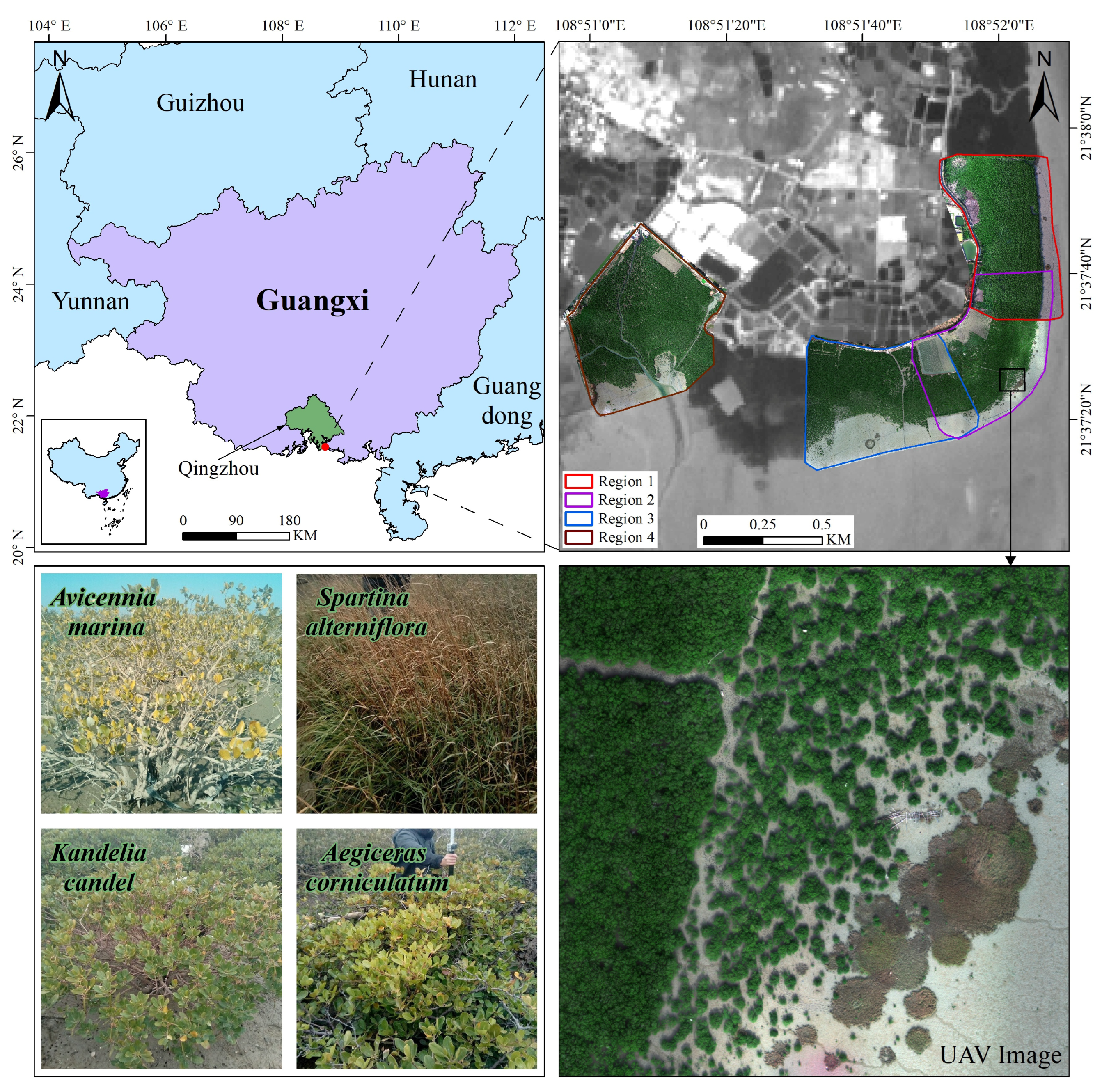
2.1. Study Area

Qinzhou City, Guangxi Province, China, is located on the southern coast of Guangxi and the northern shore of Beibu Gulf. It belongs to the subtropical–tropical transitional marine monsoon zone. The annual average temperature is above 22 °C, the average temperature of the coldest month is above 13 °C, and the annual precipitation is 1500–2000 mm, making it a suitable area for mangrove growth. Guangxi is rich in mangrove species [34], with a total area of 9330.34 hectares in 2019. The mangroves in Guangxi Province account for about 1/3 of the mangrove area in China. The mangroves in Qinzhou City account for about 1/3 of the total mangrove area in Guangxi. This paper’s study area is in the Beibu Gulf coastline region of Qinzhou City (21°37′10″N–21°38′15″N, 108°50′55″E–108°52′10″E), which has wetland woody plant communities composed of evergreen trees or shrubs with mangrove plants as the main component, including typical mangrove vegetation, such as Kandelia candel, Aegiceras corniculatum, and Avicennia marina. To protect the mangrove ecosystem from deterioration, the Chinese government has taken a series of measures, and in recent years, China has made positive progress in mangrove protection and restoration, with the total area of mangroves gradually increasing. Figure 1 shows the location of the study area. In this paper, the overall study area was divided into four blocks (Regions 1, 2, 3, and 4) for the experiments on the classification of mangrove communities.

2.2. Data Source

2.2.1. UAV Data Acquisition and Preprocessing

UAV multispectral images were acquired over two time periods: (1) From November 19 to 21, 2020, the DJI Phantom4 Multispectral (P4M) UAV was used for acquiring the images. The P4M is equipped with the FC6360 sensor, which integrates a visible light camera and five multispectral cameras (Blue, Green, Red, Red Edge, and NIR), responsible for visible light and multispectral imaging, respectively. The P4M flew at a height of 100 m, with a course overlap rate of 80% and a side overlap rate of 75%. The centimeter-level positioning system is integrated on the P4M, and the horizontal positioning accuracy is 0.1 m. (2) From 8 to 14 January 2021, the DJI MATRICE 210 (M210) UAV was used for acquiring the images. The M210 is equipped with Micasense’s RedEdge-MX sensor, which integrates five multispectral cameras (Blue, Green, Red, Red Edge, and NIR) to acquire multispectral images. The flight altitude of the M210 was 105 m, and the heading overlap rate and the side overlap rate were both 80%. M210 is equipped with a DLS2 positioning device, with a horizontal positioning accuracy of 2 m to 3 m. The flight time of both drones was from 10:00 to 15:00 (UTC + 08:00). The lens direction was vertically downward when the sensor was shooting, and the photos were taken at 3 s intervals. Each flight used the sensor to capture the correction plate provided by Micasense to obtain a new correction image, which provided a benchmark for radiometric calibration in subsequent image processing.

Table 1. Sensor parameters.

Sensors	Number of Bands	Spectral Bands	Sensor’s Resolution	Spatial Resolutions (cm)	Number of Images
FC6360	5	Blue (434–466 nm) Green (544–576 nm) Red (634–666 nm) Red edge (714–746 nm) NIR (814–866 nm)	1600 × 1300	5.84	59,658
RedEdge-MX	5	Blue (455–495 nm) Green (540–580 nm) Red (658–678 nm) Red edge (707–727 nm) NIR (800–880 nm)	1280 × 960	6.67	28,370

displays the remaining sensors’ parameters.

The obtained UAV images were processed by using Pix4D mapper software. Some of the main steps are importing the image, checking quality, matching the image, performing aerial triangulation, generating a point cloud, and finally generating a digital orthophoto model (DOM) and a digital surface model (DSM), with a spatial resolution of 0.07 m and a projected coordinate system of WGS 1984 UTM Zone 49N.

2.2.2. Field Investigation and Generation of a Semantic Label

To evaluate the classification accuracy of mangrove communities, field investigations were conducted from 21 to 24 November 2020; from 8 to 14 January 2021; and from 4 to 16 April 2021. We used Hi-Target V90 GNSS RTK (real-time kinematics) to record sample geographic coordinates (horizontal accuracy of 0.25 m + 1 ppm) and land-cover types and used the iHand30 handheld controller to take their pictures. We used P4M for transect shooting; the flight altitude was 30 m. Using the above two methods and auxiliary images, we identified land-cover types and made semantic label data through visual interpretation. The land-cover types in the study area are Avicennia marina, death mangroves, Kandelia candel, terrestrial vegetation, Aegiceras corniculatum, artifacts, mudflats, Spartina alterniflora, and water bodies. A total of 4060 sample datasets were obtained by combining the actual measurement and visual interpretation. The particular details are displayed in

Table 2. Summary of sample datasets.

Land-Cover Types	Abbreviations	Samples	Image Features	Interpretation Features
Avicennia marina	AM	850		Dark green, irregular shape, close to the sea
Death mangrove	DM	235		Dark purple and claybank, irregular shape
Kandelia candel	KC	525		Bottle green, a circle or ellipse, close to the shore
Terrestrial vegetation	TV	230		Green, no uniform shape, scattered on the shore
Aegiceras corniculatum	AC	205		Light green, relatively fine texture, closest to the shore
Artifact	AF	470		White and bright, square, scattered in mangroves
Mudflat	MF	730		Hoary and flesh-colored, mostly on the periphery of vegetation
Spartina alterniflora	SA	400		Taupe and black, most are circles, closest to the sea
Water Body	WB	415		Wathet blue, most are banded

.

2.3. Methods

In this paper, we developed an improved algorithm, MCCUNet, and compared it with DeepLabV3+ and HRNet to assess its efficacy in classifying a mangrove community. A UAV multidimensional dataset was constructed and combined with RFE–PCA dimension reduction and three CNN algorithms to explore the feasibility of combining a deep-learning algorithm with dimension reduction. Three transfer-learning strategies were proposed to explore the applicability and classification accuracy of different transfer-learning strategies. Figure 2 depicts the experimental procedure.

2.3.1. Construction and Dimension Reduction of Multidimensional Image Datasets

In this paper, we used UAV’s DOM to construct a multidimensional dataset. The steps are as follows: (1) ENVI 5.6 software was used to extract the TFs of the original 5 spectral bands, a total of 40 TFs in 8 categories (mean, variance, homogeneity, contrast, dissimilarity, entropy, angular second moment, and correlation). The movement window was 3 × 3, the co-occurrence shift was 1, and the grayscale quantization level was 64. (2) ENVI 5.6 software was used to calculate and extract a total of 45 vegetation indices (VIs) to enhance the spectral differences between different mangrove communities (Appendix A). Then TFs, VIs, DOM, and DSM were combined to generate multidimensional datasets. To investigate the impact of various image-feature combinations on the classification accuracy of mangrove communities, four feature datasets were constructed (

Table 3. Feature datasets containing different image-feature combinations and their number changes.

Scenarios	Feature Datasets	Descriptions	Number of Original Features	After High Correlation Elimination	After RFE→PCA	Number of Final Features
1	OS	DOM and DSM	6	-	-	6
2	OST	DOM, DSM, and TFs	46	24	14→9	9
3	OSV	DOM, DSM, and VIs	51	27	16→9	9
4	OSTV	DOM, DSM, TFs, and VIs	91	45	24→12	12

).

In this paper, recursive feature elimination (RFE) and principal component analysis (PCA) algorithms were combined to reduce the dimension of multidimensional datasets. The steps are as follows: (1) Using Rstudio software to remove highly correlated TFs and VIs, 18 low-correlation TFs and 21 low-correlation VIs were screened out. (2) Using the RFE algorithm, the variables were optimized for the TFs and the VIs after removing the high correlation, and 8 TFs and 10 VIs with high importance were selected. (3) Using ENVI 5.6 software, PCA dimension reduction was performed on the optimized TFs and VIs and the first three principal components with a contribution rate greater than 90% were selected. Table 3 displays the feature changes of different feature datasets.

2.3.2. Construction of Mangrove Community Classification Model Based on CNN Algorithms

• DeepLabV3+

As shown in Figure 3, the DeepLabV3+ method is divided into an encoder and a decoder. In the encoder, first Xception upgraded with Atrous convolution is used as the backbone network, and this decreases the number of parameters, while improving performance, and then Atrous spatial pyramid pooling (ASPP) is used, achieving an increased receptive field without reducing the training image resolution. In the decoder, to take into account the location information and semantic features, the low-level and high-level features are fused, refined, and then up-sampled to obtain the classification results.

• HRNet

Figure 4 illustrates the structure of the HRNet algorithm. The main body is divided into four stages. Each stage expands a branch relative to the previous one. The size of the feature output by this branch is reduced to 1/2, and the number of channels of the feature is expanded to 2 times. The algorithm has two main characteristics. One is to replace the traditional serial method with the parallel method of sub-networks with different resolutions to improve the accuracy of predicting the spatial information of the image; the other is to use repeated multiscale fusion to ensure exchange of information between different sub-networks at multiple resolutions, thus improving the accuracy of predicted images.

• MCCUNet

In this study, we modified the encoder and the decoder of the DeepLabV3+ algorithm. Figure 5 depicts the overall structure of the MCCUNet algorithm. The specific improvements are classified into two aspects.

(1)

As shown in Figure 6, we replaced the depth-wise convolution of size 3 × 3 for down-sampling in Xception, the backbone network of the encoder, with mixed depth-wise convolution (MixConv) [35], by adding convolution kernels of a larger size to increase the receptive field, thereby improving the performance. So that larger convolution kernels were added without increasing the number of parameters too much, the number of convolution kernels increased layer by layer, that is, from the first down-sampling layer containing two convolution kernels to the third down-sampling layer containing four convolution kernels, and the number of channels of convolution kernels of different sizes adopted an exponential partition (for example, if a down-sampling layer with four convolution kernels has a total of 64 channels, then the number of channels divided exponentially by each convolution kernel is (32, 16, 8, 8)). In addition, the convolutions in ASPP were replaced with depth-wise separable convolutions to reduce the number of parameters without affecting the accuracy.

(2)

To obtain edge detail features and further enhance the segmentation performance, more low-level features were added to the decoder (Figure 5) on the basis of the original encoder. After improvement, low-level features with sampling coefficients of 1/2, 1/4, and 1/8 were added. To not influence the expression of high-level semantic features, the number of channels of the three low-level features was reduced to 48 and then merged with the high-level semantic features. The features were then refined by two 3 × 3 depth-wise separable convolutions.

• Models for the classification of mangrove communities

In this paper, to classify mangrove communities, we constructed different models by using three deep-learning algorithms (DeepLabV3+, HRNet, and MCCUNet) with four feature datasets (OS, OST, OSV, and OSTV) in Regions 1 and 4 and calculated the overall classification accuracy. Then we quantitatively evaluated the differences in their performance in classifying mangroves to demonstrate the effectiveness of the MCCUNet algorithm. Simultaneously, we quantitatively evaluated the impact of different combinations of image features on classification performance through the difference in the average classification accuracy.

Table 4. Classification models for mangrove communities and the combination scenario of their image features.

Regions	Algorithms	Groups	Feature Datasets	Scenarios	Number of Images of Each Scenario
Region 1 + Region 4	DeepLabV3+	Group 1	OS	1	1 × 105
			OST	2
			OSV	3
			OSTV	4
	HRNet	Group 2	OS	1	1 × 105
			OST	2
			OSV	3
			OSTV	4
	MCCUNet	Group 3	OS	1	1 × 105
			OST	2
			OSV	3
			OSTV	4

depicts the specific scenarios.

On the basis of the models in Table 4, this paper conducted research from the following two aspects:

(1)

When the algorithm is identical but the feature dataset is different: Taking the MCCUNet algorithm as an example, we compared Scenarios 2 and 1 in Group 3 to explore the impact of adding TFs on the categorization of mangrove communities. We compared Scenarios 3 and 1 to explore the impact of adding VIs, and we compared Scenarios 4 and 1 to explore the impact of adding TFs and VIs.

(2)

When the feature dataset is identical but the algorithm is different: Taking the OSTV feature dataset as an example, we compared Scenario 4 of Groups 1~3 to explore the differences in the classification performance of DeepLabV3+, HRNet, and MCCUNet and then evaluated the effectiveness of the improved MCCUNet.

The training methods of all the models in Table 4 were identical; that is, the training data were randomly divided into datasets with a size of 256 × 256; data were enhanced (random rotation, horizontal or vertical flipping, and channel swapping); and 80% of the data were randomly selected as training data, while the remaining 20% were test data. The Adam method [36] was chosen to optimize the model, with an initial learning rate = 10⁻³, betas = (0.9, 0.999), and weight decay = 0. The focal loss was chosen as the model’s loss function to somewhat alleviate the category imbalance (parameter γ = 2), and the training epoch was set at 10.

2.3.3. Transfer Learning Strategies for Mangrove Communities

This paper proposed three transfer learning strategies, using the MCCUNet algorithm, based on model-based transfer learning and combined with different phase and sensor UAV images of different regions.

• Frozen Transfer Learning (F-TL)

We took Regions 1 and 4 as the source domain and Regions 2 and 3 as the target domain and transferred the weight parameters of the model in the source domain to the initial model in the target domain as its pretraining weights. Then we reduced the learning rate of the weight parameters of the backbone network of the model in the target domain to 0 and the others to 1/10 of the learning rate of the model in the source domain. Finally, we trained the model in the target domain multiple times and selected the model with the highest training accuracy for prediction. The specific process is shown in Figure 7.

• Fine-Tuned Transfer Learning (Ft-TL)

We took Regions 1 and 4 as the source domain, Regions 2 and 3 as the target domain, and the weight parameters of the source domain model as pretraining weights for the initial model in the target domain. When training the model in the target domain, we reduced the learning rate of the parameters of the backbone network of the model in the target domain to 1/100 of the model’s training in the source domain, and the learning rates of the remaining parameters were reduced to 1/10 of the model’s training rate in the source domain. Finally, the model with the highest training accuracy in the target domain was selected for prediction. The specific process is shown in Figure 8.

• Sensor-and-Phase Transfer Learning (SaP-TL)

We took Regions 1 and 4 from 8 to 14 January 2021, as the source domain and divided Regions 1 and 4 from 19 to 21 November 2020, into two target domains. The parameters in the source domain were transferred to the models of the two target domains. The learning rate of the model parameters in the two target domains was decreased to 1/10 of the learning rate in the source domain for training the model in the target domain, and the model with the highest training accuracy in the two target domains was selected for prediction. The specific process is shown in Figure 9.

Table 5. Transfer-learning classification schemes for mangrove communities.

Algorithms	Strategies	Groups	Source Domain	Target Domain	Feature Datasets	Scenarios	Number of Each Scenario
MCCUNet	“F-TL”	Group I	Region 1 + Region 4	Region 2 + Region 3	OS	1	1 × 105
					OST	2
					OSV	3
					OSTV	4
	“Ft-TL”	Group II	Region 1 + Region 4	Region 2 + Region 3	OS	1	1 × 105
					OST	2
					OSV	3
					OSTV	4
	“SaP-TL”	Group III	Region 1 + Region 4 (2021.01)	Region 1 (2020.11)	OS	1	1 × 105
					OST	2
					OSV	3
					OSTV	4
				Region 4 (2020.11)	OS	1	1 × 105
					OST	2
					OSV	3
					OSTV	4

presents the specific transfer learning classification schemes of mangrove communities according to the three transfer-learning strategies. To explore the applicability of different transfer-learning strategies to the classification of mangrove communities, in this study, we conducted research from the following four aspects: (1) Taking Group I as an example, we compared Scenarios 1 to 4 in Group I and measured the classification accuracy of mangrove communities when using different feature datasets to analyze the differences in their transfer-learning performance in identical areas and time phases. (2) We compared Scenarios 1 to 4 in Group I with Scenarios 1 to 4 in Group 3 in Table 4 to analyze the differences in the classification accuracy of the F-TL strategy when using identical feature datasets and then explored the feasibility of the transfer learning of frozen model parameters. (3) We compared Scenarios 1 to 4 of Group I and Group II to analyze the differences in the classification accuracy of the F-TL strategy and the Ft-TL strategy when using identical feature datasets and then explored the importance of fine-tuning model parameters for transfer learning. (4) We compared Scenarios 1 to 4 in Group III with Scenarios 1 to 4 in Group 3 in Table 4 to analyze the differences in the classification accuracy of the SaP-TL strategy when using identical feature datasets and then verified the transferability between different time phases and sensors images.

The pretraining weights used by the transfer-learning models in different scenarios were the weight parameters of the best training model obtained by the model corresponding to the scenario in the classification scheme. The optimizer of all models was Adam, with a learning rate = 10⁻³, betas = (0.9, 0.999), and weight decay = 0. The focal loss was chosen as the model’s loss function (parameter γ = 2). In the F-TL strategy, the learning rate of all the weight parameters, except for those of the backbone network, was 10⁻⁴. In the Ft-TL strategy, the learning rate of the weight parameters of the backbone network was 10⁻⁵, and that of the rest was 10⁻⁴. In SaP-TL, the learning rate of all the weight parameters was 10⁻⁴.

2.3.4. Accuracy Assessment

To evaluate the performance of different mangrove classification models, the confusion matrix and four precision indicators were used in this study, among which the precision indicators included overall classification accuracy (OA) [37], user accuracy (UA), producer accuracy (PA), and the F1–score. OA was used to quantitatively evaluate the differences in the accuracy of different classification models, and the F1–score and the confusion matrix were used to quantitatively analyze the differences among different models in accurately classifying various land-cover types. In addition, McNemar’s chi-square test [38] was used to evaluate the significance of the differences between the classification results of different models.

3. Results

3.1. Results Analysis of Mangrove-Community Classification with Different Feature Datasets

Table 6. Statistical difference between classification results of different feature datasets, using McNemar’s test.

Regions	Algorithms	OS vs. OST	OS vs. OSV	OS vs. OSTV	OST vs. OSTV	OSV vs. OSTV
Region 1	DeepLabV3+	17.29 *	14.52 *	34.13 *	65.69 *	65.64 *
	HRNet	5.49 *	2.89	21.60 *	6.21 *	9.39 *
	MCCUNet	2.56	7.26 *	20.10 *	10.32 *	7.04 *
Region 4	DeepLabV3+	1.39	0.00	0.06	0.45	0.00
	HRNet	8.31 *	2.37	4.67 *	0.84	0.14
	MCCUNet	6.72 *	7.26 *	8.65 *	0.50	0.00

* In the 95% confidence interval, the value x² > 3.84 shows that the differences are significant.

presents the significant differences between the classification results of different feature datasets, using an identical algorithm (i.e., the algorithm based on OA) to show the impact of high-dimensional datasets on the classification performance of mangrove communities after RFE–PCA dimension reduction is combined with different algorithms. Taking the MCCUNet algorithm as an example, we can see that the classification results using the OSV or OSTV feature dataset and those using the OS feature dataset differed significantly in both regions, and the chi-square value between the classification results using the OSTV feature dataset and those using the OS feature dataset is the largest in both regions (x² = 20.1 in Region 1, and x² = 8.65 in Region 4). These events demonstrate that the algorithm’s classification performance is somewhat impacted by the addition of features following dimension reduction, and the addition of a combination of multiple features has a greater impact than that of a single feature.

Figure 10 shows the growth rate of the F1–score of different mangrove communities (the growth rate is the difference in the F1–scores between the OST, OSV, and OSTV feature datasets and the OS feature dataset). In the three mangrove communities, the means of the growth rates of the F1–score of AM and KC were both greater than 3%, proving that, after the RFE–PCA dimension reduction of high-dimensional datasets, the combination with CNN algorithms had a certain positive effect on the classification performance of mangrove communities. Furthermore, all three mangrove communities had the highest mean of the growth rate of F1–score after the addition of both TFs and VIs (OSTV feature dataset), and the OSTV feature dataset combined with the MCCUNet algorithm allowed KC to achieve the highest growth rate of F1–score, i.e., 43.23%, in Region 4.

Figure 11 shows the species-distribution map when using the four feature datasets in Regions 1 and 4 based on the DeepLabV3+, HRNet, and MCCUNet algorithms, where there are some differences in the trends of different land-cover types.

When using the DeepLabV3+ algorithm, in Region 1, the classification results of the DM were decreased after adding TFs (OST) or Vis (OSV), and most of the DMs were misclassified as MF, while the classification results of the DM were substantially improved after adding both VIs and TFs (OSTV). In Region 4, the variation trend of the classification results of the AC was different from those of the DM, which improved after adding Vis.

When using the HRNet algorithm, in Region 1, the addition of either TFs (OST) or VIs (OSV) greatly improved the classification results of KC, while the simultaneous addition of TFs and Vis (OSTV) seemed to lead to a small overestimation of the distribution range of KC. In Region 4, the classification results of TV and KC achieved the best when adding TFs and Vis (OSTV).

When using the MCCUNet algorithm, in Region 1, the classification results of the WB decreased after the addition of TFs (OST), while the classification results of the WB improved after the addition of VIs (OSV). Moreover, the classification accuracy of the WB was further improved after the addition of TFs and Vis (OSTV). In Region 4, the trend of change in the classification results of KC was different from that of the WB, which improved after the addition of TFs (OST).

The above results proved that the addition of TFs and VIs improved the classification results of each land-cover type, in which most of the classification results of the three mangrove vegetations were best achieved by combing the TFs and Vis (OSTV).

3.2. Evaluation of Classification Performance Using the MCCUNet Algorithm

Figure 12 shows the difference in the overall classification accuracy (OA) between the MCCUNet algorithm and the DeepLabV3+ and HRNet algorithms when using four feature datasets that needs to be analyzed in two regions.

(1)

In Region 1, the three algorithms achieved satisfactory OA when using four feature datasets, and all the OA values were above 75%. The trend of change in the OA of the MCCUNet algorithm was more stable than that of the DeepLabV3+ and HRNet, and the MCCUNet algorithm achieved the highest OA (96.7%), which was 3.5% and 4.08% higher than those of the DeepLabV3+ and HRNet algorithms, respectively. Furthermore, when using the OSV feature dataset, the OA of the MCCUNet and DeepLabV3+ algorithms differed the most, reaching 13.59%, and there was a significant difference between the classification results of the MCCUNet and DeepLabV3+ algorithms within the 95% confidence interval (

Table 7. Statistical differences between the classification results of the three algorithms for feature datasets in different regions, using McNemar’s test.

Regions	Feature Datasets	MCCUNet vs. DeepLabV3+	MCCUNet vs. HRNet	DeepLabV3+ vs. HRNet
Region 1	OS	7.14 *	16.10 *	30.23 *
	OST	38.64 *	0.03	42.67 *
	OSV	43.56 *	0.02	45.38 *
	OSTV	0.19	26.68 *	21.60 *
Region 4	OS	2.21	2.57	9.09 *
	OST	5.94 *	2.53	0.64
	OSV	0.70	3.45	9.38 *
	OSTV	1.79	6.86 *	2.12

* In the 95% confidence interval, the value x² > 3.84 shows that the differences are significant.

). When using the OSTV feature dataset, the OA of the MCCUNet and HRNet algorithms differed by a maximum of 8.93%, and within the 95% confidence interval, the classification results of the MCCUNet and HRNet algorithms also differed significantly (Table 7).

(2)

In Region 4, the lowest OA among the three algorithms was 90%, and the trend of variation in the OA of the DeepLabV3+ and HRNet algorithms was more stable than that in Region 1. When employing the OSTV feature dataset, all three algorithms had the highest OA, among which the highest OA (97.24%) of the MCCUNet algorithm was 1.03% and 2.07% higher than that of the DeepLabV3+ and HRNet algorithms, respectively. Furthermore, according to McNemar’s chi-square test (Table 7), within the 95% confidence interval, there was a significant difference between the classification results of MCCUNet and HRNet algorithms when using the OSTV feature dataset, while the opposite was true between the MCCUNet and DeepLabV3+ algorithms.

Figure 13 shows the species-distribution map of three algorithms (DeepLabV3+, HRNet, and MCCUNet), using two feature datasets (OST and OSTV), that needs to be analyzed in two regions.

(1)

In Region 1 (Figure 13a,b), when using the OST feature dataset (Figure 13a), there was a large difference between the abilities of the three algorithms to identify the DM. Among them, the MCCUNet algorithm had the best ability to identify the DM, and the overall distribution and the boundary contour of the DM in its classification results were relatively complete, while the DeepLabV3+ algorithm misclassified most of the DM as part of the MF. This phenomenon corresponded to what the confusion matrix exhibited (Figure 14a). Furthermore, when comparing the classifications while using the MCCUNet algorithm, we can see that the edge and the middle part of the DM in the HRNet-algorithm-based classifications appeared to be confused with AF and TV. When using the OSTV dataset (Figure 13b), there were certain differences in the descriptions of KC between the classification results of the three algorithms. The MCCUNet algorithm outperformed the others in identifying KC, while the classification results of the DeepLabV3+ and HRNet algorithms showed confusion between AM and KC, and this was consistent with the phenomenon that KC was misclassified as AM in the confusion matrix (Figure 14b).

(2)

In Region 4 (Figure 13c,d), when using the OST feature dataset (Figure 13c), the three algorithms also showed large differences in the ability to identify the DM. The distribution range of the DM was the most complete in the classification result of the MCCUNet algorithm, while both DeepLabV3+ and HRNet algorithms misclassified the DM as TV and part of the MF. Furthermore, DeepLabV3+ and HRNet misclassified AC as KC to different degrees, while in the classification result of MCCUNet, this situation was greatly improved, and this is consistent with the description of the corresponding confusion matrix (Figure 14c). When using the OSTV feature dataset (Figure 13d), there were differences in the distribution range of AC in the classification results of the three algorithms. Among them, the MCCUNet had the best ability to identify AC, and only a small number of instances of AC and KC were confused, while in the classification results of DeepLabV3+ and HRNet, the degree of confusion between AC and KC was more serious, and this phenomenon was also reflected in the corresponding confusion matrix (Figure 14d).

3.3. Evaluation of the Effect of Different Transfer-Learning Strategies on Mapping Mangrove Communities

3.3.1. Classification Results of Mangrove Communities Based on the Frozen-Transfer-Learning Strategy

This study compared the differences in the F1–scores of each land-cover type by using the four feature datasets under the F-TL strategy in two regions (Regions 2 and 3), using the MCCUNet algorithm to evaluate quantitatively the applicability of the F-TL strategy to the classification of mangrove communities.

(1)

In Region 2 (Figure 15), the classification accuracy of AM and KC was good; that is, both had an F1–score above 80% and both had the highest F1–score when using the OS dataset (F1–scores were 92.73% and 94.16%, respectively). Except for the mangrove communities, the F1–scores of the MF and SA fluctuated widely, with a difference of 26.55% and 44.53% between the highest and lowest F1–scores of the two, respectively.

(2)

Compared to Region 2, in Region 3 (Figure 15), the classification accuracy of both AM and KC improved (F1–scores of both were higher than 90%), with AM achieving the highest accuracy, i.e., 93.8%, using the OSV feature dataset, and KC achieving the highest accuracy, i.e., 99.5%, using the OST feature dataset. Except for mangrove communities, the range of variation in F1–scores of the MF was more stable in Region 3, with the D-value between the highest and lowest F1–scores being 4.65%, while the F1–scores of SA varied greatly, with the highest F1–score at 59.38% and the lowest F1–score at 15.09%.

To evaluate qualitatively the impact of the F-TL strategy on the classification of mangrove communities, based on the MCCUNet algorithm, the effects of classifying different land-cover types by using the four feature datasets after the implementation of transfer learning were compared in two regions.

(1)

In Region 2 (Figure 16a,b), the classification results of the four feature datasets showed large differences in the descriptions of AM and KC (Figure 16a). The OST feature dataset was not satisfactory, misclassifying KC in most cases as AM. In the classification results using the other three feature datasets, this phenomenon improved. However, compared with the OSV feature dataset, the OS and OSTV feature datasets misclassified some of the AM as KC. The four feature datasets also showed differences in describing SA (Figure 16b). When using the OSV feature dataset, most of the SA was misclassified as part of the MF, and this phenomenon was improved to a certain extent when using the OSV feature dataset, while the overall outline of the SA was still incomplete. When using the OS dataset, the SA edge was relatively complete, while a small part of its interior was still misclassified as part of the MF, and when using the OST dataset, the problem of the missing inside and edge of the SA was almost resolved.

(2)

In Region 3 (Figure 16c,d), there was a certain difference between the classification results of the four feature datasets in describing the WB and SA. As shown in Figure 16c, the classification result from using the OST feature dataset was disappointing, and most of the WB was misclassified as part of the MF, while the single WB in the lower left corner was relatively complete. In the classification result using the OS feature dataset, the tributary could not be identified, while in that using the OSV and OSTV feature datasets, the WB was well identified. Moreover, the WB seemed to be overestimated when using OSTV the feature dataset. It is evident from Figure 16d that most of the SA was misclassified as part of the MF in all classification results. Except for the OSV feature dataset, some of the SA was misclassified as AM when using other feature datasets. Similarly, SA was misclassified as KC when using all other feature datasets, except for the OST feature dataset.

In this study, we quantitatively analyzed the confusion matrix and the change in F1–score before (Region 1) and after (Region 2) transfer learning to investigate the impact of the F-TL strategy on the classification of different land-cover types. As seen in Figure 17b, the F1–score of AM showed a downward trend, and its F1–score decreased by 0.60~11.21%, due to the increased confusion between KC and AM after the implementation of transfer learning (Figure 17a). When using the OS feature dataset, the F1–score of KC increased by 2.09% (Figure 17b), while when using the remaining feature datasets, its F1–score reduced by 4.76~9.54%, because some part of the KC was misclassified as AM and part of the MF after the implementation of transfer learning (Figure 17a). Except for mangrove communities, the F1–scores of the MF and SA showed a downward trend and the F1–score dropped significantly when using the OSV and OSTV datasets, in which the F1–scores of the MF dropped by 34.97% and 24.82%, respectively, while the F1–scores of SA dropped, respectively, by 43.69% and 18.46%. The reason was that a small part of the WB and most of the SA were misclassified as part of the MF (Figure 17a).

3.3.2. Classification Results of Mangrove Communities Based on the Fine-Tuned Transfer Learning Strategy

This study compared the differences in the F1–scores of each land-cover type, using the four feature datasets under the Ft-TL strategy in two regions (Regions 2 and 3), using the MCCUNet algorithm to evaluate quantitatively the applicability of the Ft-TL strategy in the classification of mangrove communities.

(1)

In Region 2 (Figure 18), both mangrove communities (AM and KC) showed good F1–scores, with an F1–score of more than 84%. AM achieved the highest F1–score (93.04%) when the OSV feature dataset was used, while KC achieved the highest F1–score (94.69%) when the OS feature dataset was used. Except for the mangrove communities, the F1–scores of the MF and SA fluctuated a lot, and the MF achieved the highest and lowest F1–scores when the OS and OSTV feature datasets were used, with a difference of 22.25%, while SA achieved the highest and lowest F1–scores when the OST and OSTV feature datasets were used, with a difference of 29.61%.

(2)

In Region 3 (Figure 18), the F1–score of mangrove communities (AM and KC) was above 90%, higher than that in Region 2, and KC and AM achieved the highest F1–scores, of 98.02% and 92.87%, using the OS and OST feature datasets, respectively. Except for the mangrove communities, the trend of change in the F1–scores of the MF was more stable in Region 3 than in Region 2, and the D-value between the highest and lowest F1–scores was 6.55%. The F1–score of SA showed a larger variation, and its highest F1–score was 68.42% (using the OS feature dataset) and lowest F1–score was 40% (using the OSTV feature dataset).

To qualitatively evaluate the impact of the Ft-TL strategy on the classification effect of mangrove communities, in Regions 2 and 3, based on the MCCUNet algorithm, the effects of classifying different land-cover types using the four feature datasets after transfer-learning implementation were compared.

(1)

In Region 2 (Figure 19a,b), after transfer-learning implementation, the classification results of the four feature datasets showed a large difference in the descriptions of the distribution ranges of AM and KC (Figure 19a). The description of the distribution range of AM and KC had a large deviation when using the OST feature dataset, where some KC was misclassified as AM, and the situation was improved to varying degrees when using the remaining feature datasets. However, the classification results of OS and OSTV feature datasets overestimated KC. In comparison, the OSV feature dataset was more accurate in describing the distribution of AM and KC. Furthermore, the classification results of the four feature datasets differed significantly in describing the distribution range of SA (Figure 19b); all four feature datasets misclassified SA as part of the MF. The accuracy with which the four feature datasets described SA is ranked from high to low as follows: OST > OS > OSV > OSTV. A small part of SA was misclassified as AM in the classification results of the OST feature dataset.

(2)

In Region 3 (Figure 19c,d), there were large differences in the classification results of the four feature datasets in describing the WB and SA. As shown in Figure 19c, part of the WB was misclassified as part of the MF when using the OST feature dataset. However, this phenomenon was improved in the classification results of the remaining feature datasets, while the WB was overestimated when using the OSTV feature dataset. The description of the WB was similar when using OS and OST feature datasets, while there was a hole in the middle of the WB when using the OS feature dataset; that is, a small part of the WB was misclassified as part of the MF, and this phenomenon was improved when using the OSV feature dataset. As shown in Figure 19d, most of the SA was misclassified as part of the MF, using the four feature datasets. Among them, the OS feature dataset was the best in classifying SA, followed by the OSV feature dataset, while the OSTV feature dataset was unsatisfactory in classifying SA.

To investigate the impact of the Ft-TL strategy on the classification of different land-cover types, we quantitatively analyzed the confusion matrix and the change in F1–score before (Region 1) and after (Region 3) transfer learning. Figure 20b shows that the F1–score of both mangrove communities tended to decrease, except using the OS feature dataset, with a range of 2.08~7.88%; while the F1–score of KC improved when using the OS feature dataset, the reason was that the degree of confusion between AM and KC weakened after transfer learning (Figure 20a). Except for mangrove communities, the F1–scores of MF, SA, and WB showed a downtrend when using the OSV and OSTV feature datasets, where the F1–score of the three showed decreasing ranges of 26.10~30.91%, 24.13~28.15%, and 4.86~10.43%, respectively. Moreover, the F1–score of WB showed an increasing trend when using the OS and OST feature datasets, with an increase of 8.24% and 7.63%, respectively, which was attributed to the fact that the phenomenon of MF being misclassified as WB was weakened after transfer learning (Figure 20a).

3.3.3. Classification Results of Mangrove Communities Based on the Sensor-and-Phase Transfer-Learning Strategy

To explore the transferability between images of different phases and sensors, this study selected Regions 1 and 4 based on the MCCUNet algorithm and four feature datasets, counted the average classification accuracy (F1–score) of each land-cover type under different feature datasets, and quantitatively evaluated the feasibility of SaP-TL.

(1)

In Region 1 (Figure 21), the F1–score of three mangrove communities, namely AM, KC, and AC, was above 85%, and the three mangrove communities all achieved the highest F1–score when using the OS feature dataset. Among them, the F1–score of AC had the smallest variation (the D-value between the highest and lowest F1–scores was 2.44%) and the F1–score of KC had the largest variation (the D-value between the highest and lowest F1–scores was 10.07%). Except for the mangrove communities, the trends of change in the F1–scores of the MF and the WB had a certain similarity; that is, the lowest F1–score was achieved when using the OST feature dataset and the highest F1–score was achieved when using the OSTV feature dataset, and the D-values between the highest and lowest F1–scores of the MF and the WB was 14.51% and 30.88%, respectively.

(2)

In Region 4 (Figure 21), among the three mangrove communities, the F1–scores of AM and AC was above 70%, while KC achieved the lowest F1–score, i.e., 16.67%, when the OST feature dataset was used. In addition, compared with Region 1, the F1–scores of AM and AC fluctuated more, with the D-values between the highest and lowest F1–scores being 23.03% and 15.42%, respectively. Except for the mangrove communities, the trend of change in the F1–scores of the MF and the WB was consistent when using the four feature datasets; that is, the MF and the WB obtained the highest and lowest F1–scores when using the identical dataset (lowest when using the OST feature dataset and highest when using the OSV feature dataset), and the D-values between the highest and lowest F1–scores of the two was 5.69% and 6.17%, respectively.

To analyze qualitatively the impact of the SaP-TL strategy on the classification effect of mangrove communities, this study selected Regions 1 and 4, based on the MCCUNet algorithm and four feature datasets, and the classification effects of different feature datasets after the implementation of transfer learning were compared.

(1)

In Region 1 (Figure 22a,b), the classification results from using the four feature datasets were significantly different in describing the distribution range of KC (Figure 22a). In all classification results, KC was misclassified as AM, and the KC classification accuracy of each feature dataset ranked from low to high as follows: OS > OSV > OSTV > OST. Except for the OSV feature dataset, the others had misclassified KC as AC. There were also great differences in the ability of the four feature datasets in recognizing the WB (Figure 22b). Among them, the OSTV feature dataset was the best in classifying the WB, and its edge contour was relatively clear, with almost no missing edge, while most of the WB in the classification results using the remaining feature datasets was misclassified as being part of the MF, and the contour of the WB was missing to a greater extent.

(2)

In Region 4 (Figure 22c,d), the classification results of the four feature datasets had large differences in describing the distribution range of KC and AM (Figure 22c). The OST feature dataset misclassified most of the KC as AM, but when using the remaining feature datasets, the situation was greatly improved, while when using the OS and OSTV feature datasets, there was some confusion in KC and AC. In contrast, the OSV feature dataset was the most accurate in describing KC. The four feature datasets provided different descriptions of the AC distribution range (Figure 22d). When using the OS and OST feature datasets, some AC was misclassified as AM, and this situation was improved to a certain extent when using the other two feature datasets, while when using the OSTV feature dataset, some AM was misclassified as KC. In contrast, when using the OSV feature dataset, the description of the distribution range of KC was more accurate.

To quantitatively evaluate the impact of the SaP-TL strategy on the classification accuracy of each land-cover type, this study selected Region 4 and analyzed the changes in the confusion matrix and the F1–score of each land-cover type before and after the implementation of transfer learning. The F1–scores of the three mangrove communities showed an upward trend when using the OS, OSV, and OSTV feature datasets (Figure 23b). Among them, the F1–score of AM increased by 1.84~3.09%, the F1–score of KC increased by 5.97~35.83%, and the F1–score of AC increased by 6.99~19.85%. The confusion matrix clearly indicated that the misclassification of KC and AC as AM was reduced after transfer-learning implementation (Figure 23a). When using the OST feature dataset, among the three mangrove communities, only the F1–score of AC improved by 3.21%, while the F1–scores of AM and KC decreased by 17.78% and 69.54%, respectively. The reason was that, after the implementation of transfer learning, the misclassification of AC as KC was reduced, while there was still some misclassification between KC and AC when using the OS and OSTV feature datasets. Meanwhile, KC was mostly misclassified as AM (Figure 23a). Except for the mangrove communities, the trend of variation in the F1–score of the MF and the WB had a certain consistency; that is, the F1–scores of both showed a downward trend when using the OS, OST, and OSTV feature datasets; both had the largest drop when using the OST feature dataset; and the F1–score of MF and WB decreased by 3.66% and 6%, respectively, due to an increase in the misclassification of the WB as part of the MF after the implementation of transfer learning (Figure 23a). Considering that the distribution range of mangroves between different time-phase images had not changed greatly, two land-cover types with relatively large changes, SA and the WB, were selected, and the classification results of the two before and after the SaP-TL strategy were compared (Figure 24).

3.3.4. Statistical Analysis of the Classification Accuracy of Mangrove Communities for Three Transfer-Learning Strategies

Figure 25 shows the statistical analysis of the average classification accuracy (F1–score) of each land-cover type under the F-TL strategy and the Ft-TL strategy. Compared with the F-TL strategy, in the Ft-TL strategy, the F1–score of each land-cover type clearly improved. For two mangrove communities, AM and KC, the mean of F1–score under the Ft-TL strategy was higher than that under the F-TL strategy, where the mean of F1–scores of AM and KC were improved by 0.47% and 2.25%, respectively. Except for the mangrove communities, the mean of F1–scores of the other three land-cover types under the Ft-TL strategy were also higher than those under the F-TL strategy. Among them, the means of the F1–scores of the MF, SA, and WB were improved by 3.05%, 10.88%, and 3.41%, respectively.

Figure 26 shows the statistical analysis of the F1–scores of each land-cover type before and after the implementation of the SaP-TL strategy. The F1–scores of mangrove communities improved by varying degrees after the implementation of transfer learning. Among them, the means of the F1–scores of KC and AC were improved by 4.60% and 5.69%, respectively. Except for the mangrove communities, there were differences in the trends of change in the F1–scores of different land-cover types after the implementation of transfer learning. Among them, under the SaP-TL strategy, the F1–score of SA increased by 0.58% and the fluctuation degree of the F1–score of SA decreased. Moreover, the means of the F1–scores of the MF and the WB decreased by 4.94% and 6.77%, respectively, under the SaP-TL strategy, and the fluctuation degree of the F1–score of the MF and the WB increased.

4. Discussion

This paper found significant differences in the overall classification accuracy (OA) of mangroves by deep-learning algorithms when using different image feature datasets (Figure 11). The OA of the MCCUNet algorithm when using the OST, OSV, and OSTV feature datasets was higher than the OA when using the OS feature datasets (DOM and DSM). In Region 4, the OA levels when using the OST, OSV, and OSTV feature datasets were improved by 4.66%, 6.38%, and 7.24%, respectively, compared with the OS feature datasets. There were significant differences between the classification results of different feature datasets (Table 6), and the classification accuracy was improved by combining the CNN algorithm with RFE–PCA dimension reduction of a high-dimensional dataset. This conclusion was consistent with that of Zhang et al. [39] and Liu et al. [40]. Zhang et al. (2021) [39] combined wavelet fusion and PCA dimension reduction, which improved the classification accuracy of wheat and vegetation by 0.59% and 1.58%, respectively. Liu et al. (2017) [40] introduced F-norm and PCA dimension reduction, which improved the overall accuracy of the CNN algorithm by 4.12%. In conclusion, combining dimension reduction with a deep-learning algorithm allows us to improve the classification accuracy of the model, which is also applicable to the classification of mangrove communities. Furthermore, according to the average classification accuracy (F1–score) of different mangrove communities when adding different image features (Figure 10), the addition of more feature information could improve the F1–score of mangrove communities. For KC, compared with adding the TFs alone, the F1–score after adding the TFs and the VIs was higher, and the mean of the F1–score was improved by 9.74%, which further proved that combining different feature information helps improve the classification accuracy of mangrove communities [41], thereby improving the classification performance of the model for mangrove communities.

Some studies have explored the ability of the DeepLabV3+ algorithm to identify vegetation [42,43], and the DeepLabV3+ algorithm had problems of unclear boundary segmentation and small area misjudgment [44]. This paper proposed an improved algorithm, MCCUNet, by replacing part of the convolution layers of Xception in DeepLabV3+ with mix depth-wise separable convolutions and adding two additional layers of low-level features to the decoder. According to the changes in the OA of different algorithms when using different feature datasets (Figure 12), compared with the DeepLabV3+ algorithm, the OA of the MCCUNet was higher except when the OS feature dataset was used in Region 4, where the OA improvement range was 1.03~13.59%, while McNemar’s chi-square test showed that the difference between the classification results of the MCCUNet algorithm and the DeepLabV3+ algorithm in Region 4 was not significant when using the OS feature dataset within the 95% confidence interval (Table 7), so the improvement in the algorithm was effective and the classification performance of the algorithm for mangrove communities was successfully improved. Furthermore, from the visual classification effect (Figure 13), the MCCUNet algorithm was better than the DeepLabV3+ algorithm in identifying the edge contour and distribution range of the features, which demonstrated the improved segmentation performance of the algorithm after modification. This study demonstrates that the MCCUNet algorithm has the ability to identify mangrove species with higher accuracy and clarify the spatial distribution of mangrove communities, thus providing a scientific basis for the conservation, ecological restoration, and sustainable development of mangrove ecosystems. In addition, the OA of MCCUNet was lower than that of the HRNet algorithm only when the OS feature dataset was used, while McNemar’s chi-square test showed that there was a significant difference between the classification results of the two when using the OS feature dataset in Region 1 within the 95% confidence interval (Table 7). So, there is more room for improving the algorithm. In future research, the classification performance of the algorithm may be further improved by adding further attention mechanisms to the network [45,46] or by replacing the basic structural units of the backbone network [47] to better apply to the identification of mangrove communities.

Among the three transfer-learning strategies proposed in this paper, since the research areas of the F-TL and Ft-TL strategies were both Regions 2 and 3, observing the difference in the F1–scores of land-cover type under two strategies, Ft-TL and F-TL (Figure 25), showed that the mean of the F1–scores of the five land-cover types under the Ft-TL strategy had improved compared with that of the F-TL strategy. The F1–scores of AM, KC, the MF, SA, and the WB increased by 0.47%, 2.25%, 3.05%, 10.08%, and 3.41%, respectively. This proved the importance of fine-tuning model parameters; that is, having more parameters for learning led to the better classification performance of the model, which is similar to the experimental results of Espejo-Garcia et al. [48]. However, the degree of fluctuation of the F1–scores of SA and the WB under the Ft-TL strategy was lower than that of the F-TL strategy (Figure 25); that is, the fine-tuned model was more stable, and this differed from the results of Espejo-Garcia et al. because of the difference in the pretraining dataset used. They used ImageNet for the pretraining dataset, which was quite different from the weeds they were studying, while this paper used images from Regions 1 and 4, which shared species with Region 2 and 3. In addition, our target domain was more similar to the source domain. For the SaP-TL strategy, in Regions 1 and 4, the means of the F1–scores of KC and AC improved after the implementation of transfer learning (Figure 26), and the average classification accuracy of KC and AC increased by 4.60% and 5.69%, respectively. This proved that the transfer learning of mangrove-community classification from UAV images of different phases and sensors was feasible, which was similar to the experimental results of Maung and Sasaki [49], though the study by Maung and Sasaki was not on the community scale and only distinguished mangroves from non-mangroves. Furthermore, the F1–score of the WB before and after the implementation of the SaP-TL strategy was quite different, partly due to the imbalance of the training dataset [50]; that is, the distribution range of the WB in Region 1 was small, which made the proportion of the WB in the randomly cropped training dataset relatively small. Another main reason was that there were certain differences in the probability distribution between the UAV images of different phases and sensors. The above two eventually led to the model showing a certain degree of overfitting to the WB. This study demonstrated that the transfer-learning classification of mangrove communities is feasible in different regions and using time phases and sensors, and each mangrove species produced good classification accuracy. This method could extend and apply to other regions for mangrove species’ identification, monitoring of mangrove coverages and its structure species composition, and detection of invasive species. In future research, transfer learning may not be limited to the transfer of model parameters but may also start from data, through instance-based [51] or feature-based [52] transfer learning, to improve the similarity between the source and target domains and reduce the probability distribution difference between the source and target domains. Finally, the three methods allowed for an organic combination to achieve the best transfer-learning ability. At present, scholars have made achievements in similar directions [53].

5. Conclusions

In this study, mangrove communities were classified by using a new MCCUNet algorithm with UAV multispectral images. The applicability of three transfer-learning strategies in classifying mangrove communities and the differences in their classification were demonstrated. The MCCUNet algorithm presented in this study produced the best classification performance for mangrove communities with three deep-learning algorithms and achieved 97.24% overall classification accuracy (OA). The RFE–PCA dimension reduction improved the classification performance of deep-learning algorithms, with the OA increasing by 4.66~7.24%. The fine-tuned transfer-learning strategy achieved better classification accuracy than the frozen-transfer-learning strategy, and the F1–score of Spartina alterniflora increased by 4.77~19.56%. The sensor-and-phase transfer-learning strategy produced better transfer-learning classifications of mangrove communities across different phase and sensor images. All three transfer-learning strategies achieved high-accuracy classifications for mangrove communities, and the mean of the F1–score for mangrove communities was between 84.37% and 95.25%.

References

1. Maurya, K.; Mahajan, S.; Chaube, N. Remote sensing techniques: Mapping and monitoring of mangrove ecosystem—A review. Complex Intell. Syst. 2021, 7, 2797–2818. [Google Scholar] [CrossRef]
2. Donato, D.C.; Kauffman, J.B.; Murdiyarso, D.; Kurnianto, S.; Stidham, M.; Kanninen, M. Mangroves among the most carbon-rich forests in the tropics. Nat. Geosci. 2011, 4, 293–297. [Google Scholar] [CrossRef]
3. Fu, B.; He, X.; Yao, H.; Liang, Y.; Deng, T.; He, H.; Fan, D.; Lan, G.; He, W. Comparison of RFE-DL and stacking ensemble learning algorithms for classifying mangrove species on UAV multispectral images. Int. J. Appl. Earth Obs. Geoinf. 2022, 112, 102890. [Google Scholar] [CrossRef]
4. Wang, L.; Jia, M.; Yin, D.; Tian, J. A review of remote sensing for mangrove forests: 1956–2018. Remote Sens. Environ. 2019, 231, 111223. [Google Scholar] [CrossRef]
5. Li, Q.; Wong, F.K.K.; Fung, T. Classification of Mangrove Species Using Combined WordView-3 and LiDAR Data in Mai Po Nature Reserve, Hong Kong. Remote Sens. 2019, 11, 2114. [Google Scholar] [CrossRef] [Green Version]
6. Yan, Y.; Deng, L.; Liu, X.; Zhu, L. Application of UAV-Based Multi-angle Hyperspectral Remote Sensing in Fine Vegetation Classification. Remote Sens. 2019, 11, 2753. [Google Scholar] [CrossRef] [Green Version]
7. Diez, Y.; Kentsch, S.; Fukuda, M.; Caceres, M.; Moritake, K.; Cabezas, M. Deep Learning in Forestry Using UAV-Acquired RGB Data: A Practical Review. Remote Sens. 2021, 13, 2837. [Google Scholar] [CrossRef]
8. Ahmed, O.S.; Shemrock, A.; Chabot, D.; Dillon, C.; Williams, G.; Wasson, R.; Franklin, S.E. Hierarchical land cover and vegetation classification using multispectral data acquired from an unmanned aerial vehicle. Int. J. Remote Sens. 2017, 38, 2037–2052. [Google Scholar] [CrossRef]
9. Villoslada, M.; Bergamo, T.; Ward, R.; Burnside, N.; Joyce, C.; Bunce, R.; Sepp, K. Fine scale plant community assessment in coastal meadows using UAV based multispectral data. Ecol. Indic. 2020, 111, 105979. [Google Scholar] [CrossRef]
10. Manna, S.; Raychaudhuri, B. Mapping distribution of Sundarban mangroves using Sentinel-2 data and new spectral metric for detecting their health condition. Geocarto Int. 2018, 35, 434–452. [Google Scholar] [CrossRef]
11. Cao, J.; Leng, W.; Liu, K.; Liu, L.; He, Z.; Zhu, Y. Object-Based Mangrove Species Classification Using Unmanned Aerial Vehicle Hyperspectral Images and Digital Surface Models. Remote Sens. 2018, 10, 89. [Google Scholar] [CrossRef] [Green Version]
12. Jiang, Y.; Zhang, L.; Yan, M.; Qi, J.; Fu, T.; Fan, S.; Chen, B. High-Resolution Mangrove Forests Classification with Machine Learning Using Worldview and UAV Hyperspectral Data. Remote Sens. 2021, 13, 1529. [Google Scholar] [CrossRef]
13. Mahdianpari, M.; Salehi, B.; Rezaee, M.; Mohammadimanesh, F.; Zhang, Y. Very Deep Convolutional Neural Networks for Complex Land Cover Mapping Using Multispectral Remote Sensing Imagery. Remote Sens. 2018, 10, 1119. [Google Scholar] [CrossRef] [Green Version]
14. Hasan, M.; Ullah, S.; Khan, M.J.; Khurshid, K. Comparative analysis of svm, ann and cnn for classifying vegetation species using hyperspectral thermal infrared data. ISPRS—Int. Arch. Photogramm. Remote Sens. Spat. Inf. Sci. 2019, XLII-2/W13, 1861–1868. [Google Scholar] [CrossRef] [Green Version]
15. Wei, W.; Gu, H.; Deng, W.; Xiao, Z.; Ren, X. ABL-TC: A lightweight design for network traffic classification empowered by deep learning. Neurocomputing 2022, 489, 333–344. [Google Scholar] [CrossRef]
16. Lou, P.; Fu, B.; He, H.; Li, Y.; Tang, T.; Lin, X.; Fan, D.; Gao, E. An Optimized Object-Based Random Forest Algorithm for Marsh Vegetation Mapping Using High-Spatial-Resolution GF-1 and ZY-3 Data. Remote Sens. 2020, 12, 1270. [Google Scholar] [CrossRef] [Green Version]
17. Zhou, R.; Yang, C.; Li, E.; Cai, X.; Yang, J.; Xia, Y. Object-Based Wetland Vegetation Classification Using Multi-Feature Selection of Unoccupied Aerial Vehicle RGB Imagery. Remote Sens. 2021, 13, 4910. [Google Scholar] [CrossRef]
18. Chen, L.-C.; Zhu, Y.; Papandreou, G.; Schroff, F.; Adam, H. Encoder-Decoder with Atrous Separable Convolution for Semantic Image Segmentation. In Computer Vision—ECCV 2018; Springer International Publishing: Cham, Switzerland, 2018; pp. 833–851. [Google Scholar]
19. Sun, K.; Xiao, B.; Liu, D.; Wang, J. Deep High-Resolution Representation Learning for Human Pose Estimation. In Proceedings of the 2019 IEEE/CVF Conference on Computer Vision and Pattern Recognition (CVPR), Long Beach, CA, USA, 15–20 June 2019. [Google Scholar]
20. Xu, Z.; Zhou, Y.; Wang, S.; Wang, L.; Li, F.; Wang, S.; Wang, Z. A Novel Intelligent Classification Method for Urban Green Space Based on High-Resolution Remote Sensing Images. Remote Sens. 2020, 12, 3845. [Google Scholar] [CrossRef]
21. Ayhan, B.; Kwan, C. Tree, Shrub, and Grass Classification Using Only RGB Images. Remote Sens. 2020, 12, 1333. [Google Scholar] [CrossRef] [Green Version]
22. Liu, G.; Chai, Z. Image semantic segmentation based on improved DeepLabv3+ network and superpixel edge optimization. J. Electron. Imaging 2022, 31, 013011. [Google Scholar] [CrossRef]
23. LeCun, Y.; Bengio, Y.; Hinton, G. Deep learning. Nature 2015, 521, 436–444. [Google Scholar] [CrossRef] [PubMed]
24. Adhitya, Y.; Prakosa, S.W.; Köppen, M.; Leu, J.-S. Convolutional Neural Network Application in Smart Farming. In Communications in Computer and Information Science; Springer: Singapore, 2019; pp. 287–297. [Google Scholar]
25. Adhiwibawa, M.A.S.; Ariyanto, M.R.; Struck, A.; Prilianti, K.R.; Brotosudarmo, T.H.P. Convolutional neural network in image analysis for determination of mangrove species. In Proceedings of the Third International Seminar on Photonics, Optics, and Its Applications (ISPhOA 2018), Surabaya, Indonesia, 1–2 August 2018. [Google Scholar] [CrossRef]
26. Ahlswede, S.; Asam, S.; Röder, A. Hedgerow object detection in very high-resolution satellite images using convolutional neural networks. J. Appl. Remote Sens. 2021, 15. [Google Scholar] [CrossRef]
27. Memon, N.; Parikh, H.; Patel, S.B.; Patel, D.; Patel, V.D. Automatic land cover classification of multi-resolution dualpol data using convolutional neural network (CNN). Remote Sens. Appl. Soc. Environ. 2021, 22, 100491. [Google Scholar] [CrossRef]
28. Li, X.; Zhang, L.; Du, B.; Zhang, L.; Shi, Q. Iterative Reweighting Heterogeneous Transfer Learning Framework for Supervised Remote Sensing Image Classification. IEEE J. Sel. Top. Appl. Earth Obs. Remote Sens. 2017, 10, 2022–2035. [Google Scholar] [CrossRef]
29. Hussain, M.; Bird, J.J.; Faria, D.R. A Study on CNN Transfer Learning for Image Classification. In Advances in Intelligent Systems and Computing; Springer: Cham, Switzerland, 2018; pp. 191–202. [Google Scholar]
30. Weiss, K.; Khoshgoftaar, T.M.; Wang, D.D. A survey of transfer learning. J. Big Data 2016, 3, 1345–1459. [Google Scholar] [CrossRef] [Green Version]
31. Bhuiyan, A.E.; Witharana, C.; Liljedahl, A. Use of Very High Spatial Resolution Commercial Satellite Imagery and Deep Learning to Automatically Map Ice-Wedge Polygons across Tundra Vegetation Types. J. Imaging 2020, 6, 137. [Google Scholar] [CrossRef]
32. Zhang, D.; Ding, Y.; Chen, P.; Zhang, X.; Pan, Z.; Liang, D. Automatic extraction of wheat lodging area based on transfer learning method and deeplabv3+ network. Comput. Electron. Agric. 2020, 179, 105845. [Google Scholar] [CrossRef]
33. Liu, M.; Fu, B.; Fan, D.; Zuo, P.; Xie, S.; He, H.; Liu, L.; Huang, L.; Gao, E.; Zhao, M. Study on transfer learning ability for classifying marsh vegetation with multi-sensor images using DeepLabV3+ and HRNet deep learning algorithms. Int. J. Appl. Earth Obs. Geoinf. 2021, 103, 102531. [Google Scholar] [CrossRef]
34. Wang, H.; Yao, Y.; Dai, X.; Chen, Z.; Wu, J.; Qiu, G.; Feng, T. How do ecological protection policies affect the restriction of coastal development rights? Analysis of choice preference based on choice experiment. Mar. Policy 2022, 136, 104905. [Google Scholar] [CrossRef]
35. Tan, M.; Le, Q.V. MixConv: Mixed Depthwise Convolutional Kernels. arXiv 2019, arXiv:1907.09595. [Google Scholar] [CrossRef]
36. Kingma, D.P.; Jimmy, B. Adam: A Method for Stochastic Optimization. arXiv 2014, arXiv:1412.6980. [Google Scholar] [CrossRef]
37. Shao, G.; Tang, L.; Liao, J. Overselling overall map accuracy misinforms about research reliability. Landsc. Ecol. 2019, 34, 2487–2492. [Google Scholar] [CrossRef] [Green Version]
38. McNemar, Q. Note on the sampling error of the difference between correlated proportions or percentages. Psychometrika 1947, 12, 153–157. [Google Scholar] [CrossRef]
39. Zhang, Q.; Yang, Z.; Zhao, W.; Yu, X.; Yin, Z. Polarimetric SAR Landcover Classification Based on CNN with Dimension Reduction of Feature. In Proceedings of the 2021 IEEE 6th International Conference on Signal and Image Processing (ICSIP), Nanjing, China, 22–24 October 2021. [Google Scholar] [CrossRef]
40. Liu, X.; Sun, Q.; Liu, B.; Huang, B.; Fu, M. Hyperspectral image classification based on convolutional neural network and dimension reduction. In Proceedings of the 2017 Chinese Automation Congress (CAC), Jinan, China, 20–22 October 2017. [Google Scholar] [CrossRef]
41. Li, Q.; Wong, F.K.K.; Fung, T. Mapping multi-layered mangroves from multispectral, hyperspectral, and LiDAR data. Remote Sens. Environ. 2021, 258, 112403. [Google Scholar] [CrossRef]
42. da Costa, L.B.; de Carvalho, O.L.F.; de Albuquerque, A.O.; Gomes, R.A.T.; Guimarães, R.F.; Júnior, O.A.D.C. Deep semantic segmentation for detecting eucalyptus planted forests in the Brazilian territory using sentinel-2 imagery. Geocarto Int. 2021, 37, 6538–6550. [Google Scholar] [CrossRef]
43. Garg, R.; Kumar, A.; Bansal, N.; Prateek, M.; Kumar, S. Semantic segmentation of PolSAR image data using advanced deep learning model. Sci. Rep. 2021, 11, 1–18. [Google Scholar] [CrossRef]
44. Zhang, X.; Bian, H.; Cai, Y.; Zhang, K.; Li, H. An improved tongue image segmentation algorithm based on Deeplabv3+ framework. IET Image Process. 2022, 16, 1473–1485. [Google Scholar] [CrossRef]
45. Zeng, H.; Peng, S.; Li, D. Deeplabv3+ semantic segmentation model based on feature cross attention mechanism. J. Phys. Conf. Ser. 2020, 1678, 012106. [Google Scholar] [CrossRef]
46. Liu, R.; He, D. Semantic Segmentation Based on Deeplabv3+ and Attention Mechanism. In Proceedings of the 2021 IEEE 4th Advanced Information Management, Communicates, Electronic and Automation Control Conference (IMCEC), Chongqing, China, 18–20 June 2021. [Google Scholar] [CrossRef]
47. Wang, Y.; Wang, C.; Wu, H.; Chen, P. An improved Deeplabv3+ semantic segmentation algorithm with multiple loss constraints. PLoS ONE 2022, 17, e0261582. [Google Scholar] [CrossRef]
48. Espejo-Garcia, B.; Mylonas, N.; Athanasakos, L.; Fountas, S.; Vasilakoglou, I. Towards weeds identification assistance through transfer learning. Comput. Electron. Agric. 2020, 171, 105306. [Google Scholar] [CrossRef]
49. Maung, W.; Sasaki, J. Assessing the Natural Recovery of Mangroves after Human Disturbance Using Neural Network Classification and Sentinel-2 Imagery in Wunbaik Mangrove Forest, Myanmar. Remote Sens. 2020, 13, 52. [Google Scholar] [CrossRef]
50. Nowakowski, A.; Mrziglod, J.; Spiller, D.; Bonifacio, R.; Ferrari, I.; Mathieu, P.P.; Garcia-Herranz, M.; Kim, D.-H. Crop type mapping by using transfer learning. Int. J. Appl. Earth Obs. Geoinf. 2021, 98, 102313. [Google Scholar] [CrossRef]
51. Asgarian, A.; Sobhani, P.; Zhang, J.C.; Mihailescu, M.; Sibilia, A.; Ashraf, A.B.; Babak, T. A hybrid instance-based transfer learning method. arXiv 2018, arXiv:1812.01063. [Google Scholar] [CrossRef]
52. Mo, Y.; Zhang, Z.; Wang, Y. Cross-view object classification in traffic scene surveillance based on transductive transfer learning. In Proceedings of the 2012 19th IEEE International Conference on Image Processin, Orlando, FL, USA, 30 September–3 October 2012. [Google Scholar] [CrossRef]
53. Qin, X.; Yang, J.; Zhao, L.; Li, P.; Sun, K. A Novel Deep Forest-Based Active Transfer Learning Method for PolSAR Images. Remote Sens. 2020, 12, 2755. [Google Scholar] [CrossRef]
Figure 1. Location of the study area and true-color UAV images (R, Red; G, Green; and B, Blue).
Remotesensing 14 05533 g001
Figure 2. The experimental process used in this paper.
Remotesensing 14 05533 g002
Figure 3. Structure of the DeepLabV3+ algorithm.
Remotesensing 14 05533 g003
Figure 4. Structure of the HRNet algorithm.
Remotesensing 14 05533 g004
Figure 5. Structure of the MCCUNet algorithm.
Remotesensing 14 05533 g005
Figure 6. Part of Xception’s entry flow: (a) the down-sampling part of the original entry flow and (b) the down-sampling part of the improved entry flow.
Remotesensing 14 05533 g006
Figure 7. F-TL strategy.
Remotesensing 14 05533 g007
Figure 8. Ft-TL strategy.
Remotesensing 14 05533 g008
Figure 9. SaP-TL strategy.
Remotesensing 14 05533 g009
Figure 10. Growth rate of the F1−score of each mangrove community in Regions 1 and 4.
Remotesensing 14 05533 g010
Figure 11. Comparison of the species distributions under different feature datasets based on DeepLabV3+, HRNet, and MCCUNet algorithms.
Remotesensing 14 05533 g011
Figure 12. Changes in the OA of different CNN algorithms based on different feature datasets in different regions.
Remotesensing 14 05533 g012
Figure 13. Comparison of species distribution maps of different algorithms, using different feature datasets: (a,b) Region 1 and (c,d) Region 4.
Remotesensing 14 05533 g013
Figure 14. Normalized confusion matrix for the classification results of mangrove communities: (a,b) Region 1 and (c,d) Region 4.
Remotesensing 14 05533 g014
Figure 15. Comparison of the F1–scores of each land-cover type in different regions under the F-TL strategy based on the MCCUNet algorithm.
Remotesensing 14 05533 g015
Figure 16. Comparison of classification results of different feature datasets under the F-TL strategy based on the MCCUNet algorithm: (a,b) Region 2 and (c,d) Region 3.
Remotesensing 14 05533 g016
Figure 17. Changes in the F1–scores of each land-cover type before and after the implementation of the F-TL strategy. (a) Confusion matrix comparison before and after the implementation of transfer learning. (b) F1–score difference before and after the implementation of transfer learning.
Remotesensing 14 05533 g017
Figure 18. Comparison of the F1–scores of each land-cover type under the Ft-TL strategy based on the MCCUNet algorithm.
Remotesensing 14 05533 g018
Figure 19. Comparison of classification results of different feature datasets under the Ft-TL strategy, using the MCCUNet algorithm: (a,b) Region 2 and (c,d) Region 3.
Remotesensing 14 05533 g019
Figure 20. Changes in the F1–scores of each land-cover type before and after the implementation of the Ft-TL strategy. (a) Confusion matrix comparison before and after the implementation of transfer learning. (b) F1–score difference before and after the implementation of transfer learning.
Remotesensing 14 05533 g020
Figure 21. Comparison of the F1–scores of each land-cover type under the SaP-TL strategy, using the MCCUNet algorithm.
Remotesensing 14 05533 g021
Figure 22. Comparison of the classification results of each feature dataset under the SaP-TL strategy based on the MCCUNet algorithm: (a,b) Region 1 and (c,d) Region 4.
Remotesensing 14 05533 g022
Figure 23. Changes in the F1–scores of various object types before and after the implementation of the SaP-TL strategy: (a) confusion matrix comparison and (b) F1–score comparison.
Remotesensing 14 05533 g023
Figure 24. Changes in the classification effect of each land-cover type before and after the implementation of the SaP-TL strategy.
Remotesensing 14 05533 g024
Figure 25. Distributions of F1–scores of each land-cover type under the F-TL strategy and the Ft-TL strategy.
Remotesensing 14 05533 g025
Figure 26. Distributions of F1–scores for each land-cover type before and after the implementation of the SaP-TL strategy.
Remotesensing 14 05533 g026