Article

Exploring the Influencing Factors in Identifying Soil Texture Classes Using Multitemporal Landsat-8 and Sentinel-2 Data

1
College of Resources and Environment, Southwest University, Beibei, Chongqing 400716, China
2
College of Computer and Information Science, Southwest University, Beibei, Chongqing 400716, China
*
Author to whom correspondence should be addressed.
Remote Sens. 2022, 14(21), 5571; https://doi.org/10.3390/rs14215571
Submission received: 25 September 2022 / Revised: 30 October 2022 / Accepted: 1 November 2022 / Published: 4 November 2022
(This article belongs to the Section Remote Sensing in Agriculture and Vegetation)

Abstract

:
Soil texture is a key soil property driving physical, chemical, biological, and hydrological processes in soils. The rapid development of remote sensing techniques shows great potential for mapping soil properties. This study highlights the effectiveness of multitemporal remote sensing data in identifying soil textural class by using retrieved vegetation properties as proxies of soil properties. The impacts of sensors, modeling resolutions, and modeling techniques on the accuracy of soil texture classification were explored. Multitemporal Landsat-8 and Sentinel-2 images were individually acquired at the same time periods. Three satellite-based experiments with different inputs, i.e., Landsat-8 data, Sentinel-2 data (excluding red-edge parameters), and Sentinel-2 data (including red-edge parameters) were conducted. Modeling was carried out at three spatial resolutions (10, 30, 60 m) using five machine-learning (ML) methods: random forest, support vector machine, gradient-boosting decision tree, categorical boosting, and super learner that combined the four former classifiers based on the stacking concept. In addition, a novel SHapley Addictive Explanation (SHAP) technique was introduced to explain the outputs of the ML model. The results showed that the sensors, modeling resolutions, and modeling techniques significantly affected the prediction accuracy. The models using Sentinel-2 data with red-edge parameters performed consistently best. The models usually gave better results at fine (10 m) and medium (30 m) modeling resolutions than at a coarse (60 m) resolution. The super learner provided higher accuracies than other modeling techniques and gave the highest values of overall accuracy (0.8429), kappa (0.7611), precision (0.8378), recall rate (0.8393), and F1-score (0.8398) at 30 m with Sentinel-2 data involving red-edge parameters. The SHAP technique quantified the contribution of each variable for different soil textural classes, revealing the critical roles of red-edge parameters in separating loamy soils. This study provides comprehensive insights into the effective modeling of soil properties on various scales using multitemporal optical images.

Graphical Abstract

1. Introduction

Soils are vital for global issues, such as food security, climate change, and ecological sustainability [1]. Precise soil information contributes to effective decisions in environmental improvement and agricultural management [2]. In response to the demands for soil information in the world, digital soil mapping (DSM) emerges as a reliable means to map various soil properties. This technique has been widely used to characterize the spatial variability of soil properties at local [3,4], regional [2,5], and national scales [5,6] over the past 30 years.
In DSM, many environmental factors related to soil formation and development are usually the main input variables, such as digital elevation map (DEM) derivatives, land use types, and climate data, and their effectiveness has been exhaustively explored [6,7,8,9]. Remote sensing images have also received extensive attention in recent years. This large and frequent data stream from space-borne sensors enables soil property monitoring and mapping from the local to the global scale in an effective, convenient, and economical way [10]. Previous studies have used remote sensing data to successfully estimate common topsoil properties in bare fields under seedbed conditions, fallow farming areas, and arid and semi-arid regions with sparse vegetation [11,12]. The authors of these research studies noted that space-borne sensors could directly retrieve soil properties based on the spectral behavior of bare soils, demonstrating the feasibility of satellite products in DSM. Given that surface vegetation cover usually hinders the acquisition of spectral signals from exposed soils for many areas with dense vegetation, a universal approach then is considered. Scholars start to indirectly infer soil properties using remote-sensed vegetation indicators with other auxiliary variables (e.g., topographic and climate data) for vast regions [6,13,14]. These works showed that the addition of satellite covariates could improve the accuracy of soil property prediction at a range of scales, expanding the application of remote sensing data. Currently, the potential of remote sensing data in soil properties mapping has been further explored with a sharp increase in the number and availability of satellite covariates. Guo et al. [15] and Zhang et al. [16] have obtained prominent results in estimating soil organic carbon (SOC) content purely using time-series multispectral images in low-relief areas. They found that satellite vegetation parameters provided more valuable information than topographic factors, revealing the great prospect of multitemporal remote sensing data in explaining the variation of soil properties by using retrieved vegetation properties as proxies of soil properties. Nevertheless, relevant works are limited to SOC monitoring, and the effectiveness of multitemporal remote sensing data needs to be verified in other soil property prediction. Thus, this study investigates the feasibility of multitemporal remote sensing data in predicting other soil properties to explore more possibilities of satellite products in DSM. We focus on soil texture prediction because soil texture is a key parameter driving physical, chemical, biological, and hydrological processes in soils [1]. Meanwhile, it is essential for the provision of ecosystem services and determines the suitability of soil for agricultural production [17].
Although multitemporal satellite images have been applied to monitor soil properties, there is still a lack of full understanding of the factors impacting the mapping accuracy. Among them, sensors are critical because modeling accuracy depends largely on the selected satellite sensors. Usually, each satellite sensor has its characteristic in the availability of spectral channels, the width of the band, and spectral and spatial–temporal resolution. This causes the differences in the retrieved information of sensitive bands between their derived satellite products and in the matching degree between image pixels and actual samples, influencing the modeling inputs [18]. Therefore, quantitative evaluation for the performance of soil prediction models based on multiple satellite sensors can help users choose appropriate satellite images. Landsat-8 is a widely used data source because of the advantages of the wide wavelength range and relative ideal imaging effect. Sentinel-2 with finer spatial resolution (10 or 20 m), more available spectral bands (three red-edge bands), and larger swath widths (290 km), has attracted great interest from scientists and shows superior predictive performance in DSM [2,5]. The two sensors have been compared in the literature to predict soil properties, but there is no consensus on their potential in DSM [14,19]. Meanwhile, modeling resolutions also affect the utility of remote sensing data in mapping soil properties. When raster cells of images are scaled to diverse resolutions, different efficacies occur in the captured variability about the target object [20], impacting the model performance. Scale analysis based on multiple resolutions may be beneficial for improving our understanding of the abilities of remote-sensed data to predict soil properties, however, relevant literature studies are limited.
Soil mapping using remote sensing data also benefits from modeling techniques. Many techniques have been developed to handle the relationship between predictors and soil properties. Among them, machine-learning (ML) algorithms show better predictive performances than traditional regression equations in most cases, such as random forest (RF) [8], support vector machine (SVM) [4], and gradient-boosting decision tree (GBDT) [21]. Additionally, a new ML algorithm (categorical boosting, CatBoost)) displays high predictive accuracy, because of its better capability of avoiding the overfitting issue than traditional GBDT by unbiased estimates [22]. To our knowledge, there are no reports of its application in DSM. Recently, the super learner, an ensemble model based on the stacking generalization concept, has also attracted attention in classification and regression tasks [13]. It is the optimally weighted combination from a set of predicted values generated by a collection of algorithms, and it outperforms the individual algorithms that are used to construct the super learner, which has been theoretically examined [23,24]. These different techniques should be compared to obtain a suitable predictive model for specific soil datasets.
For some complex ML algorithms and the super learner, their interpretabilities remain challenging. To handle this issue, a novel approach (SHAP, SHapley Addictive Explanation) is introduced [25]. As a model-agnostic interpretation tool, it is promising for explaining natural and social phenomena [26,27]. For prediction tasks, this method shows not only global importance but also local contribution, offering more details for understanding model outputs [28].
Therefore, the main objectives of the current study were to (1) investigate the feasibility of multitemporal remote sensing images in identifying soil texture class, (2) explore the impacts of sensors, modeling resolutions, and modeling techniques on the accuracy of soil texture classification, and (3) analyze the critical variables in soil texture classification using SHAP method. The hypothesis guiding this research is that the variability of soil texture classes could be expressed by vegetation attributes and then retrieved by satellite sensors.

2. Materials and Methods

2.1. Study Area

The study area covering 6790 ha is a small basin located in the Three Gorges of the Yangtze River in southwest China (Figure 1). The elevation of the study area ranges from 146 to 1625 m. The climate is subtropical monsoon humid, with the mean annual precipitation and temperature of 1224 mm and 15 °C, respectively. Dry farmland and forest are the dominant land use types in the region, accounting for 18.4 and 48.6%, respectively. The dry farmlands are in crop rotation for a long time, with winter rapeseed (Brassica napus L.), corn (Zea mays L.), or sweet potato (Ipomoea batatas L.). Agricultural techniques and varieties are the same for each crop.
The main geological units include Daye Formation deposited in the early Triassic period and Xujiahe Formation from the mid-late Triassic period. According to the FAO soil classification, soil types are classified as Regosols and Entisol. Most soils are neutral with the pH ranging from 5.4 to 8.6 and organic matter from 6.3 to 42 g/kg.

2.2. Soil Data

The data of soil textural classes (sandy, loamy, and clay soils) introduced by Zhou et al. [4] were used in the current study. A total of 939 soil samples were collected from dry farmland (0–20 cm) in September 2012. Ten subsamples were randomly collected within a radius of 10 m around the point as a final composite sample. The soil texture class was estimated by experienced technicians according to the “Fingerprobe” method recommended by the FAO (guidelines for soil description) [29]. This approach is regarded as an applicable alternative to the measurement of soil texture in the laboratory which is time-consuming and expensive [30,31,32,33].
The number of soil samples was 50, 502, and 387 for sandy, loamy, and clayey soils, respectively. Obviously, the dataset was highly imbalanced, which would affect model performance seriously [34]. In order to solve this problem, the synthetic minority oversampling technique (SMOTE), which has been successfully applied in different fields [34,35,36], was used here. In this case, the highly imbalanced dataset was converted into a new balanced dataset using the Borderline-SMOTE method of Python 3.6.10. The original dataset and oversampling dataset with SMOTE are shown in Table 1.

2.3. Multispectral Satellite Data Pre-Processing and Index Retrieval

Multitemporal Landsat-8 and Sentinel-2 images covering spring (Figure 2b,h), summer (Figure 2f,l), autumn (Figure 2c,d,i,j), and winter (Figure 2a,e,g,k) were collected. Each of these images individually covered the entire study area and the cloud coverages of the study area were zero or approximately zero (<10%) in these images.
The available Sentinel-2 satellite (thirteen bands with spatial resolutions of 10–60 m) products used in the current study were downloaded from the European Space Agency (ESA). Atmospheric and topographic corrections were performed on these images using Sen2cor v2.8, which is a plug-in unit of the Sentinel Application Platform (SNAP) v8.0 software. The available Landsat-8 OLI/TIRS C1 Level 2 (spatial resolution of 30 m, nine bands) data applied in the current study were downloaded from the United States Geological Survey (USGS), which can be directly used as the auxiliary variables.
Visible light (blue, green, and red) and near-infrared bands (VIR-NIR bands) from Landsat-8 and Sentinel-2 images at different time phases were individually acquired. Three unique red-edge bands of Sentinel-2 also were used. These spectral bands were uniformly converted into raster layers (UTM WGS84 Zone 48 N projection system) with different spatial resolutions (10, 30, and 60 m) using ArcGIS 10.6 and then applied to extract various vegetation indices at each resolution. The original variables (Table 2), including spectral bands and vegetation indicators, were used to select modeling inputs.

2.4. Modeling Process

The methodology included three main steps (Figure 3). In the data pre-processing, three satellite-based datasets were obtained, namely, the Landsat-8 dataset with traditional spectral indicators (VIR-NIR bands, NDVI, SAVI, and EVI), the Sentinel-2 dataset with these traditional spectral indicators, and the Sentinel-2 dataset with these traditional spectral indicators and red-edge parameters (three red-edge bands, IRECI, MCARI, MTCI, and S2REP). The variance inflation factor (VIF) was calculated using SPSS software (V.25) to check the multicollinearity among the variables in each dataset. Variables with a VIF of greater than ten were omitted to simplify statistical issues [37] and the optimized subsets (hereafter Datasets A, B, and C) were determined. Then, more datasets at different resolutions (10, 30, and 60 m) were created based on the optimized subsets for examining the effects of modeling resolutions on performance [5]. Meanwhile, five modeling techniques were developed to analyze the relationship between complex auxiliary variables and soil texture class. The impacts of sensors, modeling resolutions, and techniques on soil texture classification accuracy were explored using different evaluation indicators. Finally, a soil texture classification map was produced and the SHAP method was applied to explain the model outputs.

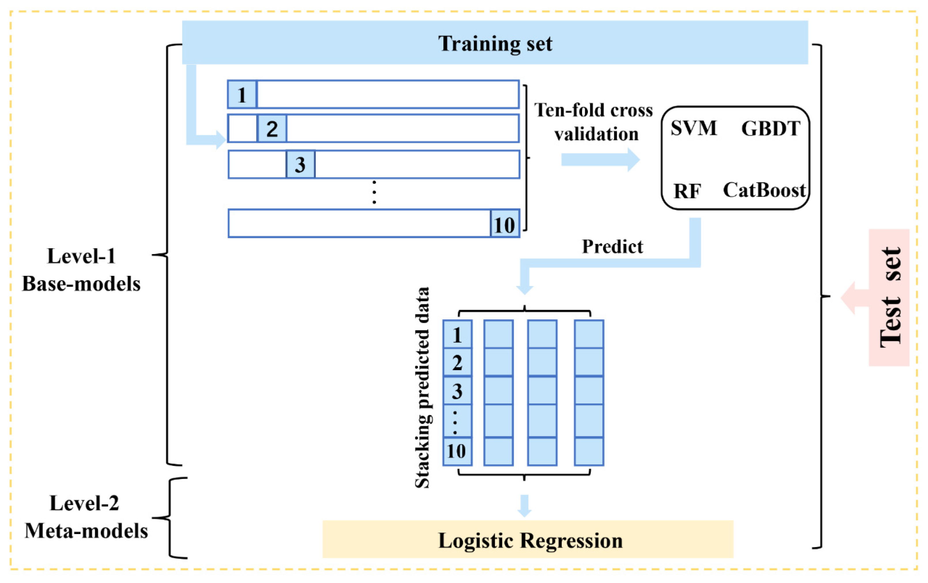
2.4.1. Modeling Techniques

SVM (support vector machine) is a popular supervised classification and regression learning technology based on structural risk minimization [38]. It is famous for robust generalization performance. It is by nature a binary classifier, but it can be extended for multiclass classification by “one-against-all” (ovr) or “one-against-one” (ovo) strategies. SVM with radial basis function (RBF) is favored in DSM [5]. Thus, it was used in the current study. Two parameters need to be defined for the RBF kernel: penalty cost (c) and kernel width (gamma).
RF (random forest) is a typical tree-based ensemble machine-learning technique via the bagging strategy. This algorithm has powerful scalability in big data and includes reasonable tolerance towards noise and outliers [39]. Two parameters should be adjusted for the RF model: the number of trees (n_estimators) and the number of features randomly sampled at each split (max_features).
GBDT (gradient-boosting decision tree) is an iterative optimization algorithm based on the regression decision tree. Each iteration fits a decision to the residuals left by the previous and then the prediction is accomplished by combining all trees [40]. Parameters, including the number of trees (n_estimators), the step size while learning (learning rata), depth of tree (max_depth), and subsample need to be defined for this algorithm.
CatBoost (categorical boosting) is a new ML algorithm proposed by Yandex Company. This ML approach makes improvements to the traditional GBDT algorithm. It can handle categorical features well based on greedy target-based statistics (Greedy TBS) [41]. Meanwhile, it overcomes the gradient bias problem and thus enhances the generalization ability of the model. Three key parameters: the number of trees (n_estimators), the step size while learning (learning rata), and the depth of the tree (max_depth) are defined in the current study.
The super learner applies the stacked generalization concept using out-of-fold predictions during the k-fold cross-validation process [13]. In short, it is a convex weighted combination of multiple ML algorithms (base learners). The four models mentioned above were used as base models to construct the super learner in the current work. The logistical regression was used as the meta-learner, which is a typical linear model. The building process of the super learner is shown in Figure 4: (1) dividing training and test sets; (2) splitting the training dataset ten-fold; (3) training the four base classifiers with ten-fold cross-validation and storing the out-of-fold predictions; (4) fitting a meta-model on the out-of-fold predictions and obtaining the weights of the base classifiers; (5) evaluating the performance based on the test set.

2.4.2. Model Evaluation

For each dataset, approximately 70% of the samples were randomly selected as the training sets and the remainder as the test sets. GridSearch-CV module was used to search optimal parameters based on the training set. The results of parameter optimization are shown in Supplementary Materials Table S1. The model performance was evaluated based on the independent test set. The evaluation indicators included OA, kappa, precision, recall rate, and F1-score. The relevant formulas are as follows:
O A = TP + TN TP + TN + FN + FP
K a p p a = OA P e 1 P e
R e c a l l   r a t e = TP TP + FN
P r e c i s o n = TP TP + FP
F 1 s c o r e = 2 × Precison × Recall Preciison + Recall
where TP, TN, FP, and FN are true positive, true negative, false positive, and false negative, respectively. P e is the probability of agreement when two classes are unconditionally independent.
Models with higher values of these indicators perform better. The model performance indicated by Kappa is: <0, poor; 0.00–0.20, slight; 0.21–0.40, fair; 0.41–0.60, moderate; 0.61–0.80, substantial; and 0.81–1.00, almost perfect [42].

2.4.3. Model Interpretation

The SHAP method proposed by Lundberg and Lee [25] provided a uniform interpretation framework for complex ML algorithms. This post hoc analysis method estimates the contribution of the individual variable by comparing the performance of the model with and without this variable. The contribution of the variable is characterized by the Shapley value based on the coalitional game theory [43]. The SHAP method is expressed as:
g ( z ) = 0 + i = 1 M i z i
where z { 0 , 1 } M denotes the presence or absence of a variable, M is the number of variables in the model, and 0 represents the constant value when all inputs are missing. i represents the contribution of variable i , i.e., the Shapley values. In the current work, SHAP library v37.0 was used to explain model outputs.

3. Results

3.1. Spectral Information Description and Variables Selection

Figure 5 shows the multispectral bands and vegetation indices of the soil samples with different textual classes, which were extracted from Sentinel-2 and Landsat-8 images. The spectral waveforms were similar between the two satellite sensors for consistent bands (blue, green, red, and NIR) and vegetation indices (NDVI, SAVI, EVI). The unique red-edge parameters of Sentinel-2 offered additional information. The reflectance of all bands and vegetation indices expressed the strong variation in different time phases owing to vegetation coverage change and crop rotation. Moreover, the distinction of spectral signals among the soil texture classes is shown in Figure 5. The Kruskal–Wallis test further confirmed this significant difference. Thus, valuable information from multitemporal optical images was useful for identifying soil texture class.
Approximately 14, 15, 33 spectral variables were retained for Dataset A, Dataset B, and Dataset C, respectively, after eliminating redundancy and multicollinearity among these covariates using VIF (Supplementary Materials Table S2). The optimized variables subsets differed with datasets because of the inherent discrepancy of sensors in spatial resolution, band numbers, and spectral range. Meanwhile, the results showed that single-band (blue and NIR bands) tended to be retained for traditional spectral indicators (VIR-NIR bands, NDVI, SAVI, and EVI), while derivative red-edge vegetation indices, including more unique explanatory power than single red-edge bands, were reserved for red-edge parameters (B5, B6, B7, S2REP, MCARI, IRECI, and MTCI). In addition, the number of the selected variables under different time phases was similar, indicating that the multitemporal remote sensing images could synthesize the surface coverage information in different periods to map soil properties.

3.2. Model Evaluation and Comparison

Figure 6 displays the performance of models with three datasets using five ML modeling techniques at three modeling resolutions. The results showed that the choice of sensors, modeling resolutions, and techniques affected the classification accuracy.
Models built by Datasets A and B, including consistent remote-sensed variables individually acquired from Landsat-8 and Sentinel-2, showed similar levels of soil texture classification under the same modeling resolution and technique. The best-performing models in explaining the variation of soil texture class were all based on Dataset C, which was derived from Sentinel-2 data with red-edge parameters. The average OA, kappa, precision, recall, and F1-score of the models with Dataset C were 3.4 and 3.0, 5.2 and 4.9, 3.5 and 3.5, 3.5 and 3.4, and 3.5 and 3.6% higher than that of others with Dataset A and Dataset B, respectively. These indicated the performance gap between the two sensors caused by the available spectral channels and proved the effectiveness of red-edge parameters from Sentinel-2 in identifying soil texture class.
Clearly, model performance varied with modeling resolutions. These models using different datasets achieved the best performance at 10 or 30 m resolution, and the classification accuracy of all models decreased when the modeling resolution changed from 30 to 60 m. For example, SVMs using Dataset A and Dataset B obtained the highest accuracy at 10 m, and their OA dropped from 0.7810 to 0.7743 and from 0.7920 to 0.7677, respectively, and Kappa reduced from 0.6941 to 0.6701 and from 0.6867 to 0.6512, with the modeling resolution from 30 m to 60 m. The super learner with Dataset C was best at 30 m with OA of 0.8429 and Kappa of 0.7964, but worst at 60 m with OA of 0.7964 and Kappa of 0.7113. Overall, the models usually performed better at fine and medium modeling resolutions than at coarse resolutions.
Compared with base classifiers, the super learner presented superior prediction accuracy. For instance, the highest accuracy was achieved by super learner, followed by CatBoost, GBDT, SVM, and RF techniques when identifying the soil texture class using Dataset A at 30 m resolution. The super learner consistently ranked first among these techniques based on any evaluation indicator, regardless of the datasets and modeling resolutions. In addition, the performance of four base classifiers changed with datasets and modeling resolutions. For example, SVM offered higher accuracy than RF and GBDT using Datasets A, B, and C at 10 m resolution, while the latter two methods performed better than SVM using Dataset C at 60 m resolution. CatBoost showed more robust performance than other base learners at 30 and 60 m resolution.
In addition, one-way ANOVA (Supplementary Materials Tables S3–S5) was performed for testing significant differences in classification results among datasets, modeling resolutions, and modeling techniques.
Figure 7 reveals the concrete classification results of sandy, loamy, and clayey soils using the F1-score. The models’ ability to differentiate each soil texture class varied significantly among sensors, modeling resolutions, and modeling techniques. For example, the F1-score of the super learner using Dataset A at 30 m was 0.975, 0.679, and 0.716 for sandy, loamy, and clayey soils, respectively, and using Dataset B at 30 m was 0.963,0.681, 0.744. The above model with Sentinel-2 data obtained slightly higher precision in separating loamy and clayey soils than that with Landsat-8 data, whereas the latter had the advantage in identifying sandy soils. However, the opposite is true at 60 m. Nevertheless, consistent trends were observed in all models. On the one hand, sandy soils were easily distinguished, with an F1-score above 0.9. On the other hand, the gain from the sensors, modeling resolutions, and modeling techniques in identifying loamy soils was prominent. For instance, because of the addition of red-edge parameters, the improvement in the F1-score of RF with Dataset C over that with Dataset B was 2.3, 2.9, and 5.2% for sandy, loamy, and clayey soils at 10 m, respectively, 4.5, 11.2, 3.6% at 30 m, 2.5, 5.8, and 0.8% at 60 m. Confusion matrices in Supplementary Materials Figure S1 show more details about the classification results.

3.3. Variable Importance

The best model (the super learner using Dataset C at 30 m) was employed to analyze the importance of individual variables. In this case, the relative weights of four base learners of the super learner were 34.12 (SVM), 30.59 (CatBoost), 23.89 (RF), and 11.41% (GBDT), respectively.
The variables ranking based on the SHAP technique is presented in Figure 8. Overall, the red-edge factor MCARI in August (MACARI_Aug) was the most essential explanatory covariate for soil texture classification, followed by NDVI in August (NDVI_Aug) and Blue band in December (Blue_Dec) with mean absolute values of SHAP of 0.1930 and 0.1369, respectively (Figure 8a). Additionally, the local contribution of individual variables for each soil textural class also was displayed (Figure 8b–d). The key variables with high relative importance were MCARI_Aug (9.36%) > Blue_Dec (8.16%) > Blue band in August (Blue_Aug, 6.40%) for sandy soils, MCARI_Aug (12.24%) > NDVI_Aug (7.70%) > NIR band in September (NIR_Sep, 4.78%) for loamy soils, NDVI_Aug (13.66%) > Blue_Dec (7.92%) > NDVI in December (NDVI_Dec,7.66%) for clayey soils. Meanwhile, the results indicated that August was the optimum period to identify three different soil texture classes.

3.4. Spatial Distribution of Soil Texture Class

The map of soil texture classification is produced based on the best model and the spatial pattern of soil texture class is shown in Figure 9. Sandy soils were scattered in northeast and southwest areas, loamy soils concentrated in the northern part, and clayey soils mainly located in south and west regions. The percentages of sandy, loamy, and clayey soils were 2, 66, and 32%, respectively, over the dry farmland.

4. Discussion

4.1. The Potential of Multitemporal Remote Sensing Data for Predicting Soil Properties

The rapid development of remote sensing techniques provides great prospects for mapping soil properties. Numerous research studies have demonstrated the effectiveness of remote sensing data in predicting soil attributes [1,3,44]. Some of them combined optical images with other auxiliary data for explaining the variability of soil properties at various scales, focusing on the added value of satellite products applied for DSM; some aimed at exploring the feasibility of multispectral images in describing the spatial distribution of various properties of bare soil [11,12]. Our study evaluated the capabilities of purely multitemporal optical images in predicting soil properties for densely vegetated regions, exploring more possibilities of satellite images in DSM. The results showed that multitemporal optical images had strong potential in identifying soil texture class under vegetation cover. In fact, soil texture classes influence the availability of soil moisture, heat capacity, transport of solutes, and other soil properties, which lead to the different spectral responses of vegetation characteristics [45]. In turn, this heterogeneity from vegetation spectral signals could be retrieved by satellites and then be accumulated in multitemporal optical data, which is sufficient to discrete different vegetation characteristics and their related soil attributes (soil texture). Therefore, multitemporal optical images could characterize vegetation growth and development and then infer soil properties [46], which may be promising for DSM.
Supplementary Materials Table S6 shows the performance of six super learner models using the mono-temporal Sentinel-2 image involving red-edge parameters at 30 m. Their predictive accuracies varied with vegetation covers and were much lower than that of the model using multitemporal images. Compared with mono-temporal satellite images, multitemporal remote sensing data could provide more valuable auxiliary information for soil property prediction [47]. Similarly, Maynard and Levi [45] noted that increasing the temporal frequency of remote sensing images could greatly improve the predictive performance of soil mapping models (Supplementary Materials Figure S2). Meanwhile, the results based on both mono-temporal and multi-temporal predictions indicated that August was a suitable temporal phase to distinguish soil textural classes. The densely vegetated images could provide useful information for remote monitoring.

4.2. The Performance Comparison of Models Based on Different Sensors, Modeling Resolutions, and Modeling Techniques

Multispectral satellites are essential and effective data sources for predicting soil properties at various scales [1,48,49,50]. The current study compared the performance of models based on different multispectral satellites (Sentinel-2 and Landsat-8) using retrieved vegetation properties as proxies of soil properties. The results indicated that the inherent differential structure of sensors caused their performance gap in separating soil textures. Sentinel-2 has more available spectral channels and derived spectral indices (red-edge parameters) than Landsat-8. When these unique parameters were added, the classification accuracies of Sentinel-2 models were substantially improved and were much higher than that of Landsat-8 models, especially in identifying loamy soils. Additionally, the results of the variable importance ranking indicated that the contribution of red-edge parameters exceeded that of traditional spectral indices. The red edge lies between the red and NIR portions of the electromagnetic spectrum, and the increase of reflectance within this range is the most universal and sensitive spectral response of plants to stress [51,52]. Previous studies have emphasized the usefulness of this spectral domain in estimating LAI [53], plant chlorophyll content [54], and nitrogen uptake [8]. Moreover, some scholars confirmed that Sentinel-2 with red-edge parameters produced better accuracy statistics by comparing different optical images in the fields of land cover [55], crop identification [56], and biological mapping [57]. Thus, the red-edge parameters, having powerful availability in the vegetation remote sensing community, may capture more detailed and valuable vegetation signals as proxies for inferring soil properties. Similar findings are also reported that red-edge bands of Sentinel-2 images provided a good correlation with clay content under bare soils [10]. Silvero et al. [48] obtained an opposite conclusion in mapping various topsoil properties based on Sentinel-2 and Landsat-8 bare soil images in Brazil. They found that the use of red-edge bands from Sentinel-2 did not bring large gains in model performance while multi-temporal images from Landsat-8 offered the best prediction performance. The availability of red-edge parameters of Sentinel-2 needs to be proved in more regions with different management modes, climate conditions, and vegetation cover conditions.
Different from some studies using single modeling resolution, our predictive models were conducted at multiple spatial scales. We found that these models using satellite products had diverse predictive capabilities for soil properties at different modeling resolutions. The ideal classification accuracies were usually obtained at fine and medium modeling resolutions (10 or 30 m), whereas the performances of these models were poor at coarse resolutions (60 m) in this study. This is closely related to the spatial distribution of soil texture class in the study area. Specifically, the proportion of sandy soil is small and its distribution is discontinuous (Figure 9). Most sandy soils are scattered in loamy or clayey soils. Therefore, the real spectral information characterizing sandy soils in a short distance could be largely retrieved at fine and medium resolutions, while coarser modeling resolution exacerbates the mixed-pixel problem, influencing the spectral characteristics of sandy soils. Finally, the overall accuracy of the model will decrease due to the misclassification of sandy soils (Supplementary Materials Figure S1). Meanwhile, it was also found that the performances of models based on satellite products at medium resolutions were competitive and even superior to fine resolutions. This is not strange. Cavazzi et al. [58] pointed out that more exhaustive covariates may be “noise” that degrades the predictions due to an excess of detail. This could explain our results that these optical images at 10 m resolution may retrieve smaller objects (e.g., individual plants) with highly variable spectral behavior, adding noise to the correlation between satellite and soil properties. At the same time, optical data at medium modeling resolution usually capture collections of objects, and thus their variations were smoothed out in the pixel, reducing noise [59]. Quantitative assessment based on multiple modeling resolutions showed comprehensive insights into predicting soil properties [60]. Although it is widely known that the spatial scale of input variables significantly influences predictive accuracy, most DSM research studies are still performed at a single spatial scale [38]. Therefore, we recommend selecting the optimal modeling resolution for input variables by constructing multiscale predictive models. This may be beneficial for predicting some target soil properties.
Modeling techniques also significantly influenced the predictive accuracy in the current study. RF, SVM, and GBDT are the primary methods for solving learning problems with heterogeneous characteristics, noisy data, and complex dependencies during the past decades. In DSM, they are always favored and their predictive performances are often compared. However, the performance ranking of these algorithms changes with soil properties, study area, and datasets. CatBoost is a novel gradient-boosting technology [61]. This ML approach makes improvements in parallelism based on the traditional GBDT algorithm, greatly reducing layout time and being easier to implement. Moreover, it shows better accuracy and lower computational costs than SVM and other tree ensemble classifiers (e.g., RF, GBDT, XGBoost) in crop evapotranspiration estimation [41,62], electric theft detection [63] and atmospheric PM2.5 forecasting [64]. However, it is rarely applied in soil properties mapping. Our study showed that CatBoost offered higher precision than RF, SVM, and GBDT in the identification of soil textural class in most cases. Nevertheless, none has been found to consistently outperform others in the current study. Therefore, it is necessary to calibrate and evaluate competitive modeling techniques based on specific experimental datasets at different modeling resolutions [5]. The super learner, integrating the strengths of the four learners above, presented the best and most robust performance in any case. Similarly, recent studies [65,66,67] evaluated the efficacy of this ensemble model in DSM. Taghizadeh-Mehrjardi et al. [13] applied the super learner approach that combined 12 ML models to predict various soil properties in Iran. They pointed out the super learner had higher accuracy than the individual base learners. Tan et al. [66] assessed the distribution trend of soil heavy metal (pb) in mining areas based on this stacking strategy. They presented a considerable outcome obtained by the ensemble learning method with the highest R2 (0.71) and lowest RMSE (4.03 mg/kg). However, Somarathna et al. [67] reported that combing the ML algorithms could not give significant improvement (~2%) in soil property prediction, although it may be superior to the individual base models. They stressed that ensemble models could only offer benefits when integrating diverse ML algorithms, covariates, or datasets. That is, the reasonable results generated by the stacking strategy depend on the diversity in individual models. The most improvement could be obtained in super learner only when the predictive value from base learners are less correlated [68]. However, selecting a combination of dissimilar models is not always an easy practice because of the expensive computational cost. Therefore, the choice of model techniques needs comprehensive consideration.

4.3. The Interpretability of the Super Learner

Although the usability of the super learner has been confirmed in some studies, its interpretability has rarely been explored. Unlike tree models with inherent feature importance rankings, the super learner based on the stacking concept cannot explicitly quantify the contribution of individual predictors. A novel technique (SHAP) was introduced to explain the super learner. This approach evaluated the local contribution of individual variables as well as global importance (Figure 8). Moreover, it also thoroughly displayed the decision progress of the super learner (Figure 10). The red-edge parameter MCARI_Aug was the key variable in separating loamy and sandy soils (Figure 10a,b). As the value of MCARI_Aug increased (the dot color transition from blue to red), the probability of being predicted as sandy texture increased (SHAP values change from negative to positive, Figure 10a), and the probability of being loamy texture decreased (Figure 10b). The result was consistent with our prior knowledge. Specifically, the agricultural land over the study area is shaded by sweet potato leaves in August, and sweet potato as a tuber crop is sensitive to soil texture classes [69]. Huang [70] reported that sandy soils are suitable for tuber crops because they are loose and porous with good aeration and significant differences in temperature between day and night. MCARI has a clear response to plant chlorophyll content [71], indicating the development status and growth vitality of vegetation [72]. Therefore, sandy soils had higher values of MCARI_Aug than loamy soils, indicating that sandy soils were better for sweet potatoes than loamy soils. The magnitude, prevalence, and direction of other variable effects on sandy, loamy, and clayey textures were also deduced according to visualization of the SHAP method. The method improves the trustworthiness of the complex model, providing promising support for ML-assisted tasks in DSM.

4.4. Deficiencies and Prospects

The current study quantified the effects of sensors, modeling resolutions, and modeling techniques on soil texture classification. Although the soil texture classification map successfully explained the variation of soil texture class in this area, there were several limitations. Firstly, this study was performed on the small spatial scale (small basin), which limited the investigation of the feasibility of coarser modeling resolutions and satellites products without fine spatial resolutions in DSM. For relevant research studies on soil property prediction in larger areas, more diverse sensors and modeling resolutions should be considered. In particular, the European Space Agency (ESA) recently launched Sentinel-3 satellites. They have 21 spectral bands (400–1020 nm), 300 m spatial resolution, and a short revisit time of fewer than 2 days. Moreover, they performed relatively well as a single data source for SOC mapping at the national scale [73]. Therefore, it is necessary to explore the effectiveness of more satellite products and modeling resolutions for DSM in larger regions, which will provide comprehensive insights for effective modeling of soil properties on various scales using different satellite products.
In addition, this study focused on exploring the possibility of multitemporal optical images in DSM by using retrieved vegetation attributes as proxies of soil properties, while synthetic aperture radar (SAR) data and some traditional environment auxiliary data (e.g., DEM, geological map) were not used. Different from optical images, SAR data have the advantages of all-weather, day, and night imaging, and their backscattering coefficient can provide information beyond the vegetative cover and the soil surface [74]; traditional environment auxiliary variables are closely related to soil formation and development, having important influences on soil properties modeling. Although their individual abilities to predict soil properties were not as prominent as those of optical images [4,75,76,77], some studies indicated that the combination of these data and optical images produced the most accurate prediction of soil properties in complex landscapes [75]. Future research is needed to examine the added benefit of incorporating multisource data into soil prediction models using various modeling resolutions at large scales.

5. Conclusions

This work investigated the feasibility of multitemporal remote sensing data from different satellites in mapping soil texture class using retrieved vegetation properties as proxies of soil properties. The influences of sensors, modeling resolutions, and modeling techniques on soil texture classification were further explored. The SHAP technique was introduced to interpret the model outputs. Our conclusions can be summarized as follows:
(1) It is feasible to identify soil textural class purely using multi-temporal remote sensing data under vegetation cover, which provided acceptable performance with OA between 0.7677 and 0.8451, kappa between 0.6505 and 0.7673, precision between 0.76 and 0.8394, recall between 0.7610 and 0.8410, and an F1-score between 0.7605 and 0.8398.
(2) The choice of sensors, modeling resolutions, and modeling techniques significantly affected the outputs. Sentinel-2 has more of an advantage than Landsat-8, in particular, its red-edge parameters, which bring more valuable information for identifying soil texture class. Better classification accuracies were usually obtained at fine and medium modeling resolutions than at coarse resolutions. The super learner presented higher precision consistently when compared with base models, and this strategy may be promising for mapping soil properties.
(3) SHAP is a powerful tool for interpreting ML algorithms with black box properties. It gives visual representations of the decision processes of ML models, improving the trustworthiness of these models.

Supplementary Materials

The following supporting information can be downloaded at: https://www.mdpi.com/article/10.3390/rs14215571/s1, Figure S1: Confusion matrices based on three dataset using super learner at three spatial resolutions; Figure S2: Accuracy indicators change with number of spectral images; Table S1: The results of parameter optimization; Table S2: Variance inflation factors (VIF) of remote sensing covariates are used to identify soils texture class in different datasets; Table S3: Analysis of variance of classification results for datasets; Table S4: Analysis of variance of classification results for modelling resolutions; Table S5: Analysis of variance of classification results for modelling techniques; Table S6: Performance evaluation of six super learner models using mono-temporal Sentinel-2 image involving red-edge parameters at 30 m.

Author Contributions

Conceptualization, methodology, software, and writing—original draft, Y.Z.; writing—review and editing, W.W.; supervision, H.L. All authors have read and agreed to the published version of the manuscript.

Funding

This research received no external funding.

Conflicts of Interest

The authors declare no conflict of interest.

References

  1. Loiseau, T.; Chen, S.; Mulder, V.L.; Dobarco, M.R.; Richer-De-Forges, A.C.; Lehmann, S.; Bourennane, H.; Saby, N.P.A.; Martin, M.P.; Vaudour, E.; et al. Satellite data integration for soil clay content modelling at a national scale. Int. J. Appl. Earth Obs. Geoinf. 2019, 82, 101905. [Google Scholar] [CrossRef]
  2. Vaudour, E.; Gomez, C.; Fouad, Y.; Lagacherie, P. Sentinel-2 image capacities to predict common topsoil properties of temperate and Mediterranean agroecosystems. Remote Sens. Environ. 2019, 223, 21–33. [Google Scholar] [CrossRef]
  3. Wu, W.; Yang, Q.; Lv, J.; Li, A.; Liu, H. Investigation of remote sensing imageries for identifying soil texture classes using classification methods. IEEE Trans. Geosci. Remote Sens. 2019, 57, 1653–1663. [Google Scholar] [CrossRef]
  4. Zhou, Y.; Wu, W.; Wang, H.; Zhang, X.; Yang, C.; Liu, H. Identification of Soil Texture Classes Under Vegetation Cover Based on Sentinel-2 Data with SVM and SHAP Techniques. IEEE J. Sel. Top. Appl. Earth Obs. Remote Sens. 2022, 15, 3758–3770. [Google Scholar] [CrossRef]
  5. Zhou, T.; Geng, Y.; Ji, C.; Xu, X.; Wang, H.; Pan, J.; Bumberger, J.; Haase, D.; Lausch, A. Prediction of soil organic carbon and the C:N ratio on a national scale using machine learning and satellite data: A comparison between Sentinel-2, Sentinel-3 and Landsat-8 images. Sci. Total Environ. 2021, 755, 142661. [Google Scholar] [CrossRef] [PubMed]
  6. Poggio, L.; Gimona, A. 3D mapping of soil texture in Scotland. Geoderma Reg. 2017, 9, 5–16. [Google Scholar] [CrossRef]
  7. Falahatkar, S.; Hosseini, S.M.; Ayoubi, S.; Salmanmahiny, A. Predicting soil organic carbon density using auxiliary environmental variables in northern Iran. Arch. Agron. Soil Sci. 2016, 62, 375–393. [Google Scholar] [CrossRef]
  8. Zhang, Y.; Sui, B.; Shen, H.; Ouyang, L. Mapping stocks of soil total nitrogen using remote sensing data: A comparison of random forest models with different predictors. Comput. Electron. Agric. 2019, 160, 23–30. [Google Scholar] [CrossRef]
  9. Zhou, T.; Geng, Y.; Chen, J.; Pan, J.; Haase, D.; Lausch, A. High-resolution digital mapping of soil organic carbon and soil total nitrogen using DEM derivatives, Sentinel-1 and Sentinel-2 data based on machine learning algorithms. Sci. Total Environ. 2020, 729, 138244. [Google Scholar] [CrossRef]
  10. Gholizadeh, A.; Žižala, D.; Saberioon, M.; Borůvka, L. Soil organic carbon and texture retrieving and mapping using proximal, airborne and Sentinel-2 spectral imaging. Remote Sens. Environ. 2018, 218, 89–103. [Google Scholar] [CrossRef]
  11. Chagas, C.D.S.; Junior, W.D.C.; Bhering, S.B.; Filho, B.C. Spatial prediction of soil surface texture in a semiarid region using random forest and multiple linear regressions. CATENA 2016, 139, 232–240. [Google Scholar] [CrossRef]
  12. Gallo, B.C.; Demattê, J.A.M.; Rizzo, R.; Safanelli, J.L.; Mendes, W.D.S.; Lepsch, I.F.; Sato, M.V.; Romero, D.J.; Lacerda, M.P.C. Multi-Temporal Satellite Images on Topsoil Attribute Quantification and the Relationship with Soil Classes and Geology. Remote Sens. 2018, 10, 1571. [Google Scholar] [CrossRef]
  13. Taghizadeh-Mehrjardi, R.; Hamzehpour, N.; Hassanzadeh, M.; Heung, B.; Goydaragh, M.G.; Schmidt, K.; Scholten, T. Enhancing the accuracy of machine learning models using the super learner technique in digital soil mapping. Geoderma 2021, 399, 115108. [Google Scholar] [CrossRef]
  14. Davis, E.; Wang, C.; Dow, K. Comparing Sentinel-2 MSI and Landsat 8 OLI in soil salinity detection: A case study of agricultural lands in coastal North Carolina. Int. J. Remote Sens. 2019, 40, 6134–6153. [Google Scholar] [CrossRef]
  15. Guo, L.; Sun, X.; Fu, P.; Shi, T.; Dang, L.; Chen, Y.; Linderman, M.; Zhang, G.; Zhang, Y.; Jiang, Q.; et al. Mapping soil organic carbon stock by hyperspectral and time-series multispectral remote sensing images in low-relief agricultural areas. Geoderma 2021, 398, 115118. [Google Scholar] [CrossRef]
  16. Zhang, Y.; Guo, L.; Chen, Y.; Shi, T.; Luo, M.; Ju, Q.; Zhang, H.; Wang, S. Prediction of soil organic carbon based on Landsat 8 monthly NDVI data for the Jianghan Plain in Hubei Province, China. Remote Sens. 2019, 11, 1683. [Google Scholar] [CrossRef] [Green Version]
  17. Mulder, V.; Lacoste, M.; Richer-De-Forges, A.; Arrouays, D. GlobalSoilMap France: High-resolution spatial modelling the soils of France up to two meter depth. Sci. Total Environ. 2016, 573, 1352–1369. [Google Scholar] [CrossRef]
  18. Lin, C.; Zhu, A.-X.; Wang, Z.; Wang, X.; Ma, R. The refined spatiotemporal representation of soil organic matter based on remote images fusion of Sentinel-2 and Sentinel-3. Int. J. Appl. Earth Obs. Geoinf. ITC J. 2020, 89, 102094. [Google Scholar] [CrossRef]
  19. Wang, J.; Ding, J.; Yu, D.; Ma, X.; Zhang, Z.; Ge, X.; Teng, D.; Li, X.; Liang, J.; Guo, Y.; et al. Machine learning-based detection of soil salinity in an arid desert region, Northwest China: A comparison between Landsat-8 OLI and Sentinel-2 MSI. Sci. Total. Environ. 2020, 707, 136092. [Google Scholar] [CrossRef]
  20. Miller, B.A.; Koszinski, S.; Wehrhan, M.; Sommer, M. Impact of multi-scale predictor selection for modeling soil properties. Geoderma 2015, 239–240, 97–106. [Google Scholar] [CrossRef]
  21. Liu, L.; Ji, M.; Buchroithner, M. Combining partial least squares and the gradient-boosting method for soil property retrieval using visible near-infrared shortwave infrared spectra. Remote Sens. 2017, 9, 1299. [Google Scholar] [CrossRef] [Green Version]
  22. Samat, A.; Li, E.; Du, P.; Liu, S.; Xia, J. GPU-accelerated catboost-forest for hyperspectral image classification via parallelized mRMR ensemble subspace feature selection. IEEE J. Sel. Top. Appl. Earth Obs. Remote Sens. 2021, 14, 3200–3214. [Google Scholar] [CrossRef]
  23. Wyss, R.; Schneeweiss, S.; Van Der Laan, M.; Lendle, S.D.; Ju, C.; Franklin, J.M. Using super learner prediction modeling to improve high-dimensional propensity score estimation. Epidemiology 2018, 29, 96–106. [Google Scholar] [CrossRef] [PubMed]
  24. Breiman, L. Stacked regressions. Mach. Learn. 1996, 24, 49–64. [Google Scholar] [CrossRef] [Green Version]
  25. Lundberg, S.M.; Lee, S.-I. A Unified Approach to Interpreting Model Predictions. Proc. Adv. Neural Inf. Process. Syst. 2017, 30, 4765–4774. [Google Scholar]
  26. Guo, Y.; Ma, W.; Li, J.; Liu, W.; Qi, P.; Ye, Y.; Guo, B.; Zhang, J.; Qu, C. Effects of microplastics on growth, phenanthrene stress, and lipid accumulation in a diatom, Phaeodactylum tricornutum. Environ. Pollut. 2020, 257, 113628. [Google Scholar] [CrossRef]
  27. Xu, J.; Saleh, M.; Hatzopoulou, M. A machine learning approach capturing the effects of driving behaviour and driver characteristics on trip-level emissions. Atmos. Environ. 2020, 224, 117311. [Google Scholar] [CrossRef]
  28. Mangalathu, S.; Hwang, S.-H.; Jeon, J.-S. Failure mode and effects analysis of RC members based on machine-learning-based SHapley Additive exPlanations (SHAP) approach. Eng. Struct. 2020, 219, 110927. [Google Scholar] [CrossRef]
  29. Jahn, R.; Blume, H.P.; Asio, V.B.; Spaargaren, O.; Schad, P. Guidelines for Soil Description; FAO: Rome, Italy, 2006. [Google Scholar]
  30. Richer-de-Forges, A.C.; Arrouays, D.; Chen, S.; Dobarco, M.R.; Libohova, Z.; Roudier, P.; Minasny, B.; Bourennane, H. Hand-feel soil texture and particle-size distribution in central France. Relationships and implications. Catena 2022, 213, 106155. [Google Scholar] [CrossRef]
  31. Pachepsky, Y.; Rawls, W.; Lin, H. Hydropedology and pedotransfer functions. Geoderma 2006, 131, 308–316. [Google Scholar] [CrossRef]
  32. Vos, C.; Don, A.; Prietz, R.; Heidkamp, A.; Freibauer, A. Field-based soil-texture estimates could replace laboratory analysis. Geoderma 2016, 267, 215–219. [Google Scholar] [CrossRef]
  33. Soil Science Division Staff. Soil survey manual. USDA Handb. 2017, 18, 639. [Google Scholar]
  34. Wang, S.; Liu, S.; Zhang, J.; Che, X.; Yuan, Y.; Wang, Z.; Kong, D. A new method of diesel fuel brands identification: SMOTE oversampling combined with XGBoost ensemble learning. Fuel 2020, 282, 118848. [Google Scholar] [CrossRef]
  35. Taghizadeh-Mehrjardi, R.; Schmidt, K.; Eftekhari, K.; Behrens, T.; Jamshidi, M.; Davatgar, N.; Toomanian, N.; Scholten, T. Synthetic resampling strategies and machine learning for digital soil mapping in Iran. Eur. J. Soil Sci. 2020, 71, 352–368. [Google Scholar] [CrossRef]
  36. Johnson, B.A.; Iizuka, K. Integrating OpenStreetMap crowdsourced data and Landsat time-series imagery for rapid land use/land cover (LULC) mapping: Case study of the Laguna de Bay area of the Philippines. Appl. Geogr. 2016, 67, 140–149. [Google Scholar] [CrossRef]
  37. Zeraatpisheh, M.; Garosi, Y.; Owliaie, H.R.; Ayoubi, S.; Taghizadeh-Mehrjardi, R.; Scholten, T.; Xu, M. Improving the spatial prediction of soil organic carbon using environmental covariates selection: A comparison of a group of environmental covariates. Catena 2022, 208, 105723. [Google Scholar] [CrossRef]
  38. Forkuor, G.; Hounkpatin, O.K.L.; Welp, G.; Thiel, M. High resolution mapping of soil properties using remote sensing variables in south-western Burkina Faso: A comparison of machine learning and multiple linear regression models. PLoS ONE 2017, 12, e0170478. [Google Scholar] [CrossRef] [Green Version]
  39. Yang, L.; He, X.; Shen, F.; Zhou, C.; Zhu, A.-X.; Gao, B.; Chen, Z.; Li, M. Improving prediction of soil organic carbon content in croplands using phenological parameters extracted from NDVI time series data. Soil Tillage Res. 2020, 196, 104465. [Google Scholar] [CrossRef]
  40. Yang, L.; Mansaray, L.R.; Huang, J.; Wang, L. Optimal segmentation scale parameter, feature subset and classification algorithm for geographic object-based crop recognition using multisource satellite imagery. Remote Sens. 2019, 11, 514. [Google Scholar] [CrossRef] [Green Version]
  41. Zhang, Y.; Zhao, Z.; Zheng, J. CatBoost: A new approach for estimating daily reference crop evapotranspiration in arid and semi-arid regions of Northern China. J. Hydrol. 2020, 588, 125087. [Google Scholar] [CrossRef]
  42. Landis, J.R.; Koch, G.G. The Measurement of Observer Agreement for Categorical Data. Biometrics 1977, 33, 159–174. [Google Scholar] [CrossRef] [PubMed] [Green Version]
  43. Shapley, L.S. A value for n-person games. In Theory of Games; Princeton University Press: Princeton, NJ, USA, 1953; pp. 307–317. [Google Scholar]
  44. Ceddia, M.B.; Gomes, A.S.; Vasques, G.M.; Pinheiro, E. Soil Carbon Stock and Particle Size Fractions in the Central Amazon Predicted from Remotely Sensed Relief, Multispectral and Radar Data. Remote Sens. 2017, 9, 124. [Google Scholar] [CrossRef]
  45. Maynard, J.J.; Levi, M.R. Hyper-temporal remote sensing for digital soil mapping: Characterizing soil-vegetation response to climatic variability. Geoderma 2017, 285, 94–109. [Google Scholar] [CrossRef] [Green Version]
  46. Zhang, L.; Cai, Y.; Huang, H.; Li, A.; Yang, L.; Zhou, C. A CNN-LSTM model for soil organic carbon content prediction with long time series of MODIS-based phenological variables. Remote Sens. 2022, 14, 4441. [Google Scholar] [CrossRef]
  47. Guo, L.; Fu, P.; Shi, T.; Chen, Y.; Zeng, C.; Zhang, H.; Wang, S. Exploring influence factors in mapping soil organic carbon on low-relief agricultural lands using time series of remote sensing data. Soil Tillage Res. 2021, 210, 104982. [Google Scholar] [CrossRef]
  48. Silvero, N.E.Q.; Demattê, J.A.M.; Amorim, M.T.A.; dos Santos, N.V.; Rizzo, R.; Safanelli, J.L.; Poppiel, R.R.; Mendes, W.D.S.; Bonfatti, B.R. Soil variability and quantification based on Sentinel-2 and Landsat-8 bare soil images: A comparison. Remote Sens. Environ. 2021, 252, 112117. [Google Scholar] [CrossRef]
  49. Castaldi, F.; Hueni, A.; Chabrillat, S.; Ward, K.; Buttafuoco, G.; Bomans, B.; Vreys, K.; Brell, M.; van Wesemael, B. Evaluating the capability of the Sentinel 2 data for soil organic carbon prediction in croplands. ISPRS J. Photogramm. Remote Sens. 2019, 147, 267–282. [Google Scholar] [CrossRef]
  50. Bartholomeus, H.; Kooistra, L.; Stevens, A.; van Leeuwen, M.; van Wesemael, B.; Ben-Dor, E.; Tychon, B. Soil Organic Carbon mapping of partially vegetated agricultural fields with imaging spectroscopy. Int. J. Appl. Earth Obs. Geoinf. 2011, 13, 81–88. [Google Scholar] [CrossRef]
  51. Carter, G.A.; Knapp, A.K. Leaf optical properties in higher plants: Linking spectral characteristics to stress and chlorophyll concentration. Am. J. Bot. 2001, 88, 677–684. [Google Scholar] [CrossRef] [Green Version]
  52. Eitel, J.U.H.; Vierling, L.A.; Litvak, M.E.; Long, D.S.; Schulthess, U.; Ager, A.A.; Krofcheck, D.J.; Stoscheck, L. Broadband, red-edge information from satellites improves early stress detection in a New Mexico conifer woodland. Remote Sens. Environ. 2011, 115, 3640–3646. [Google Scholar] [CrossRef]
  53. Asam, S.; Fabritius, H.; Klein, D.; Conrad, C.; Dech, S. Derivation of leaf area index for grassland within alpine upland using multi-temporal RapidEye data. Int. J. Remote Sens. 2013, 34, 8628–8652. [Google Scholar] [CrossRef]
  54. Clevers, J.G.P.W.; Gitelson, A.A. Remote estimation of crop and grass chlorophyll and nitrogen content using red-edge bands on Sentinel-2 and -3. Int. J. Appl. Earth Observ. Geoinf. 2013, 23, 344–351. [Google Scholar] [CrossRef]
  55. Forkuor, G.; Dimobe, K.; Serme, I.; Tondoh, J.E. Landsat-8 vs. Sentinel-2: Examining the added value of sentinel-2’s red-edge bands to land-use and land-cover mapping in Burkina Faso. GIScience Remote Sens. 2018, 55, 331–354. [Google Scholar] [CrossRef]
  56. Wolanin, A.; Camps-Valls, G.; Gómez-Chova, L.; Mateo-García, G.; van der Tol, C.; Zhang, Y.; Guanter, L. Estimating crop primary productivity with Sentinel-2 and Landsat 8 using machine learning methods trained with radiative transfer simulations. Remote Sens. Environ. 2019, 225, 441–457. [Google Scholar] [CrossRef]
  57. Astola, H.; Häme, T.; Sirro, L.; Molinier, M.; Kilpi, J. Comparison of Sentinel-2 and Landsat 8 imagery for forest variable prediction in boreal region. Remote Sens. Environ. 2019, 223, 257–273. [Google Scholar] [CrossRef]
  58. Cavazzi, S.; Corstanje, R.; Mayr, T.; Hannam, J.; Fealy, R. Are fine resolution digital elevation models always the best choice in digital soil mapping? Geoderma 2013, 195, 111–121. [Google Scholar] [CrossRef]
  59. Samuel-Rosa, A.; Heuvelink, G.B.M.; Vasques, G.M.; Anjos, L.H.C. Do more detailed environmental covariates deliver more accurate soil maps? Geoderma 2015, 243, 214–227. [Google Scholar] [CrossRef]
  60. Garosi, Y.; Ayoubi, S.; Nussbaum, M.; Sheklabadi, M. Effects of different sources and spatial resolutions of environmental covariates on predicting soil organic carbon using machine learning in a semi-arid region of Iran. Geoderma Reg. 2022, 29, e00513. [Google Scholar] [CrossRef]
  61. Dorogush, A.V.; Ershov, V.; Gulin, A. CatBoost: Gradient boosting with categorical features support. arXiv 2018, arXiv:1810.1136. [Google Scholar]
  62. Huang, G.; Wu, L.; Ma, X.; Zhang, W.; Fan, J.; Yu, X.; Zeng, W.; Zhou, H. Evaluation of CatBoost method for prediction of reference evapotranspiration in humid regions. J. Hydrol. 2019, 574, 1029–1041. [Google Scholar] [CrossRef]
  63. Hussain, S.; Mustafa, M.W.; Jumani, T.A.; Baloch, S.K.; Alotaibi, H.; Khan, I.; Khan, A. A novel feature engineered-CatBoost-based supervised machine learning framework for electricity theft detection. Energy Rep. 2021, 7, 4425–4436. [Google Scholar] [CrossRef]
  64. Ding, Y.; Chen, Z.; Lu, W.; Wang, X. A CatBoost approach with wavelet decomposition to improve satellite-derived high-resolution PM2. 5 estimates in Beijing-Tianjin-Hebei. Atmos. Environ. 2021, 249, 118212. [Google Scholar] [CrossRef]
  65. Das, B.; Rathore, P.; Roy, D.; Chakraborty, D.; Jatav, R.S.; Sethi, D.; Kumar, P. Comparison of bagging, boosting and stacking algorithms for surface soil moisture mapping using optical-thermal-microwave remote sensing synergies. Catena 2022, 217, 106485. [Google Scholar] [CrossRef]
  66. Tan, K.; Ma, W.; Chen, L.; Wang, H.; Du, Q.; Du, P.; Yan, B.; Liu, R.; Li, H. Estimating the distribution trend of soil heavy metals in mining area from HyMap airborne hyperspectral imagery based on ensemble learning. J. Hazard. Mater. 2021, 401, 123288. [Google Scholar] [CrossRef] [PubMed]
  67. Somarathna, P.; Minasny, B.; Malone, B.P. More data or a better model? Figuring out what matters most for the spatial prediction of soil carbon. Soil Sci. Soc. Am. J. 2017, 81, 1413–1426. [Google Scholar] [CrossRef]
  68. Taghizadeh-Mehrjardi, R.; Schmidt, K.; Amirian-Chakan, A.; Rentschler, T.; Zeraatpisheh, M.; Sarmadian, F.; Valavi, R.; Davatgar, N.; Behrens, T.; Scholten, T. Improving the spatial prediction of soil organic carbon content in two contrasting climatic regions by stacking machine learning models and rescanning covariate space. Remote Sens. 2020, 12, 1095. [Google Scholar] [CrossRef] [Green Version]
  69. Ahmadi, S.; Andersen, M.; Lærke, P.; Plauborg, F.; Sepaskhah, A.; Jensen, C.; Hansen, S. Interaction of different irrigation strategies and soil textures on the nitrogen uptake of field grown potatoes. Int. J. Plant Prod. 2011, 5, 263–274. [Google Scholar]
  70. Huang, C. Soil Science; China Agricultural Press: Beijing, China, 2000. [Google Scholar]
  71. Haboudane, D.; Miller, J.R.; Pattey, E.; Zarco-Tejada, P.J.; Strachan, I.B. Hyperspectral vegetation indices and novel algorithms for predicting green LAI of crop canopies: Modeling and validation in the context of precision agriculture. Remote Sens. Environ. 2004, 90, 337–352. [Google Scholar] [CrossRef]
  72. Luther, J.E.; Carroll, A.L. Development of an index of balsam fir vigor by foliar spectral reflectance. Remote Sens. Environ. 1999, 69, 241–252. [Google Scholar] [CrossRef]
  73. Odebiri, O.; Mutanga, O.; Odindi, J. Deep learning-based national scale soil organic carbon mapping with Sentinel-3 data. Geoderma 2022, 411, 115695. [Google Scholar] [CrossRef]
  74. Shafizadeh-Moghadam, H.; Minaei, F.; Talebi-khiyavi, H.; Xu, T.; Homaee, M. Synergetic use of multi-temporal Sentinel-1, Sentinel-2, NDVI, and topographic factors for estimating soil organic carbon. CATENA 2022, 212, 106077. [Google Scholar] [CrossRef]
  75. Tan, Q.; Geng, J.; Fang, H.; Li, Y.; Guo, Y. Exploring the Impacts of Data Source, Model Types and Spatial Scales on the Soil Organic Carbon Prediction: A Case Study in the Red Soil Hilly Region of Southern China. Remote Sens. 2022, 14, 5151. [Google Scholar] [CrossRef]
  76. Zhou, T.; Geng, Y.; Chen, J.; Sun, C.; Haase, D.; Lausch, A. Mapping of soil total nitrogen content in the middle reaches of the Heihe River Basin in China using multi-source remote ensing-derived variables. Remote Sens. 2019, 11, 2934. [Google Scholar] [CrossRef] [Green Version]
  77. Zhou, T.; Geng, Y.; Chen, J.; Liu, M.; Haase, D.; Lausch, A. Mapping soil organic carbon content using multi-source remote sensing variables in the Heihe River Basin in China. Ecol. Indic. 2020, 114, 106288. [Google Scholar] [CrossRef]
Figure 1. (a) Location, (b) digital elevation model (DEM), and (c) soil samples of the study area.
Remotesensing 14 05571 g001
Figure 2. Multitemporal images of normalized difference vegetation index (NDVI) from Sentinel-2 and Landsat 8, respectively.
Remotesensing 14 05571 g002
Figure 3. Flowchart for methodology.
Remotesensing 14 05571 g003
Figure 4. Construction framework of the super learner (the training and test sets are divided in a 7:3 ratio based on the samples. For the super leaner, the parameters of four base classifiers need to be defined and the parameters of logistic regression are default values).
Remotesensing 14 05571 g004
Figure 5. Spectral reflectance and vegetation indices from Sentinel-2 and Landsat-8 change with soil texture classes (the numbers 1–6 in the horizontal coordinates denote six different time phases, which are in the following order: (1) 12 December 2017; (2) 26 April 2019 or 2 May 2019; (3) 23 September 2019; (4) 11 November 2020; (5) 28 February 2022 or 4 March 2021; (6) 3 August 2021. The values of MTCI and S2REP were not in the range (0,1) and they were processed by min-max normalization).
Remotesensing 14 05571 g005
Figure 6. Model accuracy plots based on (a) overall accuracy (OA); (b) Kappa; (c) Precision; (d) Recall; and (e) F1-score (Dataset A: purely remote sensing variables from Landsat-8 data. Dataset B: purely remote sensing variables from Sentinel-2 data without red-edge factors. Dataset C: purely remote sensing variables from Sentinel-2 data with red-edge factors).
Remotesensing 14 05571 g006
Figure 7. The accuracy (F1-score) histogram for identification of different soil textural classes at three modeling resolutions using five methods (SS: sandy soils; LS: loamy soils; CS: clayey soils. Dataset A: purely remote sensing variables from Landsat-8 data. Dataset B: purely remote sensing variables from Sentinel-2 data without red-edge factors. Dataset C: purely remote sensing variables from Sentinel-2 data with red-edge factors).
Remotesensing 14 05571 g007
Figure 8. Variable ranking for (a) three different textural soils, (b) sandy soils, (c) loamy soils, and (d) clayey soils based on the SHAP value (Feb, Apr, Aug, Sep, Nov, and Dec mean February, April, August, September, November, and December, respectively).
Remotesensing 14 05571 g008
Figure 9. Soil classification map.
Remotesensing 14 05571 g009
Figure 10. SHAP summary plots of top ten variables for (a) sandy soils, (b) loamy soils, and (c) clayey soils (each dot represents a soil instance from test data. The gradient color of the dots reflects the variable’s value changing from low (blue) to high (red). The input variables are placed along the y-axis based on their importance, and the most influential variables are kept at the top. The SHAP value reflected by the x-axis denotes the probability of being predicted as the target’s textural class. The higher the SHAP value, the higher the probability).
Remotesensing 14 05571 g010
Table 1. Number of samples for each soil texture class before and after the synthetic minority oversampling technique (SMOTE).
DatasetSandy SoilsLoamy SoilsClayey SoilsTotal
Number%Number%Number%
Original505.3250253.4638741.21939
SMOTE50233.3350233.3350233.331506
Table 2. Remote sensing variables list.
Sentinel-2Landsat-8
BandSpectral Range (nm)Spatial
Resolution (m)
BandSpectral Range (nm)Spatial
Resolution (m)
Traditional spectral indicatorBlue2458–523102450–51530
Green3543–578103525–60030
Red4650–680104630–68030
NIR8785–900105845–88530
NDVI B 8 B 4 B 8 + B 4 B 5 B 4 B 5 + B 4
SAVI 1.5 × ( B 8 B 4 ) ( B 8 + B 4 + 0.5 ) 1.5 × ( B 5 B 4 ) ( B 5 + B 4 + 0.5 )
EVI 2.5 × B 8 B 4 B 8 + 6 × B 4 7.5 × B 2 + 1 2.5 × B 5 B 4 B 5 + 6 × B 4 7.5 × B 2 + 1
Red-edge parameterRed Edge 15698–71320None
Red Edge 26733–74820None
Red Edge 37773–79320None
MCARI       1 0.2 × B 5 B 3 B 5 B 4     None
IRECI   ( B 7 B 4 ) × B 6 B 5 None
MTCI ( B 6 B 5 ) ( B 5 B 4 ) None
S2REP 705 + 35 × 0.5 × ( B 4 + B 7 ) B 5 B 6 B 5 None
Note: NDVI: normalized difference vegetation index, SAVI: soil adjusted vegetation index, EVI: enhanced vegetation index, IRECI: inverted red-edge chlorophyll index, MCARI: modified chlorophyll absorption ratio index, MTCI: MERIS terrestrial chlorophyll index, S2REP: Sentinel-2 red-edge position index.
Publisher’s Note: MDPI stays neutral with regard to jurisdictional claims in published maps and institutional affiliations.

