A Fast and Robust Heterologous Image Matching Method for Visual Geo-Localization of Low-Altitude UAVs

Abstract

Visual geo-localization can achieve UAVs (Unmanned Aerial Vehicles) position during GNSS (Global Navigation Satellite System) denial or restriction. However, The performance of visual geo-localization is seriously impaired by illumination variation, different scales, viewpoint difference, spare texture, and computer power of UAVs, etc. In this paper, a fast detector-free two-stage matching method is proposed to improve the visual geo-localization of low-altitude UAVs. A detector-free matching method and perspective transformation module are incorporated into the coarse and fine matching stages to improve the robustness of the weak texture and viewpoint data. The minimum Euclidean distance is used to accelerate the coarse matching, and the coordinate regression based on DSNT (Differentiable Spatial to Numerical) transform is used to improve the fine matching accuracy respectively. The experimental results show that the average localization precision of the proposed method is 2.24 m, which is 0.33 m higher than that of the current typical matching methods. In addition, this method has obvious advantages in localization robustness and inference efficiency on Jetson Xavier NX, which completed to match and localize all images in the dataset while the localization frequency reached the best.

1. Introduction

UAVs are widely used in national defense, agriculture, surveying and mapping, target detection, and inspection. The localization system is the basis of autonomous flight, but GNSS (Global Navigation Satellite System) is susceptible to an electromagnetic environment or interference attacks. The visual-based localization method is less affected by electromagnetic interference. Therefore, the research on visual localization is of great significance for UAVs [1,2,3,4,5].

Image matching is the key module of the visual geo-localization method for UAVs. This method finds the local similarity between UAV and satellite images and achieves geo-localization by the geographic information stored in satellite images. Limited by the resolution of satellite images, the method is applicable to 2D localization of flight altitudes about 100–1000 m. If the flight altitude changes, the reference map images must be re-selected [6,7].

At present, there are two types of image-matching algorithms [8,9,10,11,12]. The first type of method is the traditional image matching based on handcrafted features and feature descriptions. They are often designed based on corner features and blob features. Corner features can be defined as the intersection of two lines and can be searched by gradient, intensity, and contour curvature. The Harris [13] operator is a typical feature detection method based on gradient, which uses a two-order moment matrix or auto-correlation matrix to find the directions of the fastest and lowest gray value changes. The FAST (Features from Accelerated Segment Test) [14] detector is designed based on illumination intensity. The FAST detector is efficient with high repeatability. The ORB (Oriented FAST and Rotated BRIEF) [15] algorithm combines the FAST detector and the BRIEF (Binary Robust Independent Elementary Features) [16] algorithm. BRIEF is an intensity-based feature descriptor with better robustness. With the advantages of both, ORB is rotation, scale invariance, and real-time. Curvature-based Detectors use image structure to extract feature points, which is not common in practical applications.

Blob features are generally local closed regions on the image. The pixels in the region are similar and different from those in the surrounding neighborhoods. Second-order partial derivative and image segmentation are two major methods to exact blob features. SIFT (Scale-Invariant Feature Transform) [17] and SURF (Speeded Up Robust Feature) [18] are two representative algorithms based on the second-order partial derivative. SIFT is the most common image-matching method, which is scale-invariant and rotation-invariance. SIFT can maintain relatively high accuracy in most scenes. SURF is an improvement of SIFT, which raises the efficiency of the algorithm and can be applied in the real-time vision system. MSER (Maximally Stable Extremal Region) [19] is a typical method based on region segmentation. It can extract stable blob features in a large range and is robust to perspective changes.

The theory of traditional methods is well-established, and the performance in ordinary scenes is also good. However, there are large differences between UAV and satellite images in terms of image quality, gradient, intensity, viewpoint, etc., resulting in great differences in the features extracted from the heterogeneous images. Therefore, stable matching cannot be established. Traditional methods are not a good choice for visual geo-localization.

Another method is based on deep learning. Different from the traditional methods, the features used in the matching method are extracted by CNN (Convolutional Neural Network). Deep learning has advantages in feature extraction and can obtain more robust semantic features. There are two types of image-matching methods based on deep learning: detector-based and detector-free. The detector-based matching methods will extract appropriate local features from the feature map to form feature points. The common extraction strategy is to select the maximum values in the channels and feature maps. Refs. [20,21] successfully implemented feature point extraction based on deep learning and achieved better performance than traditional methods. Ref. [22] proposed a self-supervised training method called SuperPoint, and effectively trained a feature point extraction model. In addition, because of the excellent performance of SuperPoint, many feature point extraction models based on self-supervised have emerged [23,24,25,26,27].

The detector-free matching methods don’t extract feature points and process the entire feature map, which can directly output dense description or matching. Ref. [28] first proposed a detector-free matching method called SIFT Flow, using local SIFT features to achieve dense matching between images. Subsequently, refs. [29,30] designed a feature-matching method based on deep learning, and the nearest neighbor search is used as a post-processing step to match dense features. However, the nearest neighbor matching method is not robust enough. Ref. [31] proposed an end-to-end matching method, which is called NCNET (Neighborhood Consensus Networks). The model realizes feature extraction and feature matching, which improves the performance of the matching algorithm. However, the efficiency of the model is not ideal. DRC-NET (Densely Connected Recurrent Convolutional Neural Network) [32] designed a coarse-to-fine matching method to keep the matching accuracy while improving the matching efficiency.

With the application of a Transformer [33] in machine vision, SuperGlue [34] proposed a local feature-matching method based on the Transformer and the optimal transmission problem. SuperGlue is detector-based and takes two sets of interest points with their descriptors as input. It learns matches through graph neural networks and finally achieves impressive results, which improves image-matching precision to a new level. Ref. [35] tried to integrate the Transformer into the detector-free matching method. They proposed LoFTR (Local Feature matching with Transformers), which uses Transformer to integrate self-attention and cross-attention into the features and gets better results on multiple datasets. MatchFormer [36] recognizes the feature extraction ability of the Transformer and directly uses the Transformer to realize dense matching.

However, the differences between UAV and satellite images and the limitation of the computing power of the UAV platform will continue to affect the efficiency and robustness of the algorithm adversely. Some researchers have improved the deep learning method for image matching. Many works analyzed the characteristics of UAVs and satellite images and designed feature and semantic fusion models based on deep learning, and the position of UAVs is obtained by homography matrix. Liu et al. [37] designed a localization system based on point and line features for UAV upper altitude direction estimation. Zhang et al. [38] developed an image-matching method based on a pretrained ResNet50 (Residual Network) [39] model. By fine-tuning the parameters, a uniform distribution of feature corresponding points can be obtained under different environments. Wen et al. [40] recognized the disadvantage of shadow and scale in image matching and proposed an improved Wallis shadow automatic compensation method. In addition, an M-O SiamRPN (Multi-order Siamese Region Proposal Network) with weight adaptive joint MIoU (Multiple Intersection Over Union) loss functions is proposed to achieve good localization precision.

Moreover, the localization algorithm based on image retrieval is also developed gradually. Wang et al. [41] proposed an LPN (local patterns network) for matching images of UAVs and satellites in the University-1652 [42] dataset. LPN incorporates contextual information and adopts a rotating invariant square ring feature partitioning strategy to enable the network to locate through auxiliary targets such as houses, roads, and trees. Ding et al. [43] proposed a cross-view matching method based on image classification and solved the imbalance problem of input sample numbers between UAV and satellite images. Zhuang et al. [44] tried to integrate self-attention into the features, and the inference time was shortened by 30% through the multi-branch structure. However, this kind of method cannot achieve high-precision localization; it is also difficult to design the segmentation rules of the base map and the dimensions of the classifier.

Although there have been some achievements in the research of visual geo-localization for UAVs, it still needs further research on more reasonable image-matching approaches for UAV visual geo-localization. Firstly, there are a lot of weak texture and repeated texture areas in the flight scene, which caused the matching failure. Secondly, the viewpoint and scale are often different between UAVs and satellite images, which will affect the robustness of matching. Finally, the calculation power of light UAVs is always weak. To ameliorate the above limitations, a matching model based on deep learning and a matching strategy based on a perspective transformation module are proposed. Moreover, a complete localization system is designed at the same time. The main contributions of our work are summarized as follows:

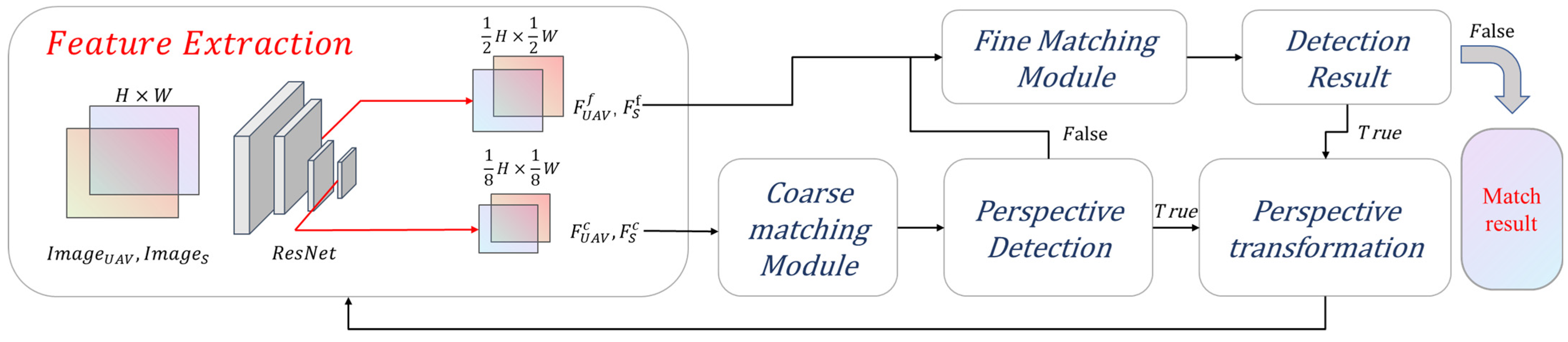
• A fast end-to-end feature-matching model is proposed. The model adopts the matching strategy from coarse to fine, and the minimum Euclidean distance is used to accelerate the coarse matching.
• The detector-free matching method and perspective transformation module are proposed to improve the matching robustness. In addition, a transformation criterion is added to ensure the efficiency of the algorithm.
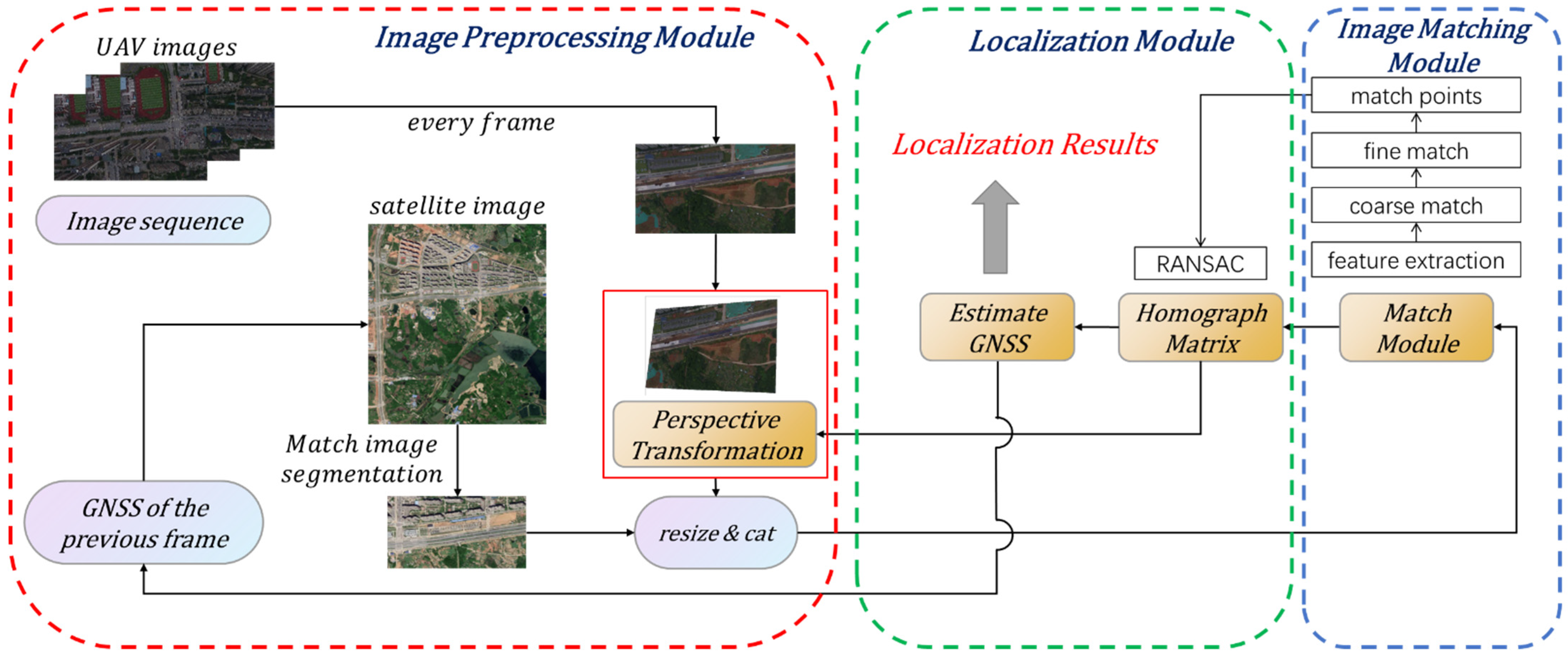
• A complete visual geo-localization system is designed, including the image preprocessing module, the image matching module, and the localization module.

The remainder of this article is organized as follows. Section 2 describes the proposed feature-matching model, perspective transformation module, and localization system. In Section 3, the effectiveness of the proposed framework is verified using both public and self-built datasets. The discussion and conclusion are in Section 4 and Section 5, respectively

2. Materials and Methods

2.1. Overview

The framework of the visual geo-localization system is shown in Figure 1. The system determines the position of the UAV images on the satellite reference images by image matching algorithm. In addition, geo-localization is realized by using the geographic information stored in the satellite image.

The whole system can be divided into three parts: The image preprocessing module is to improve the precision and efficiency of the matching method; The image matching module is the proposed image matching method; The localization module estimates the position of UAVs through the results of image matching. Since the matching results directly affect the localization precision, the image-matching module is the key module of the whole system and the focus of our research. The following sections explain the three modules in detail.

2.2. Image Preprocessing Module

The image preprocessing module is the initial part of the whole system, which preprocesses the input UAVs and satellite images. Firstly, the viewpoints of UAVs and satellite images are always different, which will adversely affect the precision and robustness of the image-matching method. Therefore, the pre-correction of UAV images is helpful in improving the matching precision. In addition, the transformation matrix calculated in the previous frame is used to achieve perspective transformation. Secondly, the efficiency of the image-matching method is closely related to the input image size. Therefore, if the satellite images with large sizes are matched directly, the localization efficiency is unacceptable. Considering the continuity of the UAVs flight, this problem can be solved by using a local reference map. The local satellite images used for matching are segmented according to the GNSS coordinates estimated in the previous frame. Note that we consider the coordinates of the starting frame to be known. If the coordinate position of the starting frame is not known, the initialization step is required. The first UAV image will be matched to the entire satellite image, which will take some time. Finally, the UAVs and satellite images will be adjusted to the input form accepted by the model. The UAVs and satellite images are put into the same batch and resized to 640 × 480.

2.3. Image Matching Module

The image-matching module receives UAVs and satellite images from the image preprocessing module and outputs the matching point pairs by the proposed image-matching method. It is clear that the precision and efficiency of the visual geo-localization depend on the performance of the image-matching method. To improve the robustness and efficiency of the matching method, a fast detector-free two-stage matching method is proposed. We will briefly introduce the design idea of the model and detail the parameter in the corresponding sections.

Firstly, the image-matching method based on feature points and feature descriptors is the most widely used method at present [11]. This typical method uses the similarity constraints of the feature descriptor to calculate matching points, then the geometric constraints between feature corresponding points are used to eliminate mismatches. The matching effect of these methods is directly related to feature point extraction and feature description. However, in sparse texture areas, it is difficult to extract repeatable feature points and perform robust feature descriptions. Because the local features of the weak texture are indistinguishable from the neighborhood features. Therefore, the extracted feature points are not robust, leading to unstable matching. The detector-free matching methods do not extract feature points, which use the entire feature maps to estimate the possible matches for all pixels and have a good performance in sparse texture areas. Therefore, this paper designs a detector-free matching model, and the ResNet (Residual Network) [39] is the feature extraction backbone.

Secondly, the matching strategy from coarse to fine is beneficial to the matching efficiency and precision [32,35]. In the coarse matching stage, the resolution of the feature map is reduced to improve the matching efficiency. Fine matching is based on the results of coarse matching, which improves the matching precision through high-resolution feature maps. Moreover, the different viewpoints of the images will have adverse effects on matching results. So, the perspective transformation module is integrated into the matching model to improve the matching robustness of the viewpoint data.

Finally, the proposed matching framework is shown in Figure 2. It is divided into four modules, namely the feature extraction module, the coarse matching module, the fine matching module, and the perspective transformation module. ResNet will extract the feature maps of the input images first, and then the feature maps will be coarse-matched. The perspective detection results will decide whether to carry out perspective transformation. If the perspective detection result is true, it will be re-matched once after coarse matching and fine matching, respectively. In a word, the processing flow is coarse matching; feature re-extraction; coarse matching; fine matching; feature re-extraction; coarse matching; fine matching; matching results. All modules are explained in detail in the following sections.

2.3.1. Feature Extraction Backbone

A residual network is used as a feature extraction backbone, for it can extract robust features. [43,44] et al. also took ResNet as the backbone of the matching model, and the experimental results fully proved the effectiveness of ResNet in extracting features. However, most of the current visual geo-localization methods use ResNet-50 to extract feature maps, which makes it difficult to apply the matching methods in light UAVs. For the consideration of efficiency and power consumption, the lighter ResNet-18 is used to extract multi-scale features. The detailed architecture and parameters are shown in Figure 3, and the output feature maps of Block2 and Block4 are extracted to realize the matching from coarse to fine.

The input of the feature extraction module is single-channel images. Firstly, the UAVs and satellite images are grayscale normalized and put into the same batch. Then, the batch of images is passed through the initial layer with a convolution kernel size of 7 × 7 and step size of 2 to generate a feature map with 128 channels. The resolution of the feature map is 1/4 of the original image size. Next, the feature map is passed through three consecutive blocks, each with a convolution kernel size of 3 × 3. In addition, there are down-sampling modules in Block3 and Block4. The number of channels output by the three blocks is 128, 192, and 256, and the feature map resolution is 1/4, 1/16, and 1/64 of the original map size, respectively. Finally, the feature maps output by Block2 and Block4 are extracted and input into different convolutional layers to get multi-scale feature maps. The purpose of using different output convolutional layers is to fine-tune coarse matching and fine matching, respectively, which is beneficial for matching precision.

2.3.2. Coarse Matching Module

The performance of the coarse matching module has a huge impact on the result, so two different matching methods are designed in the coarse matching stage. According to the research of [34,35,36], the Transformer module can effectively improve robustness and precision. The Transformer-based matching method uses the self-attention and cross-attention mechanisms to encode the features. In addition, the cost matrix is constructed by correlating the encoded features, which is used to establish the pixel-level matching results. Specifically, the SoftMax function is used to convert the cost matrix into a probability distribution matrix. The elements in the probability distribution matrix represent the matching probability of different pixels. Finally, the matching point pairs with the highest confidence is output. The cost matrix and probability distribution matrix can be calculated as Equations (1) and (2):

$$S\left(i,j\right)=F_A{F}_B^T,$$

(1)

$$P\left(i,j\right)=softmax{\left(i,·\right)}_j·softmax{\left(·,j\right)}_i,$$

(2)

where $F_A$ and $F_B$, respectively, represent the feature map encoded by Transformer, and the cost matrix is obtained by calculating the dot product between features. Compared with the general features, the features integrated with attention have a better matching effect. However, the cost of such improvement is also large. Both in the training and inference stages, the model has high requirements for hardware, which leads to the difficulty of deployment on UAVs. How to retain the precision of the Transformer while reducing the demand for hardware is an important issue in current research.

Multiple research results have shown that the attention module of the Transformer can be replaced with simpler operators. The shift module [45] and the Fourier transform [46] maintain the precision of the original model and improve efficiency without increasing the parameters. Through multiple experimental verifications, [47] thought that the architectural design of the Transformer is conducive to precision. Based on their research results, this study explores the possibility of using a simpler similarity measure method to replace the Transformer and SoftMax function.

The core of the feature matching method based on Transformer is to use an attention module to encode features. If the attention module is replaced with a simpler operator, the features are unencoded, and the features extracted by the backbone will be directly used for matching. According to the research results of [26], the pretrained VGG [48] model on ImageNet [49] can achieve robust matching. Therefore, it is possible for the feature extraction module to learn enough knowledge through the Transformer during training. Experimental results show that the feature extracted by ResNet can achieve dense matching. The matching results retain most of the precision of the pretrained model and greatly reduce the coarse matching time.

This study tests a variety of similarity measurement algorithms and finally chooses the minimum Euclidean distance matching method, which is faster and has the largest number of matching points. Figure 4 shows the coarse matching module based on Euclidean distance. The input feature map is first flattened into a 256-dimensional vector of length L, and then the cost matrix of feature points is obtained by measuring the feature similarity according to the Euclidean distance rule. The minimum values of rows and columns in the cost matrix are selected, which are converted to coordinates by mapping. In the case of one too many, the matching point with the smallest Euclidean distance is selected. The minimum Euclidean distance method can effectively accelerate the coarse matching.

2.3.3. Fine Matching Module

After the coarse matching is established, the matching point pairs obtained by the coarse matching are refined to the original image resolution by using the fine matching module. The fine-matching module framework is shown in Figure 5. The input of the module is a high-resolution feature map and coarse matching coordinates. Firstly, all the coarse matching points are located on the high-resolution feature map, and then a local window of size 5 × 5 is constructed on one of the feature maps with the matching points as the center. Then, the feature association is implemented locally through Equations (1) and (2), and the confidence matrix of size 5 × 5 is output. After the confidence matrix is constructed, the fine-matching module uses the DSNT (Differentiable Spatial to Numerical) layer [50] to refine the coordinates. The DSNT layer is a differentiable numerical variation layer, which is consistent with the training of a convolutional neural network. DSNT layer only needs to input the confidence matrix. Through the preset adjustment matrix and cross convolution, the DSNT layer outputs the pixel coordinate fine-tuning, ranging from (−1, −1) to (1, 1). The fine matching module uses the DSNT layer to adjust the coarse matching coordinates, which can achieve sub-pixel matching precision.

2.3.4. Perspective Transformation Module

The viewpoints of UAVs and satellite images are always different, which will have a negative impact on the image-matching method. The matching method performs well for data from the same perspective, but the matching precision decreases obviously in the face of the data with changing perspective. Therefore, the perspective transformation module can improve the matching precision by pre-correcting the viewpoints of the input images.

The proposed method warps the image through the homography matrix, making the input images in the same viewpoint. Firstly, in the coarse matching stage, the homography matrix is estimated after the output of the coarse matching point pairs, and the estimated homography matrix is used to correct the input matching images (The estimation method will be introduced in Section 2.4). Then the corrected images are used for matching, and the coarse matching results of the corrected images are the input of the fine matching module. The fine-matching module will output high-precision matching results. Next, the pixel coordinates are recovered by the estimated homography matrix, and the homography matrix of fine-level is estimated through the fine-level matching point. The input image will be corrected and matched again. Finally, the matching results of the second round are output.

To ensure the efficiency of matching, a correction criterion is designed to decide whether to correct. In addition, the correction criterion is based on the characteristics of the estimated homography matrix. The homography of matching point pairs can be expressed by Equation 3, and this relation can be further decomposed into Equation (4):

$$\left[\begin{array}{c}{X}^{*}\\ Y^{*}\\ Z\end{array}\right]=\left[\begin{array}{ccc}{H}_{11}& H_{12}& H_{13}\\ H_{21}& H_{22}& H_{23}\\ H_{31}& H_{32}& 1\end{array}\right]·\left[\begin{array}{c}x\\ y\\ 1\end{array}\right],$$

(3)

$$\left[\begin{array}{c}{X}^{*}\\ Y^{*}\end{array}\right]=\left[\begin{array}{cc}{H}_{11}& H_{12}\\ H_{21}& H_{22}\end{array}\right]·\left[\begin{array}{c}x\\ y\end{array}\right]+\left[\begin{array}{c}{H}_{13}\\ H_{23}\end{array}\right],$$

(4)

where $H_{ij}$ is a homography matrix element. $Z$ represents the scale factor and $X^{*}$, $Y^{*}$ are the coordinates without scale normalization. The four parameters in the upper left corner of the homography matrix control the deformation of the images, while the other parameters are only the displacement and scale change of the images. For the displacement and scale change of the images, the current matching methods have sufficient matching robustness. Therefore, based on the upper left corner four parameters, the correction criterion is designed. The matrix is compared with the two-dimensional identity matrix, and the appropriate threshold is set. The perspective transformation module ensures the matching efficiency of the same viewpoint images and enhances the matching precision of different viewpoint images.

The two-stage matching method based on the perspective transformation module effectively improves the matching precision. However, it is worth noting that the perspective transformation module will re-extract feature maps, which will adversely affect the matching efficiency. The efficiency of feature extraction affects the overall matching efficiency. Therefore, we set the perspective transformation module in the image preprocessing module to overcome this problem.

2.3.5. Training

According to the description in Section 2.3.2, the model needs to be trained twice. The first time, the Transformer based matching method is trained to obtain a robust pretrained model. The second time fine-tuned the pretrained model. The minimum Euclidean distance is used to realize coarse matching, and the fine matching module will be re-trained to improve the model matching precision.

All models were trained on the MegaDepth [51] dataset. The dataset contains multi-view images with corresponding camera parameters and depth values. However, this dataset lacks matching truth values, which are generated by the following strategy in this paper. The data is processed in four steps before training. First, two images from different perspectives of the same target are taken out, and the pixel coordinates of one image is back-projected to 3D coordinates using camera parameters and depth values. Then the camera parameters of the other image are used to project the 3D coordinates to the 2D coordinates to establish the pixel correspondence between the two images. Thirdly, in the case of occlusion or projection coordinates mismatch, the depth comparison of projection coordinates is carried out. If the difference between the estimated depth and the real depth is within a certain range, the matching truth value is determined. Finally, the confidence matrix is arranged according to the structure of the network output.

There are three reasons to use the MegaDepth dataset for training. Firstly, the MegaDepth dataset has many images and can train a more robust pretrained model. Secondly, the number of UAVs and satellite image-matching datasets is less. In addition, there is no corresponding truth supervision, so it is difficult to train the point-to-point matching model. Finally, with the increase in model depth, the feature description of the deep learning model gradually manifests as image semantics. At the same time, there is a certain similarity between UAVs and satellite images so that most matching scenes can be satisfied through semantic features. The migration of the pretrained model is feasible.

Two loss functions are used in network training. Focal loss is used in the coarse matching stage. Focal loss can alleviate the problem of loss shock. At the same time, it can set training preferences through weight allocation, which enables training to pay more attention to difficult samples. The focal loss was expressed as Equation (5):

$$L_C=-\frac{1}{\left|P_C^{gt}\right|}{\sum }_{\left(i,j\in P_C^{gt}\right)}log{P}_C\left(i,j\right),$$

(5)

where $P_C^{gt}$ represents the confidence truth value in the coarse matching stage. $P_C\left(i,j\right)$ (Equation (1)) is the probability distribution matrix inferred by a coarse matching module. $i$ and $j$, respectively, represent the pixel coordinates on two images.

The L2-norm loss is used in the fine-matching stage. During matching, the matching point pixel position of one image remains unchanged. In addition, only the pixel position of the corresponding matching point is adjusted. Therefore, the loss is calculated according to the pixel position of one image. The loss results are the coordinate error, and the calculation method is shown in Equation (6):

$$L_F=-\frac{1}{\left|P_F\right|}{\sum }_{\left(i,j\in P_F\right)}\Vert j-j_{gt}\Vert ,$$

(6)

where $i$ represents the pixel position of the reference image, $j$ represents the pixel position of the coordinate fine-tuning image. $j_{gt}$ is the ground truth calculated by camera parameters, depth, and pixel position $i$ of the reference image.

The final output loss is a sum of two parts. In addition, in the second training of the model, there is no coarse matching loss. The output loss is only the L2-norm loss.

2.4. Localization Module

The localization module receives the results of the image matching module, which is the matching point pairs between the UAVs and satellite images. The function of the localization module is to estimate the coordinate transformation matrix between UAVs and satellite images through matching point pairs. In addition, based on the geographical information stored in satellite images, the conversion between pixel coordinates of UAV images and geographical coordinates is established.

The matching point pairs can be correlated through a homography matrix. The homography matrix is usually used to describe the mapping between two images. The homography of point pairs can be expressed by Equations (3) and (7):

$$\{\begin{array}{c}X=\frac{X^{*}}{Z}=\frac{H_{11}x+H_{12}y+H_{13}}{H_{31}x+H_{32}y+1}\\ Y=\frac{Y^{*}}{Z}=\frac{H_{21}x+H_{22}y+H_{23}}{H_{31}x+H_{32}y+1}\end{array}$$

(7)

where $H_{ij}$ is a homography matrix element. $Z$ represents the scale factor and $X^{*}$, $Y^{*}$ are the coordinates without scale normalization. The normalized $X$ and $Y$ represent the pixel coordinates of UAVs images. $x$ and $y$ is the pixel coordinate of satellite images. Therefore, according to Equations (3) and (7), the homography matrix can be estimated through four pairs of matching points. However, the number of matching points exceeded four pairs. At the same time, the precision of the selected matching points will also affect the precision of the estimated homography matrix. The RANSAC (Random Sample Consensus) [52] algorithm is often used to solve the above problems. The RANSAC obtains the best homography matrix through iterative estimation.

After the homography matrix is obtained, any pixel on the UAVs images can estimate its corresponding coordinates on the satellite images. This means that the geographic information stored in satellite images can be used to achieve geo-localization. The geographic information stored in satellite images is generally expressed as six affine coefficients. Equation (8) shows the conversion of pixel coordinates to longitude and latitude.

$$\{\begin{array}{c}logitude=re{s}_{x}x+ro{t}_{y}y+A\hfill \\ latitude=ro{t}_{x}x+re{s}_{y}y+B\hfill \end{array}$$

(8)

where $re{s}_x$ and $re{s}_y$ represent the pixel resolution in the x and y directions, $ro{t}_x$ and $ro{t}_y$ represent the rotation coefficients in the x and y directions, and $A$ and $B$ represent the longitude and latitude of the pixel in the upper left corner of the satellite images.

So far, the localization module has realized the localization of a single UAV image. At the same time, the estimated homography matrix and localization results are sent back to the image preprocessing module for the UAV image pre-correction and satellite image segmentation.

3. Results

3.1. Datasets

The performance of the method is tested on the image-matching dataset HPatches [53], and the effectiveness of the proposed module is also verified. HPatches is a public dataset for image matching algorithms, which contains two parts with significant changes in illumination and large changes in viewpoint. The graphic content covers buildings, objects, creatures, landscapes, and more. The matching effect is assessed by the homography matrix.

At present, there is no public dataset for the test of visual geo-localization methods. This study constructs a test dataset. Firstly, a visual geo-localization dataset is constructed by using the public UAVs images dataset, which is from the ICRA contest (General Place Recognition: Visual Terrain Relative Navigation). Based on the UAV images provided by the contest, the satellite images of the corresponding region are captured on Google Earth. The objective index of evaluation is the satellite navigation data in the dataset. Secondly, DJI Phantom 4 RTK is used to collect orthoimages of about 6 square kilometers in the suburbs of Wuhan. The flying height of the UAV is kept at 300 m, and the resolution of the collected image is 1920 × 1080. At the same time, the satellite navigation data taken by the UAV is recorded as the basis for judging the precision of localization. The satellite base image is also captured on Google Earth. The localization precision is evaluated by analyzing the difference between algorithmic positioning and satellite positioning.

3.2. Matching Performance Experiment

The HPatches dataset is used to compare and test the performance of the algorithms. At the same time, the effectiveness of the module is verified by the ablation experiment. Each sequence in the HPatches dataset contains six images with different illumination or viewpoints. For each sequence, one image is taken as the reference image and matched with the other five images. The matching points accuracy of the algorithm is evaluated according to the homography matrix of the dataset. The precision is calculated as Equations (9)–(11):

$$Er{r}_{A2B}=L2\left(p_i^A\left(H_{pd}-H_{gt}\right)\right),$$

(9)

$$Er{r}_{B2A}=L2\left(p_i^B\left(H_{pd}^{-1}-H_{gt}^{-1}\right)\right),$$

(10)

$$precision(\%)=\frac{{\sum }_{i=0}^N[\frac{Er{r}_{A2B}+Er{r}_{B2A}}{2}<Thr]}{N},$$

(11)

where $H_{pd}$ and $H_{gt}$ represent the estimated and true values of the homography matrix, respectively. $Thr$ is pixel error.

3.2.1. Matching Point Precision

The experiment counted the matching pix error from 1 to 10. In addition, the current typical image matching methods are compared, including the detector-based matching method SIFT [17], the detector-based matching method SuperGlue (SuperPoint [14] to extract feature points, SuperGlue [34] to match. Hereinafter referred to as the SuperGlue method), the detector-free matching method LoFTR [35] and Patch2Pix [54]. The comparison methods are represented in the same types, and they are used to verify the effectiveness of the proposed method.

The precision result of matching point pairs is shown in Figure 6. In the figure, the horizontal axis represents the error of matching points relative to the true value, which ranges from 1 to 10 pixels. The vertical axis represents the proportion of matching points whose error is within the threshold. From the curve results of the graph, the matching point precision of the proposed method is ahead of the current typical matching methods. The proposed method is slightly inferior to the LoFTR method on illumination variation data. In addition, it should be noted that the precision in 4–10 pixels of the SuperGlue method is higher than that of the proposed algorithm, which is caused by the different matching frameworks. The proposed method is detector-free, which may lead to mismatched points. By contrast, the SuperGlue method is based on SuperPoint feature points. This method only matches the regions with better texture, which reduces false matching. However, as described in Section 2.3, the detector-based matching methods can’t extract repeatable features in sparse texture areas, and the robustness is not enough.

3.2.2. Homography Matrix Precision

It is not always possible to estimate the exact geometric relationship from the exact matches because the distribution and number of matches are also very important in the estimation of the homography matrix. Therefore, the homography matrix precision evaluation is carried out on HPatches. The mapping precision of the four corner points of the image is calculated, and the proportion of the estimated homography matrix with the average corner error below 1, 3, and 5 pixels is reported. The homography matrix estimation method is based on the RANSAC algorithm, and the threshold is set to 10.

The corner error of the homography matrix estimated by all algorithms is shown in

Table 1. The precision of the estimated homograph matrix. Bold indicates optimal precision.

Method	1 px	3 px	5 px
LoFTR	65.9	80.9	86.3
SuperGlue	51.3	83.6	89.1
Patch2Pix	51.0	79.2	86.4
SIFT	35.9	61.5	71.0
Proposed	66.5	84.5	90.1

. The precision of the proposed algorithm is superior to the current matching methods. The homography matrix precision is closely related to the localiazation precision. The proposed method has a more accurate homography matrix and will have better performance in the visual geo-localization system.

3.2.3. Ablation Experiment

The ablation experiment is used to demonstrate the performance of the proposed perspective transformation and minimum Euclidean distance matching module. The ablation experiment results of the perspective transformation module are shown in Figure 7. It should be noted that since the module has no effect on the illumination data, all the results of the ablation experiment are on the viewpoint dataset.

It can be clearly found from the figure that the perspective transformation module effectively improves the precision of matching points. A single perspective transformation module has greatly improved the performance of the method. The precision of matching points for viewpoints data is improved by 13%, and the number of matching points is increased by 1500 on average. Due to the improvement of matching point accuracy, homography matrix estimation has better results. As shown in

Table 2. The precision of the estimated homograph matrix with different matching strategies.

Method	1 px	3 px	5 px
direct matching	26.8	56.6	67.7
correct once	42.5	69.8	77.0
correct twice	50.3	77.3	84.4

, the homography matrix precision with different errors is improved by 13% on average. Moreover, there is still improvement after applying the perspective transformation module twice, especially for the estimated homography matrix; the precision is improved by nearly 8%. The perspective transformation module significantly improves the algorithm, which is mainly caused by two aspects: Firstly, because the Euclidean distance is a nonlinear similarity measure method, the proposed method performs poorly on the viewpoints data, and the precision is a bit low. Secondly, the matching performance of the original model is very good for the illumination data. So, the perspective transformation module can effectively utilize the advantages of the proposed method and improve the matching precision.

As for the rationality of accelerating the Transformer with minimum Euclidean distance, the common similarity measurement methods are used to replace the coarse matching module based on Transformer. The experimental results are shown in

Table 3. Statistical results of matching points with different methods.

Method	Same Points	Correct Points	Precision	Time (CPU)
Euclidean Distance	73.8(1486/2015)	95.1(503/529)	91.6(1845/2015)	0.13 s
Pearson Correlation Coefficient	74.3(1485/1997)	94.5(484/512)	92.1(1840/1997)	2.1 s
Cosine Distance	74.3(1483/1994)	95.1(486/511)	92.1(1839/1994)	0.11 s
Transformer			99.9(2157/2159)	1.3 s

.

The first column of the table is the test method, including Euclidean distance, Pearson correlation coefficient, and cosine distance. The second column shows the same points percentage of coarse matching results obtained compared with the Transformer. It can be found that the three matching methods retain more than 70% of the matching points of the original. The precision of the new match points is also about 95%, which is the result in the third column of the table. Since the coarse matching result is based on the feature map with lower resolution, the matching points with pixel error within four are considered to get the correct result through the fine matching module. The results in the table are based on the true homography matrix to count the number of matching points with pixel error within 4. From the precision of matching points, it can be found that measuring feature similarity directly can retain most of the accuracy of the original model. The last column of inference time on CPU shows that the use of a suitable similarity measure can accelerate the coarse matching speed, and both Euclidean distance and cosine distance can accelerate the coarse matching module by more than ten times. Based on the experimental results, Euclidean distance is used in the coarse matching module. Because the Euclidean distance metric obtains the most matching points and produces more high-precision matching points different from Transformer. The matching precision of the three methods is close, and the matching efficiency of Euclidean distance and cosine distance is also close. In the conventional scene, the matching performance difference between the three is not obvious. However, in the sparse texture area, the number of matching points has a great impact on the precision of the estimated homography matrix. The Euclidean distance will perform better.

3.3. Localization Precision

Localization precision is evaluated on self-built datasets. Firstly, the UAVs and local satellite images are matched, and the homography matrix is calculated according to the matching point pairs. The homography matrix is estimated using the RANSAC algorithm, and the threshold is set to 10. The coordinates of the UAVs images centered on the satellite reference map are calculated by homography matrix, and then the longitude and latitude coordinates of the UAVs are obtained by the geographic coordinates stored in the satellite map (the localization method has been introduced in Section 2.4). Because the result of SIFT method is not good, the four best matching methods are compared.

The experimental results on the ICRA dataset are shown in Figure 8. From the overall results, it can be intuitively found that the matching performance of LoFTR is not very good, and the localization is lost many times because of the bad matching results. Figure 9 shows the matching results of the four methods for the same region. The data in this region has a bit of perspective change. It can be seen from the figure that the robustness of the LoFTR method is not strong, and the number of feature points extracted is relatively small. Therefore, although the LoFTR method has achieved good results on the previous image-matching dataset, the localization effect is not good. The other three methods all get more matching points, which is conducive to localization. The proposed method gets the most matching points due to the perspective transformation module, which effectively improves the robustness of the method. Figure 8c,d shows the details of the localization trajectory. The three algorithms with better performance all have different degrees of localization fluctuations. Overall, the localization results of the proposed and SuperGlue method are relatively more stable. The Patch2Pix method has frequent fluctuations with larger amplitude.

It can also be found from the figure that the three algorithms have consistent deviation trajectories. This is because the center of the image is used as the localization center in the experiment, but the UAV localization coordinates provided by this dataset are not the center of the UAV image. As shown in Figure 10, the center of the image is different.

The localization evaluation results are shown in

Table 4. Numerical results of localization precision on ICRA dataset. The value before the slash represents the result when the number of matched images is 471. The value after the slash represents the result when the number of matched images is 601, so the LoFTR method cannot be counted. The last column indicates the number of images that are successfully matched. Bold in the second and third columns of the table indicates the minimum localization error. Bold in the last column indicates the maximum number of successfully matched images.

Method	Average Error	Max Error	Matches
LoFTR	12.01 m/×	24.61 m/×	471/601
SuperGlue	11.14 m/9.84 m	20.42 m/21.00 m	601/601
Patch2Pix	11.16 m/9.81 m	21.54 m/21.54 m	601/601
Proposed	11.13 m/9.80 m	20.14 m/20.72 m	601/601

. Overall, the precision of the three algorithms with better effects is close to each other, no matter the average error or the maximum error. It should be noted that the average error and maximum error only count the successful part, and the judgment basis is whether the positioning deviation is greater than 25 m. Therefore, the maximum error of the LoFTR method is 24.61 m. Although the true value of this dataset is biased and the result is not objective, it also reflects the performance of the algorithm to a certain extent.

To evaluate the algorithm more objectively, the experiment is repeated on the self-built dataset, and the experimental results are shown in Figure 11. From the resulting figure, it can be found that although SuperGlue achieved ideal results on the ICRA localization dataset, it lost localization in the jungle area of the self-built dataset. This is caused by the inherent defects of detector-based matching methods, which are usually unable to obtain robust feature points in sparse texture areas, so it is difficult to establish stable matching. The LoFTR algorithm also lost its location in the jungle area. Patch2Pix does not lose localization compared with other algorithms, but like the results on the ICRA localization dataset, the localization fluctuation ratio is larger than the other method. Positioning is closely related to the flight stability of UAVs. Unstable positioning will have adverse effects on the flight control of UAVs. The stability of the Patch2Pix algorithm is not sufficient. The results show that the stability and robustness of the proposed model are good.

Figure 12 shows the matching results of different methods in texture sparse regions. From the matching results, it can be clearly found that the proposed method with the perspective module outputs the most matching points with obvious advantages. In weak texture regions, the number of repeatable matching points is the basis for good estimation, so the proposed algorithm can achieve high-precision matching localization in sparse texture regions. Although the matching points of Patch2Pix are few, the precision of matching points is enough for localization. However, the localization precision is affected, leading to great localization fluctuations. In addition, the proposed method without a single perspective transformation module has the same results. The SuperGlue and LoFTR methods deviate from the location due to the insufficient accuracy of matching points. Through the qualitative analysis of the matching results. In sparse texture areas, the number and precision of matching points affect the accuracy of localization, so the proposed method achieves the best localization results. Secondly, the proposed perspective transformation module is beneficial to improve the robustness of the algorithm in weak textures.

The GNSS coordinates are also used for objective evaluation, and the statistical results are shown in

Table 5. Numerical results of localization precision on the self-build dataset. The value before the slash represents the result when the number of matched images is 423. The value after the slash represents the result when the number of matched images is 792, so the LoFTR and SuperGlue method cannot be counted. The last column indicates the number of images that are successfully matched. Bold in the second and third columns of the table indicates the minimum localization error. Bold in the last column indicates the maximum number of successfully matched images.

Method	Average Error	Max Error	Matches
LoFTR	3.31 m/×	8.80 m/×	432/792
SuperGlue	3.21 m/×	8.50 m/×	423/792
Patch2Pix	3.30 m/2.57 m	8.60 m/14.48 m	792/792
Proposed	3.17 m/2.24 m	8.60 m/14.16 m	792/792

. From the results in the table, it can be found that the performance of the algorithm is different in areas with sparse texture. In the rich textured area, that is, the data before the slash in the table. The SuperGlue method has high precision, and the maximum error is optimal. The average error of the proposed algorithm is optimal. The proposed method is more stable and has better localization precision. In the sparse texture area, the SuperGlue method cannot output stable matching due to the inherent defects of the algorithm. Although the matching precision of Patch2Pix and the proposed method is greatly affected, they achieve stable matching. However, the results of the Patch2Pix method fluctuate greatly, so the average error and maximum error of the proposed method are greatly improved compared with it. According to the subjective and objective evaluation, the proposed method achieves the best localization precision and completes matching and localizing the entire dataset, which proves the advancement of the proposed method.

3.4. Efficiency

Since the calculation power of UAVs is limited, the algorithm efficiency must be considered. The efficiency of different methods is compared on Jetson Xavier NX, and the results are shown in

Table 6. Matching the speed of different methods on Jetson Xavier NX. The three times of the proposed method in the table correspond to direct matching, the model with single and double perspective transformation modules, respectively.

Method	Time
LoFTR	1.84 s
SuperGlue	0.80 s
Patch2Pix	2.20 s
Proposed	0.65 s/1.03 s/1.46 s

. The direct matching method has the highest efficiency compared with other methods when precision is ensured. Although the perspective transformation module affects the matching efficiency, the proposed method still has greater efficiency than LoFTR and Patch2Pix. The SuperGlue method has good efficiency, but the matching efficiency of the SuperGlue model is closely related to the number of feature points. The number of feature points in the matching time of 0.8 s is 300. When the number of matching points increases to about 400, the time also increases to 0.83 s. In addition, the SuperGlue method cannot match images stably in weak texture areas, which leads to localization loss.

4. Discussion

The experimental results showed that the proposed method improves the localization precision by 12.84% and the localization efficiency by 18.75% compared with the current typical methods. The superior performance of the method can be attributed to several aspects.

Considering the computing power limitation of the UAVs, we choose resnet18 as the feature extraction backbone. In the coarse matching stage, the matching is accelerated by reducing the resolution and the minimum Euclidean distance. The ablation experiment on Hpatches shows that the minimum Euclidean distance retains 91.6% precision of the pretrained model, which greatly improves the matching efficiency at the same time. In addition, the efficiency of different methods is compared on Jetson Xavier NX. The single matching time of the proposed method is 0.65 s, which is superior to the current typical methods. In the fine-matching stage, the coordinates are refined by using high-resolution feature maps. We adopt the DSNT layer in the fine matching module, which is a differentiable numerical variation layer that can achieve sub-pixel matching precision. The experimental results on the Hpatches dataset show that our method has a precision advantage in both matching points and homography estimation.

Moreover, the experimental results showed that the method is superior in the scene of the weak texture and viewpoint change. Availability to weak texture data is attributed to the detector-free method, which estimates possible matches for all pixels to attain more stable matching points, and the transformer is used to generate a pretrained model which integrates local and global features of the image to obtain stronger feature expression. We tested the matching methods on the self-built dataset, and the results show that the proposed method achieves the most robust matching. The proposed method outputs the most matching points in the weak texture region. Moreover, our method achieves the optimal localization precision of 2.24 m. The perspective transformation module is used as image rectification to enhance the adaptability of the model to the viewpoint data. The ablation experiment on the Hpatches dataset demonstrates its effectiveness. The precision of matching points for viewpoints data is improved by 15%, while the number of matching points is increased by 1500 on average. In addition, the estimated homography matrix precision is improved by 21%. The subsequent experimental results on the ICRA dataset also show that the proposed method is robust to viewpoint changes.

However, the proposed method still needs to be improved in two aspects. According to the efficiency experimental results, the matching time of 0.65 s is still insufficient for application in real-time systems. Moreover, the results of localization experiments show that the trajectory of visual geo-localization is not smooth. Because the localization of different frames is independent of each other and the errors of the matching method are unstable. The correlation of consecutive frames should be utilized.

5. Conclusions

This paper proposed a faster and more robust image-matching method for UAVs visual geo-localization. A detector-free two-stage matching method with resnet18 and transformer is more available to weak texture data. A perspective transformation module improves the robustness of the viewpoint data. The minimum Euclidean distance matching is used to speed up the inference. The DSNT layer achieves sub-pixel matching precision. Moreover, a complete visual geo-localization system is designed and verified on self-built datasets. The proposed method obtains excellent results in both subjective and objective evaluation. Finally, the efficiency experiment on Jetson Xavier NX shows that the proposed method can achieve fast and robust localization for UAVs.

Although the proposed model has proven to be precise, robust, and efficient, additional time cost by the perspective transformation module by re-extracting the corrected image features is not satisfactory enough, in particular, for the reuse of the module. In addition, the lack of the correlation of consecutive frames maybe caused the positioning trajectory to be not smooth. The above two problems need to be improved during the next work.

References

1. Kazerouni, I.A.; Fitzgerald, L.; Dooly, G.; Toal, D. A Survey of State-of-the-Art on Visual SLAM. Expert Syst. Appl. 2022, 205, 117734. [Google Scholar] [CrossRef]
2. Gyagenda, N.; Hatilima, J.V.; Roth, H.; Zhmud, V. A review of GNSS-independent UAV navigation techniques. Robot. Auton. Syst. 2022, 152, 104069. [Google Scholar] [CrossRef]
3. Couturier, A.; Akhloufi, M.A. A review on absolute visual localization for UAV. Robot. Auton. Syst. 2021, 135, 103666. [Google Scholar] [CrossRef]
4. Alkendi, Y.; Seneviratne, L.; Zweiri, Y. State of the art in vision-based localization techniques for autonomous navigation systems. IEEE Access 2021, 9, 76847–76874. [Google Scholar] [CrossRef]
5. Hu, K.; Wu, J.; Zheng, F.; Zhang, Y.; Chen, X. A survey of visual odometry. Nanjing Xinxi Gongcheng Daxue Xuebao 2021, 13, 269–280. [Google Scholar]
6. Jin, Z.; Wang, X.; Moran, B.; Pan, Q.; Zhao, C. Multi-region scene matching based localisation for autonomous vision navigation of UAVs. J. Navig. 2016, 69, 1215–1233. [Google Scholar] [CrossRef]
7. Yu, Q.; Shang, Y.; Liu, X.; Lei, Z.; Li, X.; Zhu, X.; Liu, X.; Yang, X.; Su, A.; Zhang, X.; et al. Full-parameter vision navigation based on scene matching for aircrafts. Sci. China Inf. Sci. 2014, 57, 1–10. [Google Scholar] [CrossRef] [Green Version]
8. Kaur, R.; Devendran, V. Image Matching Techniques: A Review. Inf. Commun. Technol. Compet. Strateg. 2021, 401, 785–795. [Google Scholar]
9. Chen, L.; Heipke, C. Deep learning feature representation for image matching under large viewpoint and viewing direction change. ISPRS J. Photogramm. Remote Sens. 2022, 190, 94–112. [Google Scholar] [CrossRef]
10. Jiang, X.; Ma, J.; Xiao, G.; Shao, Z.; Guo, X. A review of multimodal image matching: Methods and applications. Inf. Fusion 2021, 73, 22–71. [Google Scholar] [CrossRef]
11. Ma, J.; Jiang, X.; Fan, A.; Jiang, J.; Yan, J. Image matching from handcrafted to deep features: A survey. Int. J. Comput. Vis. 2021, 129, 23–79. [Google Scholar] [CrossRef]
12. Yao, G.; Yilmaz, A.; Meng, F.; Zhang, L. Review of Wide-Baseline Stereo Image Matching Based on Deep Learning. Remote Sens. 2021, 13, 3247. [Google Scholar] [CrossRef]
13. Harris, C.; Stephens, M. A combined corner and edge detector. In Alvey Vision Conference; dblp: Saarland, Germany, 1988; Volume 15, pp. 10–5244. Available online: https://dblp.org/db/conf/bmvc/index.html (accessed on 3 October 2022).
14. Trajković, M.; Hedley, M. Fast corner detection. Image Vis. Comput. 1998, 16, 75–87. [Google Scholar] [CrossRef]
15. Rublee, E.; Rabaud, V.; Konolige, K.; Bradski, G. ORB: An efficient alternative to SIFT or SURF. In Proceedings of the International Conference on Computer Vision, Barcelona, Spain, 6–13 November 2011; pp. 2564–2571. [Google Scholar]
16. Calonder, M.; Lepetit, V.; Strecha, C.; Fua, P. Brief: Binary robust independent elementary features. In European Conference on Computer Vision; Springer: Berlin/Heidelberg, Germany, 2010; pp. 778–792. [Google Scholar]
17. LOWE, D.G. Distinctive image features from scale-invariant keypoints. Int. J. Comput. Vis. 2004, 60, 91–110. [Google Scholar] [CrossRef]
18. Bay, H.; Tuytelaars, T.; Gool, L.V. Surf: Speeded up robust features. In European Conference on Computer Vision; Springer: Berlin/Heidelberg, Germany, 2006; Volume 3951, pp. 404–417. [Google Scholar]
19. Matas, J.; Chum, O.; Urban, M.; Pajdla, T. Robust wide-baseline stereo from maximally stable extremal regions. Image Vis. Comput. 2004, 22, 761–767. [Google Scholar] [CrossRef]
20. Yi, K.M.; Trulls, E.; Lepetit, V.; Fua, P. Lift: Learned invariant feature transform. In European Conference on Computer Vision; Springer: Cham, Switzerland, 2016; Volume 9910, pp. 467–483. [Google Scholar]
21. Zhang, X.; Yu, F.; Karaman, S.; Chang, S. Learning discriminative and transformation covariant local feature detectors. In Proceedings of the IEEE Conference on Computer Vision and Pattern Recognition (CVPR); IEEE Xplore: Washington, DC, USA, 2017; pp. 6818–6826. [Google Scholar]
22. DeTone, D.; Malisiewicz, T.; Rabinovich, A. Superpoint: Self-supervised interest point detection and description. In Proceedings of the IEEE/CVF Conference on Computer Vision and Pattern Recognition (CVPR); IEEE Xplore: Washington, DC, USA, 2017; pp. 224–236. [Google Scholar]
23. Ono, Y.; Trulls, E.; Fua, P.; Yi, K.M. LF-Net: Learning local features from images. In Advances in Neural Information Processing Systems; MIT Press: Cambridge, MA, USA, 2018; Volume 31. [Google Scholar]
24. Dusmanu, M.; Rocco, I.; Pajdla, T.; Pollefeys, M.; Sivic, J.; Torii, A.; Sattler, T. D2-net: A trainable cnn for joint description and detection of local features. In Proceedings of the IEEE/CVF Conference on Computer Vision and Pattern Recognition (CVPR); IEEE Xplore: Washington, DC, USA, 2019; pp. 8092–8101. [Google Scholar]
25. Chen, H.; Luo, Z.; Zhang, J.; Zhou, L.; Bai, X.; Hu, Z.; Tai, C.; Quan, L. Learning to match features with seeded graph matching network. In Proceedings of the IEEE/CVF Conference on Computer Vision and Pattern Recognition (CVPR); IEEE Xplore: Washington, DC, USA, 2021; pp. 6301–6310. [Google Scholar]
26. Efe, U.; Ince, K.G.; Alatan, A. Dfm: A performance baseline for deep feature matching. In Proceedings of the IEEE/CVF Conference on Computer Vision and Pattern Recognition; IEEE Xplore: Washington, DC, USA, 2021; pp. 4284–4293. [Google Scholar]
27. Revaud, J.; Leroy, V.; Weinzaepfel, P.; Chidlovskii, B. PUMP: Pyramidal and Uniqueness Matching Priors for Unsupervised Learning of Local Descriptors. In Proceedings of the IEEE/CVF Conference on Computer Vision and Pattern Recognition (CVPR); IEEE Xplore: Washington, DC, USA, 2022; pp. 3926–3936. [Google Scholar]
28. Liu, C.; Yuen, J.; Torralba, A. Sift flow: Dense correspondence across scenes and its applications. IEEE Trans. Pattern Anal. Mach. Intell. 2010, 33, 978–994. [Google Scholar] [CrossRef] [Green Version]
29. Choy, C.B.; Gwak, J.; Savarese, S.; Chandraker, M. Universal correspondence network. In Advances in Neural Information Processing Systems; MIT Press: Cambridge, MA, USA, 2016; Volume 29. [Google Scholar]
30. Schmidt, T.; Newcombe, R.; Fox, D. Self-supervised visual descriptor learning for dense correspon-dence. IEEE Robot. Autom. Lett. 2016, 2, 420–427. [Google Scholar] [CrossRef]
31. Rocco, I.; Cimpoi, M.; Arandjelovi, R.; Torii, A.; Pajdla, T.; Sivic, J. Ncnet: Neighbourhood consensus networks for estimating image correspondences. IEEE Trans. Pattern Anal. Mach. Intell. 2020, 44, 1020–1034. [Google Scholar] [CrossRef]
32. Liu, J.; Zhang, X. DRC-NET: Densely Connected Recurrent Convolutional Neural Network for Speech Dereverberation. In Proceedings of the ICASSP 2022–2022 IEEE International Conference on Acoustics, Speech and Signal Processing (ICASSP), Singapore, 23–27 May 2022; pp. 166–170. [Google Scholar]
33. Vaswani, A.; Shazeer, N.; Parmar, N.; Uszkoreit, J.; Jones, L.; Gomez, A.N.; Kaiser, L.; Polosukhin, I. Attention is all you need. In Advances in Neural Information Processing Systems; MIT Press: Cambridge, MA, USA, 2017; Volume 30. [Google Scholar]
34. Sarlin, P.E.; DeTone, D.; Malisiewicz, T.; Rabinovich, A. Superglue: Learning feature matching with graph neural networks. In Proceedings of the IEEE/CVF Conference on Computer Vision and Pattern Recognition (CVPR); IEEE Xplore: Washington, DC, USA, 2020; pp. 4938–4947. [Google Scholar]
35. Sun, J.; Shen, Z.; Wang, Y.; Bao, H.; Zhou, X. LoFTR: Detector-free local feature matching with transformers. In Proceedings of the IEEE/CVF Conference on Computer Vision and Pattern Recognition (CVPR); IEEE Xplore: Washington, DC, USA, 2021; pp. 8922–8931. [Google Scholar]
36. Wang, Q.; Zhang, J.; Yang, K.; Peng, K.; Stiefelhagen, R. MatchFormer: Interleaving Attention in Transformers for Feature Matching; Karlsruhe Institute of Technology: Karlsruhe, Germany, 2022; to be submitted. [Google Scholar]
37. Liu, Y.; Tao, J.; Kong, D.; Zhang, Y.; Li, P. A Visual Compass Based on Point and Line Features for UA V High-Altitude Orientation Estimation. Remote Sens. 2022, 14, 1430. [Google Scholar] [CrossRef]
38. Zhang, Y.; Ma, G.; Wu, J. Air-Ground Multi-Source Image Matching Based on High-Precision Reference Image. Remote Sens. 2022, 14, 588. [Google Scholar] [CrossRef]
39. He, K.; Zhang, X.; Ren, S.; Sun, J. Deep residual learning for image recognition. In Proceedings of the IEEE/CVF Conference on Computer Vision and Pattern Recognition (CVPR); IEEE Xplore: Washington, DC, USA, 2016; pp. 770–778. [Google Scholar]
40. Wen, K.; Chu, J.; Chen, J.; Chen, Y.; Cai, J. MO SiamRPN with Weight Adaptive Joint MIoU for UAV Visual Localization. Remote Sens. 2022, 14, 4467. [Google Scholar] [CrossRef]
41. Wang, T.; Zheng, Z.; Yan, C.; Zhang, J.; Sun, Y.; Zheng, B.; Yang, Y. Each part matters: Local patterns facilitate cross-view geo-localization. IEEE Trans. Circuits Syst. Video Technol. 2021, 32, 867–879. [Google Scholar] [CrossRef]
42. Zheng, Z.; Wei, Y.; Yang, Y. University-1652: A multi-view multi-source benchmark for drone-based geo-localization. In Proceedings of the 28th ACM International Conference on Multimedia; Association for Computing Machinery: New York, NY, USA, 2020; pp. 1395–1403. [Google Scholar]
43. Ding, L.; Zhou, J.; Meng, L.; Long, Z. A practical cross-view image matching method between UAV and satellite for UAV-based geo-localization. Remote Sens. 2020, 13, 47. [Google Scholar] [CrossRef]
44. Zhuang, J.; Dai, M.; Chen, X.; Zheng, E. A Faster and More Effective Cross-View Matching Method of UAV and Satellite Images for UAV Geolocalization. Remote Sens. 2021, 13, 3979. [Google Scholar] [CrossRef]
45. Wang, G.; Zhao, Y.; Tang, C.; Luo, C.; Zeng, W. When Shift Operation Meets Vision Transformer: An Extremely Simple Alternative to Attention Mechanism; University of Science and Technology of China: Hefei, China, 2022; to be submitted. [Google Scholar]
46. Lee-Thorp, J.; Ainslie, J.; Eckstein, I.; Ontanon, S. FNet: Mixing tokens with fourier transforms. In Proceedings of the North American Chapter of the Association for Computational Linguistics: Human Language Technologies (NAACL), Seattle, WA, USA, 10–15 July 2022. [Google Scholar]
47. Yu, W.; Luo, M.; Zhou, P.; Si, C.; Zhou, Y.; Wang, X.; Feng, J.; Yan, S. Metaformer is actually what you need for vision. In Proceedings of the IEEE/CVF Conference on Computer Vision and Pattern Recognition; IEEE Xplore: Washington, DC, USA, 2022; pp. 10819–10829. [Google Scholar]
48. Simonyan, K.; Zisserman, A. Very deep convolutional networks for large-scale image recognition. In Proceedings of the International Conference on Learning Representations (ICLR), San Diego, CA, USA, 7–9 May 2015. [Google Scholar]
49. Krizhevsky, A.; Sutskever, I.; Hinton, G.E. Imagenet classification with deep convolutional neural networks. Commun. ACM 2017, 60, 84–90. [Google Scholar] [CrossRef] [Green Version]
50. Nibali, A.; He, Z.; Morgan, S.; Prendergast, L. Numerical Coordinate Regression with Convolutional Neural Networks; La Trobe University: Melbourne, Australia, 2018; to be submitted. [Google Scholar]
51. Li, Z.; Snavely, N. Megadepth: Learning single-view depth prediction from internet photos. In Proceedings of the IEEE/CVF Conference on Computer Vision and Pattern Recognition (CVPR); IEEE Xplore: Washington, DC, USA, 2018; pp. 2041–2050. [Google Scholar]
52. Fischler, M.A.; Bolles, R.C. Random sample consensus: A paradigm for model fitting with applications to image analysis and automated cartography. Commun. ACM 1981, 24, 381–395. [Google Scholar] [CrossRef]
53. Balntas, V.; Lenc, K.; Vedaldi, A.; Mikolajczyk, K. HPatches: A benchmark and evaluation of handcrafted and learned local descriptors. In Proceedings of the IEEE/CVF Conference on Computer Vision and Pattern Recognition (CVPR); IEEE Xplore: Washington, DC, USA, 2017; pp. 5173–5182. [Google Scholar]
54. Zhou, Q.; Sattler, T.; Leal-Taixe, L. Patch2pix: Epipolar-guided pixel-level correspondences. In Proceedings of the IEEE/CVF Conference on Computer Vision and Pattern Recognition (CVPR); IEEE Xplore: Washington, DC, USA, 2021; pp. 4669–4678. [Google Scholar]
Figure 1. The framework of a visual geo-localization system based on image matching. The red box is the image preprocessing module, the green box is the localization module, and the blue box is the image matching module.
Remotesensing 14 05879 g001
Figure 2. The framework of the proposed image matching model.
Remotesensing 14 05879 g002
Figure 3. The framework and parameters of the feature extraction model.
Remotesensing 14 05879 g003
Figure 4. Coarse matching module.
Remotesensing 14 05879 g004
Figure 5. Fine matching module.
Remotesensing 14 05879 g005
Figure 6. Matching point precision of different methods.
Remotesensing 14 05879 g006
Figure 7. Matching point precision with different matching strategies. The gray curve with a circular marker represents the proposed method that is corrected twice in the coarse-matching and fine-matching stages, the green curve with a plus sign marker represents the method that is corrected in the coarse-matching stage, and the red curve with a triangular marker represents the matching result without perspective transformation module.
Remotesensing 14 05879 g007
Figure 8. The localized trajectory of all methods on the ICRA dataset: (a) the whole trajectory. The red line represents the GNSS reference trajectory. The green, blue, gray, and white represent the positioning trajectory of the SuperGlue method, LoFTR method, Patch2Pix method, and the proposed method, respectively; (b) local trajectory; (c) the beginning of the trajectory; (d) the end of the trajectory.
Remotesensing 14 05879 g008
Figure 9. Matching results for the same area: (a) the LoFTR method; (b) the SuperGlue method; (c) the Patch2Pix method; (d) the proposed method.
Remotesensing 14 05879 g009
Figure 10. The localization truth value provided by the dataset has deviation: (a) The blue dot on the image is the center of the UAV image; (b) The blue dot on the image is the UAVs position converted to satellite images using GNSS coordinates.
Remotesensing 14 05879 g010
Figure 11. The localized trajectory of all methods on the self-build dataset. The red line represents the GNSS reference trajectory. The green, blue, gray, and white represent the positioning trajectory of the SuperGlue algorithm, LoFTR algorithm, Patch2PIx algorithm, and the proposed algorithm, respectively. The small window in the figure shows the details of the trajectory.
Remotesensing 14 05879 g011
Figure 12. Matching results of weak texture images: (a) the LoFTR method; (b) the SuperGlue method; (c) the Patch2Pix method; (d) the proposed method without single perspective transformation module; (e) the proposed method with single perspective transformation module; (f) the proposed method with double perspective transformation modules.
Remotesensing 14 05879 g012