Abstract
Satellites are an effective source of atmospheric carbon dioxide (CO2) monitoring; however, city-scale monitoring of atmospheric CO2 through space-borne observations is still a challenging task due to the trivial change in atmospheric CO2 concentration compared to its natural variability and background concentration. In this study, we attempted to evaluate the potential of space-based observations to monitor atmospheric CO2 changes at the city scale through simple data-driven analyses. We used the column-averaged dry-air mole fraction of CO2 (XCO2) from the Carbon Observatory 2 (OCO-2) and the anthropogenic CO2 emissions provided by the Open-Data Inventory for Anthropogenic Carbon dioxide (ODIAC) product to explain the scenario of CO2 over 120 districts of Pakistan. To study the anthropogenic CO2 through space-borne observations, XCO2 anomalies (MXCO2) were estimated from OCO-2 retrievals within the spatial boundary of each district, and then the overall spatial distribution pattern of the MXCO2 was analyzed with several datasets including the ODIAC emissions, NO2 tropospheric column, fire locations, cropland, nighttime lights and population density. All the datasets showed a similarity in the spatial distribution pattern. The satellite detected higher CO2 concentrations over the cities located along the China–Pakistan Economic Corridor (CPEC) routes. The CPEC is a large-scale trading partnership between Pakistan and China and large-scale development has been carried out along the CPEC routes over the last decade. Furthermore, the cities were ranked based on mean ODIAC emissions and MXCO2 estimates. The satellite-derived estimates showed a good consistency with the ODIAC emissions at higher values; however, deviations between the two datasets were observed at lower values. To further study the relationship of MXCO2 and ODIAC emissions with each other and with some other datasets such as population density and NO2 tropospheric column, statistical analyses were carried out among the datasets. Strong and significant correlations were observed among all the datasets.
1. Introduction
Atmospheric carbon dioxide (CO2) is an important greenhouse gas (GHG) due to its significant contribution to climate change [1]. The concentration of atmospheric CO2 is continuously increasing primarily due to anthropogenic activities [2], and if it keeps on increasing at the same rate, then around 1.5 °C of global warming may be reached by the middle of this century, which may cause more climate extremes [3]. Under the Paris agreement, it has been pledged to limit global warming to well below 2 °C relative to the pre-industrial levels [4]. To meet the goals of the Paris agreement, immediate efforts are required to reduce anthropogenic emissions including CO2 emissions. Moreover, the regular monitoring of CO2 emissions using reliable datasets is also important to investigate the spatiotemporal trends of CO2 and evaluate the effectiveness of the reduction policies. However, larger uncertainties in the existing datasets and the unavailability of any reliable global system for monitoring CO2 emissions from local sources create a hindrance in monitoring CO2 at smaller scales with sufficient accuracy [5].
The atmospheric CO2 concentration is continuously increasing, and accurate measurement of changes in the concentration of atmospheric CO2 is a prerequisite to determining its influence on climate change. Several networks have been established in the world for the precise monitoring of atmospheric CO2 including the Global Atmospheric Watch (GAW) sites [6], the Collaborative Carbon Column Observing Network (COCCON) [7,8], and the Total Carbon Column Observing Network (TCCON) [9]. However, the measurements obtained from these ground stations are not sufficient for the accurate monitoring of atmospheric CO2 at regional and global scales due to certain limitations including their uneven distribution and limited spatial coverage [10]. Atmospheric CO2 monitoring has been improved with the launch of satellites because satellites can cover a very large area and provide large quantities of sampling data. The information related to atmospheric CO2 concentration has been retrieved using various sensors onboard different satellites. For instance, the concentration of atmospheric CO2 has been retrieved using the thermal infrared (TIR) bands of the Infrared Atmospheric Sounding Interferometer (IASI) [11], the Atmospheric Infrared Sounder (AIRS) [12], and Tropospheric Emission Spectrometer (TES) [13]; however, the TIR bands have lower sensitivity to the lower troposphere where most of the CO2 sources and sinks reside. The Scanning Imaging Absorption Spectrometer for Atmospheric Chartography (SCIAMACHY) employed on the European Space Agency’s (ESA) ENVISAT was the pathfinder instrument that first detected atmospheric CO2 signals using shortwave infrared (SWIR) and near-infrared (NIR) bands, which were more sensitive to lower tropospheric CO2 concentrations and provided a reliable column-averaged dry-air mole fraction of CO2 (XCO2) observations at global scales [14]. SCIAMACHY suspended its services in 2012; however, several satellites have been launched since then for the exclusive monitoring of greenhouse gases with great spatiotemporal resolutions. The Greenhouse Gases Observing Satellite (GOSAT) was the first satellite that was launched by Japan in 2009 for the monitoring of atmospheric CO2 and methane (CH4) [15]. In 2014, the National Aeronautics and Space Administration (NASA) launched a satellite, the Orbing Carbon Observatory 2 (OCO-2) that is dedicatedly monitoring the atmospheric CO2 and providing high-resolution observations. The Chinese CO2-monitoring satellite TanSat that launched in December 2016 is also capable of providing space-based CO2 measurements and preliminary XCO2 maps generated using the satellite measurements, which have been discussed in a recent study [16]. Moreover, most recently GOSAT-2 and OCO-3 have also been successfully launched for monitoring atmospheric CO2 and the initial results have been discussed in recent studies [17,18].
The global climate crisis poses several threats to Pakistan and the German Watch, an independent development and environmental non-governmental organization (NGO) that lists Pakistan among the ten countries that have been most affected by climate change during the last two decades. According to the Global Climate Risk Index (GCRI), Pakistan has suffered serious economic losses per unit GDP (Gross Domestic Product) due to 152 extreme weather events from 1999 to 2018 [19]. In a report published by the ActionAid, Bread for the World, and the Climate Action Network—South Asia (CANSA), it has been notified that even with the active emission reduction efforts, around 600,000 people will migrate by 2030 due to the impacts of climate change in Pakistan, and this number will be doubled if active actions are not carried out. The Government of Pakistan (GOP) is actively working at policy, management, and operational levels to deal with the effects of climate change. The Eco-system Restoration Initiative (ESRI) has been launched by the GOP to facilitate the transition towards an environmentally resilient Pakistan by mainstreaming adaptation and mitigation through ecological initiatives. The ESRI includes several programs including biodiversity conservation, mass-scale afforestation, and formulating environmental policies in line with the objectives of the country’s Nationally Determined Contribution (NDC) and attaining Land Degradation Neutrality (LDN). Monitoring the long-term trends of CO2 over Pakistan under the background of climate change is important for predicting future CO2 scenarios in the country.
OCO-2 was not a mapping mission, but it was designed as a sampling mission, so it samples a small portion of the globe every day [20]. OCO-2 was launched with a primary objective to monitor the atmospheric CO2 at a regional scale; however, several studies have used the OCO-2 dataset for local-scale studies due to its precise measurements [4,21,22,23,24,25]. In this study, we used the XCO2 retrievals from OCO-2 along with other datasets including the ODIAC CO2 emissions, and the Ozone Monitoring Instrument (OMI) NO2 tropospheric column to study the CO2 scenario over 120 districts of Pakistan. Moreover, the districts were also ranked based on mean anthropogenic CO2 concentrations and emissions. Additionally, spatial distribution patterns of various datasets were also compared. The description of the methods and datasets is given in Section 2; results are discussed in Section 4 and conclusions are provided in Section 5.
2. Materials and Methods
2.1. Study Area
Pakistan, with a population of around 220 million, is the fifth-most populated country in the world and is located in south Asia between 23°35′ to 37°05′ north and 60°50′ to 77°50′ east [26]. Geographically, it shares its borders with the largest CO2-emitting nations such as China, India, and Iran. Administratively, Pakistan is divided into six units: Azad Kashmir, Gilgit Baltistan, Balochistan, Khyber Pakhtunkhwa, Punjab, and Sindh. Punjab is the most populous administrative unit followed by Sindh, Khyber Pakhtunkhwa, and Balochistan. In terms of area, Balochistan is the largest administrative unit of Pakistan followed by Punjab, Sindh, and Khyber Pakhtunkhwa. The administrative units are further subdivided into districts and this study is carried out over 120 districts in Pakistan. Although Pakistan has more than 120 districts in total, some smaller districts are merged into the neighboring districts to meet the defined area requirements (>1000 km2). The area requirements were defined so that the number of satellites were sufficient. The spatial boundaries of these districts located in various administrative units are shown in Figure 1a. In addition, the topography and landcover distribution of Pakistan are shown in Figure 1b,c, respectively.
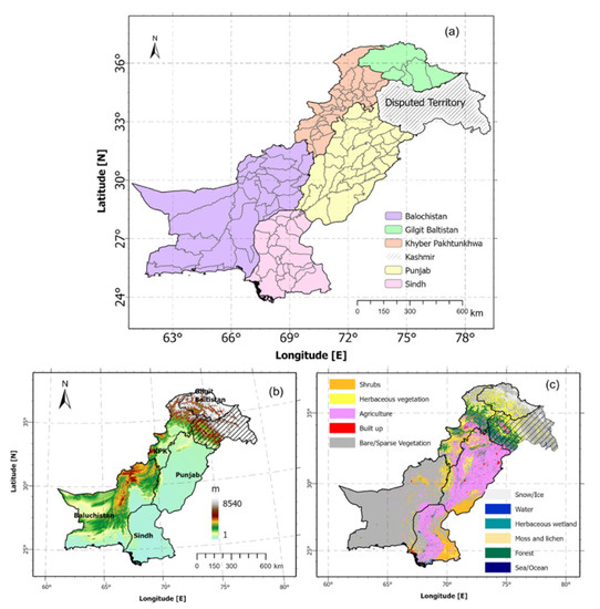
Figure 1.
(a) District and administrative unit boundaries, (b) topography and (c) landcover map of Pakistan. The shaded area shows the disputed territory of Kashmir.
2.2. Datasets
2.2.1. OCO-2 XCO2 Dataset
OCO-2 was successfully launched by NASA from the Vandenberg Air Force Base in California on 2 July 2014 for the exclusive monitoring of atmospheric CO2 at regional levels. After completing a series of check-out activities and orbit-raising maneuvers, it joined the front of the Afternoon Constellation (A-Train) on 3 August 2014 [20]. The referenced constellation consisted of six satellites orbiting around the earth at an altitude of 705 km. OCO-2 completes an orbit in 98.8 min and samples at a local time of about 1:30 pm, and it has a set of 233 orbit paths that repeat in 16-day cycles. OCO-2 has been routinely providing around 1 million soundings every day since 6 September 2014. The spatial resolution of OCO-2 at nadir is about 1.3 × 2.25 km.
The spectrometer installed on the OCO-2 satellite measures the near-infrared spectra of sunlight reflected off the Earth’s surface in three spectral regions centered at 0.765, 1.61, and 2.06 μm [27,28]. OCO-2 observations are processed using the Atmospheric CO2 Observations from Space (ACOS) Full Physics (FP) retrieval algorithm to generate a level 2 (L2) product that provides XCO2 retrievals. Technical details about the ACOS FP algorithm are given in the previous literature [29,30]. Several versions of XCO2 L2 products have been released by the OCO-2 team and have been regularly validated against accurate measurements [2,31,32,33,34]. The validation results showed that the OCO-2 datasets were consistent and reliable for atmospheric CO2 monitoring. A recent study [35] compared the latest OCO-2 XCO2 product (v10) against accurate measurements and reported a sounding precision of ~0.8 ppm over land and ~0.5 ppm over water, and RMS biases of 0.5–0.7 ppm over both land and water. Our study incorporated the latest ACOS/XCO2 Lite product version (v10r) that was available to download from the EARTHDATA website (https://earthdata.nasa.gov/, accessed on 15 February 2022).
2.2.2. ODIAC CO2 Dataset
The Open-Data Inventory for Anthropogenic Carbon dioxide (ODIAC) is a high-resolution fossil fuel CO2 (ffCO2) emission dataset that was originally developed in 2009 at the National Institute of Environmental Studies (NIES), Japan [36]. ODIAC first time-incorporated the individual power plant emissions and nighttime light datasets to estimate and spatially distribute the CO2 emissions. Several changes have been made since the first version of the product and details about the evolution are given in a recent study [37]. The current version of the ODIAC dataset (ODIAC2020b) available at the time of this study provided monthly CO2 emissions in two spatial resolutions, i.e., 1 × 1 km and 1 × 1 degree [38]. We used the 1 × 1 km version of the product to study the CO2 emission scenario over Pakistan. This global monthly CO2 emission dataset spanning from 2000 to 2019 downscaled the national level emission statistics from the Carbon Dioxide Information Analysis Center (CDIAC) [39] and the global fuel statistical review data from the British Petroleum Company (after 2014) to 1 km resolution [40]. The downscaling was carried out based on 1 km global nighttime light data provided by the Defense Meteorological Satellite Program (DMSP) satellite and Carbon Monitoring for Action (CARMA) database. The ODIAC anthropogenic CO2 dataset has been widely accepted by the carbon cycle community and several researchers have used the dataset to investigate anthropogenic carbon emissions for smaller to larger-scale studies [4,40,41]. The dataset can be downloaded from the NIES website (https://db.cger.nies.go.jp/dataset/ODIAC/DL_odiac2020b.html, accessed on 26 March 2022).
2.2.3. Other Datasets
The description of the other datasets used in this study is given in the following:
- The Ozone Monitoring Instrument (OMI) NO2 tropospheric column dataset [42] from 2015 to 2020 was obtained from the EARTHDATA website (https://earthdata.nasa.gov/, accessed on 1 March 2022).
- The Visible Infrared Imaging Radiometer Suite (VIIRS) nighttime lights data [43] was downloaded from (https://eogdata.mines.edu/products/vnl/, accessed on 15 February 2022).
- Moderate Resolution Imaging Spectroradiometer (MODIS) Collection 6 global monthly Fire Location product (MCD14ML) from 2015 to 2020 was downloaded from (https://firms.modaps.eosdis.nasa.gov/download/, accessed on 27 February 2022).
- LandScan population density data [44] from 2015 to 2019 was downloaded from (https://landscan.ornl.gov/, accessed on 27 February 2022).
- Copernicus landcover data [45] from 2015 to 2019 was downloaded from the Copernicus Global Land Service website (https://land.copernicus.eu/global/products/lc, accessed on 11 February 2022).
2.3. Methodology
To understand the CO2 scenario over Pakistan, the following methodology was adopted:
- The OCO-2 dataset comes with a quality flag to distinguish the cloud-contaminated and cloud-free XCO2 retrievals (OCO-2 Data User Guide). It is generally advised to use cloud-free observations for local- and regional-level studies because the cloud-contaminated retrievals contain biases that might compromise the quality of the results. In this study, we incorporated the cloud-free OCO-2 retrievals with the daily standard deviation of the soundings less than 1 ppm. To determine the monthly, annual, and seasonal spatiotemporal trends of atmospheric CO2, the OCO-2 XCO2 retrievals were averaged on monthly, annual, and seasonal time intervals within the 0.5 × 0.5 degree spatial grid and the spatial boundaries of the administrative units (districts and provinces). Seasons were defined based on three months, i.e., DJF (December, January, February), MAM (March, April, May), JJA (June, July, August), and SON (September, October, November). To avoid uncertainties, the administrative boundaries with fewer than 300 satellite observations were not considered in the study. Moreover, the districts with an area <1000 km2 were also not included in the study.
- Previous studies [41,46,47,48] have suggested that anthropogenic CO2 could be detected using space-borne CO2 observations. However, estimating the anthropogenic CO2 concentration through these space-based observations is a challenging task. CO2 is a greenhouse gas with a longer atmospheric life and a very large background concentration. Because of this, XCO2 retrieved through satellite-based observations varies by only about 2% from pole to pole and over the seasonal cycle. The seasonal variability and the larger background concentration of atmospheric CO2 must be removed to determine the anthropogenic CO2 concentration. To do this, XCO2 anomalies (MXCO2) were calculated using an approach suggested by [46,47]:where is the anomaly, is the individual OCO-2 retrieval, and is the daily background. The daily background concentration was estimated by calculating the daily median of retrievals over the study area. The benefit of this method is that it provides the anomaly for a single point. More details about the method are given in [46,47]. Once was calculated against each OCO-2 retrieval, the mean of was estimated within a spatial grid of 0.5 × 0.5 degrees and the spatial boundaries of the administrative areas for a defined period. returns positive and negative values. Positive values show that CO2 is being emitted into the atmosphere (sources) while negative values represent that CO2 is being absorbed on the surface (sinks).
- The mean anthropogenic CO2 emissions for each district was calculated by averaging the ODIAC CO2 datasets from 2015 to 2019 and then summing the pixels/cells within the spatial boundaries of the districts. ODIAC results were combined with other datasets including the satellite-based XCO2 anomalies, OMI NO2 tropospheric column, nighttime lights data, and population density to study the spatial distribution of CO2 over the study area.
- The ODIAC CO2 and OCO-2-derived MXCO2 datasets were compared in terms of correlation, spatial distribution, and ranking of districts based on the mean CO2 emissions and mean MXCO2 concentration values. Moreover, the relationship of the ODIAC and OCO-2 datasets with other datasets such as population density and NO2 tropospheric column was also studied through cluster-based correlation analyses. To create the clusters, we segmented the datasets using the method described in [41,49], and then finally the correlation analyses were carried out.
3. Results
3.1. Spatial Distribution of OCO-2 XCO2 Retrievals
Figure 2 shows the spatial distribution of monthly averaged XCO2 retrievals over districts of Pakistan against the number of cloud-free OCO-2 soundings observed by each of the districts for a period of six years from 2015 to 2020. Overall, the satellite-based observations are good in quantity in January and February, and this quantity gradually keeps on decreasing from March and reaches a minimum in August, and then it starts increasing and reaches the maximum in December. This temporal change in the quantity of satellite-based observations is more significant in the districts located in Punjab and Sindh. Moreover, the results from Figure 2 show that the monthly averaged concentration of atmospheric CO2 shows an increasing trend in January over most parts of the country and reaches the maximum concentration in May, then it starts decreasing and reaches the minimum concentration in September, and then again it starts increasing and follows this trend until the end of the year. The interannual variation trend of atmospheric CO2 is also shown in Figure 3b. The highest concentration of atmospheric CO2 during the pre-monsoon period can be attributed to several phenomena. For instance, a large amount of biomass burning takes place during this period and it significantly contributes to the increased levels of atmospheric CO2 [50,51]. The higher temperature and radiation prevailing during summer stimulate the assimilation of atmospheric CO2 in the daytime and respiration at night [52]. Moreover, the speed of the wind is low during the pre-monsoon period, causing a slight mixing in the boundary layer that is also a potential reason for increased atmospheric CO2 [53]. The concentration of atmospheric CO2 decreases during the monsoon period. A recent study [54] also reported a decreased atmospheric CO2 concentration during the monsoon over Oman. During the rainy season, the soil moisture is increased, thereby enhancing the photosynthesis process, which eventually decreases the atmospheric CO2 [55]. The low temperature due to the presence of clouds reduces the leaf and respiration rate, which also increases the carbon uptake. After the monsoon period, the atmospheric CO2 again starts increasing, which might be linked to the consumption of fossil fuels during winter that produces an excessive amount of CO2 and emits it into the atmosphere [34]. This increasing trend that starts in September reaches its peak in May. Moreover, microbial activity also increases after winter, which also complements the increases in the atmospheric CO2 [53,56].
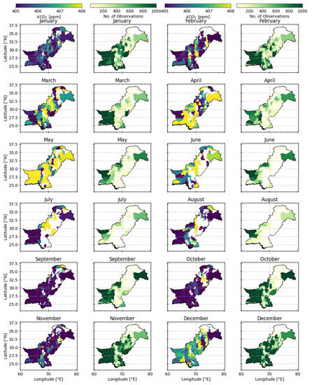
Figure 2.
Spatial distribution of monthly averaged XCO2 and the number of cloud-free OCO-2 retrievals in each district of Pakistan for a period of six years from January 2015 to December 2020.
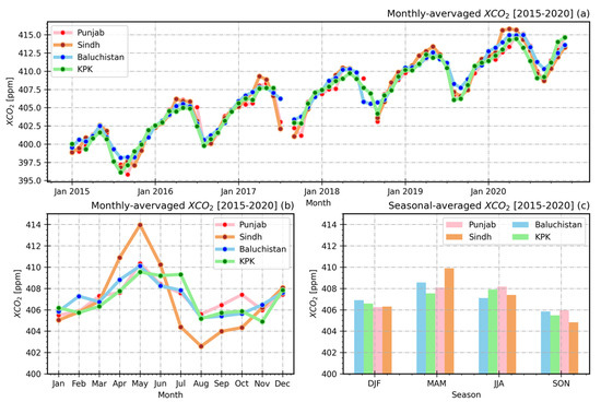
Figure 3.
(a) Long-term time series, (b) monthly averaged, and (c) seasonal-averaged XCO2 concentrations in various administrative units (provinces) of Pakistan derived using OCO-2 XCO2 retrievals from January 2015 to December 2020.
Figure 3 shows the long-term time series (Figure 3a), monthly averaged (Figure 3b), and seasonal-averaged concentrations (Figure 3c) of atmospheric CO2 over various administrative units of Pakistan including Punjab, Sindh, KPK, and Balochistan for a period of six years from 2015 to 2020. Gilgit Baltistan and Kashmir were not included in the analysis due to the insufficient number of OCO-2 retrievals. A similar varying trend of atmospheric CO2 concentration was observed in all the provinces of Pakistan; however, some differences were found in the magnitudes. The atmospheric CO2 concentrations during each month were higher than those in the same month of the previous year (Figure 3a). It reflected a continuous increase in CO2 concentrations. The seasonal-averaged XCO2 concentration of various provinces is shown in Figure 3c. Atmospheric CO2 concentration was higher during DJF and MAM, and lower in JJA, and SON. There was a slight difference between the magnitudes of seasonal-averaged XCO2 concentrations among the various provinces.
3.2. Spatial Distribution of MXCO2 and Anthropogenic CO2 Emissions
Figure 4b,c show the spatial distribution of the total number of cloud-free OCO-2 retrievals over a spatial grid of 0.5 × 0.5 degrees and within the district boundaries of Pakistan from 2015 to 2020. Overall, the number of observations was sufficient for most of the areas; however, the northern areas including Gilgit Baltistan and Kashmir received the lowest number of OCO-2 retrievals. Any district with observations of fewer than 300 retrievals was not considered in the study.
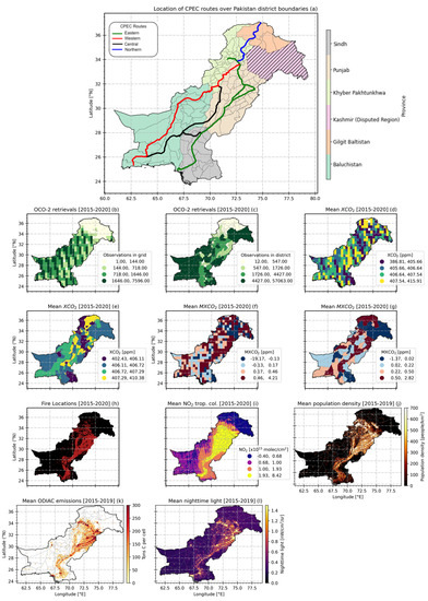
Figure 4.
(a) District and administrative unit boundaries of Pakistan along with the CPEC routes and spatial distribution of (b) OCO-2 retrievals over a grid of 0.5 × 0.5 degrees, (c) OCO-2 retrievals observed by each district, (d) mean XCO2 concentration over a grid of 0.5 × 0.5 degrees, (e) mean XCO2 concentration in each district, (f) mean MXCO2 concentration over a grid of 0.5 × 0.5 degrees, (g) mean MXCO2 concentration in each district, (h) fire locations, (i) mean NO2 tropospheric columns, (j) mean population density, (k) mean ODIAC emissions, and (l) mean nighttime lights over Pakistan.
Figure 4d,e show the annually averaged XCO2 concentration over a spatial grid of 0.5 × 0.5 degrees and within the district boundaries of Pakistan from 2015 to 2020. While the MXCO2 estimated using the OCO-2 retrievals is also displayed over a 0.5 × 0.5 degree spatial grid and the spatial boundaries of the districts (Figure 4f,g). MXCO2 represents anthropogenic CO2 concentrations. Surprisingly, higher MXCO2 concentrations were observed over the districts located along the China–Pakistan Economic Corridor (CPEC) routes shown in Figure 4a. Moreover, most of the districts in Punjab and Sindh are surrounded by cropland (Figure 1b). The spatial pattern of increased MXCO2 over Punjab and Sindh was somehow similar to that of the cropland (Figure 1b and Figure 4f,g). This higher concentration of MXCO2 over the cropland might be due to the pre- and post-harvest burning. A fire location product derived using the MODIS data from 2015 to 2020 is also shown in Figure 4h, which also exhibited a similar spatial distribution pattern. Moreover, NO2 is an indicator of atmospheric pollution, and it is co-emitted with CO2 when fossil fuels are combusted at high temperatures. It has a short lifetime on the order of hours, so NO2 columns often greatly exceed the background and noise levels of modern satellite sensors near sources, which makes it a suitable tracer of recently emitted CO2 [4]. Figure 4i shows the spatial distribution of mean NO2 tropospheric columns from 2015 to 2020. The spatial distribution pattern of increased NO2 is similar to that of MXCO2. Figure 4k shows the mean spatial distribution of anthropogenic CO2 emissions from 2015 to 2019 over Pakistan, estimated using the ODIAC dataset. The emission pattern showed that CO2 emissions were higher in Punjab followed by Sindh, KPK, and Balochistan. The anthropogenic emission pattern was similar to OCO-2-derived MXCO2 (Figure 4f,g,k) over Punjab and Sindh where the CO2 emissions were higher. However, this pattern was slightly different for other provinces where the emissions were lower. The mean nighttime lights dataset provided by the VIIRS from 2015 to 2019 is also displayed in Figure 4l. The results from both the ODIAC and nighttime light datasets showed similarities in spatial patterns as well as magnitudes. Moreover, the spatial distribution of the satellite-based MXCO2 (Figure 4f,g) was also compared with that of the population density (Figure 4j) and a similarity between the spatial distributions of the two datasets was observed. In summary, the MXCO2 derived using OCO-2 retrievals showed a spatial distribution pattern similar to cropland, fire locations, NO2 tropospheric column, population density, ODIAC emissions, and nighttime lights. To further determine the relationship of MXCO2 with these variables, statistical analyses were carried out between MXCO2 and other datasets including the population density and the NO2 tropospheric column, and the results are described in Section 3.3.
Figure 5a shows the multiyear mean XCO2 concentration in Pakistani districts. The results showed that the atmospheric CO2 concentration was continuously increasing in most of the districts. Figure 5b shows the mean MXCO2 concentrations in districts for five years from January 2015 to December 2019. The districts were ranked based on the mean MXCO2 concentration. The results showed that the districts with the highest concentrations of atmospheric CO2 were either among the most populous cities, industrial in nature or experiencing large-scale construction or economic activities. For instance, Karachi, the capital of Sindh, is the largest city in Pakistan with an estimated GDP of $164 billion (PPP) as of 2019 [57]. Being ranked as a beta-global city, Karachi is Pakistan’s premier industrial and economic hub with the two largest seaports, the Port of Karachi and Port Bin Qasim. Lahore is the second-largest city of Pakistan and the capital of Punjab with an estimated GDP of $65.14 billion (PPP) as of 2017 [58] and a projected average growth rate of 5.6% [22]. The ODIAC inventory v2019 suggested that Lahore whole-city CO2ff emissions increased by about 646 kt C/year during October 2014–May 2019, translating into a total change of 27% over 2015–2019 (i.e., a mean annual 5.9% increase), which is consistent with Pakistan’s national emission estimates of 5.05% during 2001–2018 [59]. Sialkot, Narowal, Nowshera, Multan, and Faisalabad are the cities where large-scale industrial activities are carried out. Islamabad is the capital of Pakistan. Kohistan and Mohmand were also listed among the districts with the highest MXCO2 concentrations. These cities contain large reservoir-based dams [60]. The reservoir-based dams emit a significant amount of CO2 into the atmosphere, and the dams located in tropical regions have even larger emissions compared to boreal and temperate regions [61]. Most of the districts showing the lowest MXCO2 concentrations were located in the Balochistan and KPK provinces. The districts located in KPK were mainly mountainous areas covered with forests (Figure 1b,c) and in the case of Balochistan, the districts with the lowest MXCO2 concentrations had the lowest population density, which indicated less human activity. Some districts, such as Umerkot, Mithi, and Mastung, belonging to the Sindh and Balochistan provinces, also had the lowest atmospheric CO2, and these districts were mainly covered with deserts. Figure 5c shows the annually averaged MXCO2 concentrations in districts of Pakistan from 2015 to 2019. The districts where MXCO2 concentrations were increasing were located in Punjab and Sindh; however, most of the districts with decreased annual concentrations were in the KPK and Balochistan provinces. In 2014, the government of KPK launched the Billion Tree Tsunami (BTT) project as a response to the challenge of global warming [62]. The project restored 350,000 hectares of forests and degraded land [63]. The BTT project was completed in August 2017, ahead of schedule. The decreased concentration of MXCO2 in KPK areas might be attributed to the large-scale afforestation; however, more evidence is needed to support the statement. Overall, as per the OCO-2 MXCO2 results, Punjab showed the highest MXCO2 concentration followed by Sindh, KPK, and Balochistan.
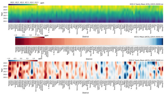
Figure 5.
(a) Mean annual concentration of XCO2, (b) ranking of cities based on mean MXCO2, and (c) mean annual MXCO2 concentration in districts of Pakistan.
Mean CO2 emissions for districts were also calculated and the districts were then ranked based on the amount of mean CO2 emissions (Figure 6a). The larger districts of Punjab and Sindh such as Karachi, Lahore, Multan, Muzaffargarh, Faisalabad, Rawalpindi, Hyderabad, and Dadu showed higher CO2 emissions. These districts were also listed among the ones with higher MXCO2 concentrations estimated using OCO-2 XCO2 retrievals (Figure 5b). These areas are among the most populated districts of Pakistan and experience large-scale economic activities. Based on the ODIAC CO2 emission dataset, most of the districts with the lowest amounts of CO2 emissions were located in Balochistan. The spatial distribution of the ODIAC dataset largely relies on nighttime lights, which result due to human activity. Balochistan is the largest province of Pakistan in terms of area with the lowest population density (Figure 4j). The low ODIAC CO2 emissions in districts located in Balochistan might be due to the lower population density, which results in producing fewer of the nighttime lights that primarily control the spatial distribution of the ODIAC emissions. Figure 6b shows the annually averaged CO2 emissions for each district of Pakistan, and the results show that CO2 emissions were continuously increasing in most of the districts located in the Punjab and Sindh provinces.
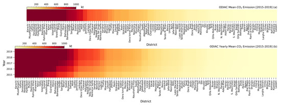
Figure 6.
(a) Ranking of Pakistani districts based on mean anthropogenic CO2 emissions and (b) mean annual anthropogenic CO2 emissions for a period of five years from 2015 to 2019.
3.3. Correlation Analysis
Figure 7 shows the correlation analysis of the OCO-2 MXCO2 and ODIAC CO2 emissions between each other and with some other datasets such as population density and the OMI NO2 tropospheric column. Population growth is one of the major causes of increased CO2 emissions in developed as well as developing countries, whereas the impact of population growth on CO2 emissions has not received enough attention. NO2 is an indicator of atmospheric pollution, and it is co-emitted with CO2 when fossil fuels are combusted at high temperatures.
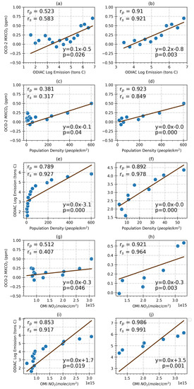
Figure 7.
(a) Scatterplot between ODIAC and OCO-2 anomalies (MXCO2), (b) scatterplot between ODIAC and OCO-2 anomalies at higher values, (c) scatterplot between OCO-2 and population density, (d) scatterplot between OCO-2 and population density at higher values, (e) scatterplot between ODIAC emissions and population density, (f) scatterplot between ODIAC emissions and population density at lower values, (g) scatterplot between OCO-2 and NO2 tropospheric column, (h) scatterplot between OCO-2 and NO2 tropospheric column at higher values, (i) scatterplot between ODIAC emissions and NO2 tropospheric column, and (j) scatterplot between ODIAC and NO2 tropospheric column at higher values. The Pearson and the Spearman correlations are represented by rp and rs, respectively.
Previous studies showed that compared to the single sounding of XCO2, clusters of satellite-based XCO2 retrievals showed a better and more significant correlation with other variables, which might be due to the fact that a single sounding is an instantaneous snapshot of the realistic atmosphere [41,48]. Therefore, we segmented the datasets and created clusters following the method described in [49] and then finally carried out correlation analyses between the datasets.
Figure 7a shows the scatterplot and correlation between ODIAC CO2 emissions and OCO-2 XCO2 anomalies (MXCO2). The two datasets showed correlation coefficients (rp represents Pearson’s correlation and rs represents Spearman’s correlation) of above 0.5, and this correlation was significantly improved (over 0.91) when the analysis was carried out between higher values of the two datasets (Figure 7b). Figure 7c shows the scatterplot and correlation between the OCO-2 anomalies and population density derived using the Landscan data. XCO2 anomalies showed a positive correlation with the population density, and this correlation was also improved when the analysis was carried out between higher values (Figure 7d). Figure 7e shows the scatterplot between the ODIAC emissions and the population density. ODIAC showed a relatively better correlation with the population density compared to OCO-2 XCO2 anomalies, and unlike OCO-2, the correlation between the ODIAC and population density was improved when the analysis was carried out after removing higher values (Figure 7f). However, both the OCO-2 and ODIAC datasets showed a positive correlation with the population density. Figure 7g shows the scatterplot and correlation between the XCO2 anomalies and NO2 tropospheric columns retrieved from OMI observations. Both of the datasets showed a positive correlation, and the correlation was improved when the analysis was carried out with higher values (Figure 7h). Hakkarainen et al. correlated OCO-2-based XCO2 anomalies with OMI NO2 tropospheric column over various regions and reported a good correlation between the two datasets [46]. Figure 7i,j show the scatterplot and correlation between the ODIAC CO2 emissions and NO2 tropospheric column, and both datasets showed a good correlation. The ODIAC dataset showed a better correlation with the NO2 tropospheric column compared to the OCO-2 XCO2 anomalies. In all the correlation analyses carried out between the OCO-2 XCO2 anomalies and other variables, the common results showed a relatively weaker correlation at lower values and the results significantly improved when the analyses were carried out with higher values.
4. Discussion
The temporal change in the quantity of satellite-based observations was more significant in the districts located in Punjab and Sindh. Pakistan is a monsoon-influenced country and generally, in Pakistan, March to May is treated as pre-monsoon, June to August as monsoon and September to November as post-monsoon season [2]. The rainy season in the country starts during the pre-monsoon period and meets the occurrence of the summer monsoon, from June to August, which is a major source of precipitation. The decreased number of OCO-2 soundings during the pre-monsoon and monsoon periods might be due to the presence of clouds, because the space-based observations are vulnerable to clouds and aerosols [33]. GOSAT and OCO-2 are processed using the ACOS FP algorithm that has evolved over time to improve the quality as well as the quantity of the retrievals. A recent study [64] showed that out of 37 million soundings collected by GOSAT through June 2020, only 5.4 % of the soundings (2 × 10⁶) were finally assigned a “good” XCO2 quality flag when processed using the ACOS FP algorithm, and other soundings were discarded due to the presence of clouds and other artefacts. Moreover, northern parts of the country including Gilgit Baltistan and Kashmir consistently had the lowest number of OCO-2 retrievals throughout the year. These areas are covered with the highest mountain ranges that are mostly covered with snow. The satellite observations over such complex areas showed larger uncertainties, did not meet the filtering criteria of the retrieval algorithms and were finally discarded.
The satellite-detected XCO2 anomaly (MXCO2) exhibited a spatial distribution similar to the CPEC route, NO2 tropospheric column, population density, fire location, cropland, and nighttime lights. The CPEC, a large-scale trading partnership between Pakistan and China, is a collection of infrastructure projects including a comprehensive road network connecting the Gwadar port to China [65,66,67]. Rapid development has been carried out on the CPEC project during the last decade. The notable works include the construction of the road network shown in Figure 4a, special economic zones along the CPEC routes, and several energy projects. The rapid development along the CPEC road network might be a potential reason for the increased levels of atmospheric CO2 concentration in the neighboring districts. NO2 is emitted when fossil fuels are burned at high temperatures, thus it is also an indicator of pollution. Hakkarainen et al. compared the spatial distribution of XCO2 anomalies derived using OCO-2 retrievals with that of NO2 tropospheric columns over various regions of the world and reported that both of the datasets showed similarities in terms of spatial distribution patterns [46,47]. In the case of the MXCO2–ODIAC comparison, similarity in the spatial distribution pattern of the two datasets was found over the areas which had higher anthropogenic emissions; however, some differences were also observed over the areas which had lower amounts of anthropogenic emissions. Several regional-scale studies have been carried out comparing the ODIAC CO2 emissions with the satellite-based XCO2 anomalies and reported that the ODIAC dataset showed a good agreement with satellite-based XCO2 concentration at higher values, whereas notable deviations occurred at lower values. Yang et al. studied the correlation between the ODIAC emissions and XCO2 anomalies derived using GOSAT retrievals over China and reported that the correlation between the two datasets was improved at higher values [48]. Similar results were reported by [41,46] when OCO-2-based XCO2 anomalies were compared with the ODIAC CO2 emissions. The differences between these two datasets are due to the different approaches to measurement. Bottom-up-approach-based inventories, i.e., ODIAC and CDIAC, estimate the CO2 emissions based on standardized protocols, combining activity data such as fuel production and consumption as well as traffic-monitoring data with pre-calculated emission factors for specific sources across different activity sectors. The datasets are distributed by either spatial proxies, i.e., nighttime lights, population density, or through combinations of line sources such as on-road emissions and point sources such as power plants [22]. ODIAC incorporates the nighttime lights and power plant point sources to produce a high-resolution CO2 emission dataset [37,38].
Furthermore, MXCO2 exhibited good correlations with various variables such as the ODIAC CO2 emissions, population density, and NO2 tropospheric columns at higher values; however, these correlations deteriorated at lower values. The larger deviation between smaller values of the datasets might be due to several reasons: (i) The ODIAC and population datasets may contain uncertainties due to data gaps, inaccurate calculation factors, inaccurate data, and the unavailability of statistics, especially for developing countries; (ii) uncertainties may be present in the XCO2 anomalies that are likely to be produced by the CO2 uptake of the biosphere, which remains in the XCO2 anomalies.
5. Summary and Conclusions
In this work, we used OCO-2 and the ODIAC CO2 datasets to study the scenario of CO2 over 120 districts of Pakistan. The spatial coverage of OCO-2, spatial distribution, and monthly and seasonal variations of atmospheric CO2 were studied in detail. OCO-2 provided a reasonable spatial coverage over Pakistan except for the northern areas, which are mostly covered with the highest mountain ranges. Moreover, the quantity of OCO-2 retrievals started decreasing during the pre-monsoon season and reached the minimum during the monsoon season (June to August). This might be due to the presence of clouds that strongly affected the space-borne observations. The concentration of atmospheric CO2 was continuously increasing in Pakistan with significant seasonal fluctuations. The maximum and minimum concentrations of atmospheric CO2 were observed in May and September, respectively. Moreover, the atmospheric CO2 concentration was higher during DJF and MAM, and lower in JJA and SON. A slight difference in the concentration of atmospheric CO2 was also observed between various administrative units of Pakistan.
To study the anthropogenic CO2 using a satellite dataset, OCO-2 retrievals were deseasonalized and detrended by calculating the XCO2 anomalies (MXCO2). The spatial distribution pattern of MXCO2 showed higher concentrations over the cities located along the CPEC routes. The spatial distribution pattern of the satellite-based MXCO2 was compared with those of various datasets including the ODIAC CO2 emissions, OMI NO2 tropospheric column, population density, nighttime lights, fire locations, and cropland, and all the datasets showed a similarity in the spatial distribution pattern. Mean MXCO2 concentrations were calculated within the spatial boundaries of districts, and the districts were then ranked based on the mean MXCO2 concentrations. The cities showing the highest MXCO2 concentrations were either metropolitan cities or experiencing large-scale economic activities. Karachi, Lahore, Faisalabad, Multan, Sialkot and Narowal were among the cities with the highest MXCO2 concentrations. The cities with the lowest MXCO2 concentrations were mostly located in the KPK and Balochistan provinces. Moreover, Punjab showed the highest anthropogenic CO2 concentration among the administrative units, followed by Sindh, KPK, and Balochistan.
Anthropogenic CO2 emissions over Pakistan were studied using the ODIAC dataset. The spatial distribution pattern of the ODIAC emissions was also similar to those of the satellite-derived MXCO2, OMI NO2 tropospheric column, and population density. The ODIAC spatial distribution pattern showed some deviations from that of the satellite-derived MXCO2 over the areas where population density was significantly low. This might be due to the fact that the ODIAC dataset largely relied on nighttime lights for the spatial distribution, and nighttime light is difficult to detect from a satellite over the areas with lower human activity. To determine the anthropogenic CO2 emissions in each district, the mean CO2 emissions were estimated for each of the districts, and the districts were then ranked based on the mean CO2 emissions. The districts with the highest MXCO2 concentrations such as Karachi, Lahore, Muzaffargarh, Multan, Faisalabad, and Rawalpindi were also among the cities with the highest CO2 emissions. The results showed that CO2 emissions were increasing in most of the cities.
The spatial distribution patterns of the satellite-derived MXCO2 and ODIAC CO2 emissions showed a similar trend with the population density and NO2 tropospheric column. Therefore, to study the relationship between various variables, cluster-based correlation analyses were carried out. The results showed that OCO-2 MXCO2 showed a positive and significant correlation with the ODIAC CO2 emissions, and these correlations improved when the analysis was carried out with higher values. Both the OCO-2 and ODIAC datasets showed positive and significant correlations with the NO2 tropospheric column and population density. The common results of OCO-2 MXCO2 with all the variables showed that the correlation was improved when the smaller values were removed. This might be due to the uncertainties in the MXCO2 caused by CO2 uptake of the biosphere or atmospheric transport. However, the matter needs further investigation.
Several satellites are now orbiting around the earth and continuously monitoring atmospheric CO2. In the future, we intend to study the potential of joint utilization of multiple CO2-monitoring satellite datasets along with atmospheric transport modeling to monitor the atmospheric CO2 at local scales.
Author Contributions
Conceptualization, F.M.; Methodology, F.M.; Software, L.B.; Formal analysis, F.M.; Data curation, F.M., L.B., Q.W., M.S., M.B., S.U. and Z.F.; Writing—original draft, F.M.; Writing—review & editing, L.B., N.A., M.X. and M.S.; Supervision, L.B.; Funding acquisition, L.B. All authors have read and agreed to the published version of the manuscript.
Funding
This work was supported by the National Natural Science Foundation of China (Grant No. 42175145), Shanghai Aerospace Science and Technology Innovation Foundation (SAST 2019-045), and the Qinglan Project of Jiangsu Province of China.
Data Availability Statement
Links to the datasets used in this study have been provided in the Datasets section of the manuscript.
Acknowledgments
The authors acknowledge the efforts of NASA to provide the OCO-2 data products. These data were produced by the OCO-2 project at the Jet Propulsion Laboratory, California Institute of Technology, and obtained from the OCO-2 data archive maintained at the NASA Goddard Earth Science Data and Information Services Center. The authors are highly grateful to the NIES for providing ODIAC anthropogenic emission dataset. Furthermore, the authors are also thankful to the organizations providing several other datasets used in the study such as, MODIS products, Oak Ridge National Laboratory population density dataset, OMI NO2 dataset, VIIRS nighttime lights dataset, and the Copernicus landcover dataset.
Conflicts of Interest
The authors declare that there is no conflict of interest.
References
- IPCC. Climate Change 2013—The Physical Science Basis; Intergovernmental Panel on Climate Change, Ed.; Cambridge University Press: Cambridge, UK, 2014; Volume 9781107057, ISBN 9781107415324. [Google Scholar]
- Mustafa, F.; Bu, L.; Wang, Q.; Ali, M.A.; Bilal, M.; Shahzaman, M.; Qiu, Z. Multi-Year Comparison of CO2 Concentration from NOAA Carbon Tracker Reanalysis Model with Data from GOSAT and OCO-2 over Asia. Remote Sens. 2020, 12, 2498. [Google Scholar] [CrossRef]
- Hoegh-Guldberg, O.; Jacob, D.; Bindi, M.; Brown, S.; Camilloni, I.; Diedhiou, A.; Djalante, R.; Ebi, K.; Engelbrecht, F.; Guiot, J.; et al. Impacts of 1.5 C Global Warming on Natural and Human Systems. In Global Warming of 1.5 °C. An IPCC Special Report. 2018. Available online: https://www.ipcc.ch/site/assets/uploads/sites/2/2019/02/SR15_Chapter3_Low_Res.pdf (accessed on 11 August 2022).
- Reuter, M.; Buchwitz, M.; Schneising, O.; Krautwurst, S.; O’Dell, C.W.; Richter, A.; Bovensmann, H.; Burrows, J.P. Towards Monitoring Localized CO Emissions from Space: Co-Located Regional CO2 and NO2 Enhancements Observed by the OCO-2 and S5P Satellite. Atmos. Chem. Phys. 2019, 19, 9371–9383. [Google Scholar] [CrossRef]
- Ciais, P.; Dolman, A.J.; Bombelli, A.; Duren, R.; Peregon, A.; Rayner, P.J.; Miller, C.; Gobron, N.; Kinderman, G.; Marland, G.; et al. Current Systematic Carbon-Cycle Observations and the Need for Implementing a Policy-Relevant Carbon Observing System. Biogeosciences 2014, 11, 3547–3602. [Google Scholar] [CrossRef]
- Schultz, M.G.; Akimoto, H.; Bottenheim, J.; Buchmann, B.; Galbally, I.E.; Gilge, S.; Helmig, D.; Koide, H.; Lewis, A.C.; Novelli, P.C.; et al. The Global Atmosphere Watch Reactive Gases Measurement Network. Elementa 2015, 3, 1–23. [Google Scholar] [CrossRef]
- Frey, M.; Sha, M.K.; Hase, F.; Kiel, M.; Blumenstock, T.; Harig, R.; Surawicz, G.; Deutscher, N.M.; Shiomi, K.; Franklin, J.E.; et al. Building the COllaborative Carbon Column Observing Network (COCCON): Long-Term Stability and Ensemble Performance of the EM27/SUN Fourier Transform Spectrometer. Atmos. Meas. Tech. 2019, 12, 1513–1530. [Google Scholar] [CrossRef]
- Velazco, V.A.; Deutscher, N.M.; Morino, I.; Uchino, O.; Bukosa, B.; Ajiro, M.; Kamei, A.; Jones, N.B.; Paton-Walsh, C.; Griffith, D.W.T. Satellite and Ground-Based Measurements of XCO2 in a Remote Semiarid Region of Australia. Earth Syst. Sci. Data 2019, 11, 935–946. [Google Scholar] [CrossRef]
- Toon, G.; Blavier, J.-F.; Washenfelder, R.; Wunch, D.; Keppel-Aleks, G.; Wennberg, P.; Connor, B.; Sherlock, V.; Griffith, D.; Deutscher, N.; et al. Total Column Carbon Observing Network (TCCON). In Proceedings of the Advances in Imaging, Vancouver, BC, Canada, 26–30 April 2009; p. JMA3. Available online: https://opg.optica.org/abstract.cfm?URI=FTS-2009-JMA3 (accessed on 11 August 2022).
- Wang, Q.; Mustafa, F.; Bu, L.; Yang, J.; Fan, C.; Liu, J.; Chen, W. Monitoring of Atmospheric Carbon Dioxide over a Desert Site Using Airborne and Ground Measurements. Remote Sens. 2022, 14, 5224. [Google Scholar] [CrossRef]
- Grieco, G.; Masiello, G.; Serio, C.; Jones, R.L.; Mead, M.I. Infrared Atmospheric Sounding Interferometer Correlation Interferometry for the Retrieval of Atmospheric Gases: The Case of H2O and CO2. Appl. Opt. 2011, 50, 4516. [Google Scholar] [CrossRef]
- Crevoisier, C.; Heilliette, S.; Chédin, A.; Serrar, S.; Armante, R.; Scott, N.A. Midtropospheric CO2 Concentration Retrieval from AIRS Observations in the Tropics. Geophys. Res. Lett. 2004, 31, 17. [Google Scholar] [CrossRef]
- Engelen, R.J. Estimating Atmospheric CO2 from Advanced Infrared Satellite Radiances within an Operational 4D-Var Data Assimilation System: Methodology and First Results. J. Geophys. Res. 2004, 109, D19309. [Google Scholar] [CrossRef]
- Buchwitz, M.; de Beek, R.; Noël, S.; Burrows, J.P.; Bovensmann, H.; Bremer, H.; Bergamaschi, P.; Körner, S.; Heimann, M. Carbon Monoxide, Methane and Carbon Dioxide Columns Retrieved from SCIAMACHY by WFM-DOAS: Year 2003 Initial Data Set. Atmos. Chem. Phys. 2005, 5, 3313–3329. [Google Scholar] [CrossRef]
- Kuze, A.; Suto, H.; Nakajima, M.; Hamazaki, T. Thermal and near Infrared Sensor for Carbon Observation Fourier-Transform Spectrometer on the Greenhouse Gases Observing Satellite for Greenhouse Gases Monitoring. Appl. Opt. 2009, 48, 6716–6733. [Google Scholar] [CrossRef] [PubMed]
- Liu, Y.; Wang, J.; Yao, L.; Chen, X.; Cai, Z.; Yang, D.; Yin, Z.; Gu, S.; Tian, L.; Lu, N.; et al. The TanSat Mission: Preliminary Global Observations. Sci. Bull. 2018, 63, 1200–1207. [Google Scholar] [CrossRef]
- Matsunaga, T.; Morino, I.; Yoshida, Y.; Saito, M.; Noda, H.; Ohyama, H.; Niwa, Y.; Yashiro, H.; Kamei, A.; Kawazoe, F.; et al. Early Results of GOSAT-2 Level 2 Products. In Proceedings of the AGU Fall Meeting Abstracts, San Francisco, CA, USA, 9–13 December 2019; Volume 2019, p. A52H-02. [Google Scholar]
- Eldering, A.; Taylor, T.E.; O’Dell, C.W.; Pavlick, R. The OCO-3 Mission: Measurement Objectives and Expected Performance Based on 1 Year of Simulated Data. Atmos. Meas. Tech. 2019, 12, 2341–2370. [Google Scholar] [CrossRef]
- Eckstein, D.; Künzel, V.; Schäfer, L. Global Climate Risk Index 2021; Germanwatch: Berlin, Germany, 2021; pp. 13–14. Available online: https://germanwatch.org/sites/default/files/Global%20Climate%20Risk%20Index%202021_1.pdf (accessed on 11 August 2022).
- Eldering, A.; Wennberg, P.O.; Crisp, D.; Schimel, D.S.; Gunson, M.R.; Chatterjee, A.; Liu, J.; Schwandner, F.M.; Sun, Y.; O’Dell, C.W.; et al. The Orbiting Carbon Observatory-2 Early Science Investigations of Regional Carbon Dioxide Fluxes. Science 2017, 358, eaam5745. [Google Scholar] [CrossRef]
- Shim, C.; Han, J.; Henze, D.K.; Yoon, T. Identifying Local Anthropogenic CO2 Emissions with Satellite Retrievals: A Case Study in South Korea. Int. J. Remote Sens. 2019, 40, 1011–1029. [Google Scholar] [CrossRef]
- Lei, R.; Feng, S.; Danjou, A.; Broquet, G.; Wu, D.; Lin, J.C.; O’Dell, C.W.; Lauvaux, T. Fossil Fuel CO2 Emissions over Metropolitan Areas from Space: A Multi-Model Analysis of OCO-2 Data over Lahore, Pakistan. Remote Sens. Environ. 2021, 264, 112625. [Google Scholar] [CrossRef]
- Wu, D.; Lin, J.C.; Oda, T.; Kort, E.A. Space-Based Quantification of per Capita CO2 Emissions from Cities. Environ. Res. Lett. 2020, 15, 035004. [Google Scholar] [CrossRef]
- Labzovskii, L.D.; Jeong, S.-J.; Parazoo, N.C. Working towards Confident Spaceborne Monitoring of Carbon Emissions from Cities Using Orbiting Carbon Observatory-2. Remote Sens. Environ. 2019, 233, 111359. [Google Scholar] [CrossRef]
- Nassar, R.; Hill, T.G.; McLinden, C.A.; Wunch, D.; Jones, D.B.A.; Crisp, D. Quantifying CO2 Emissions From Individual Power Plants From Space. Geophys. Res. Lett. 2017, 44, 10045–10053. [Google Scholar] [CrossRef]
- Bilal, M.; Mhawish, A.; Nichol, J.E.; Qiu, Z.; Nazeer, M.; Ali, A.; de Leeuw, G.; Levy, R.C.; Wang, Y.; Chen, Y.; et al. Air Pollution Scenario over Pakistan: Characterization and Ranking of Extremely Polluted Cities Using Long-Term Concentrations of Aerosols and Trace Gases. Remote Sens. Environ. 2021, 264, 112617. [Google Scholar] [CrossRef]
- Crisp, D.; Miller, C.E.; DeCola, P.L. NASA Orbiting Carbon Observatory: Measuring the Column Averaged Carbon Dioxide Mole Fraction from Space. J. Appl. Remote Sens. 2008, 2, 023508. [Google Scholar] [CrossRef]
- Crisp, D.; Pollock, H.; Rosenberg, R.; Chapsky, L.; Lee, R.; Oyafuso, F.; Frankenberg, C.; Dell, C.; Bruegge, C.; Doran, G.; et al. The On-Orbit Performance of the Orbiting Carbon Observatory-2 (OCO-2) Instrument and Its Radiometrically Calibrated Products. Atmos. Meas. Tech. 2017, 10, 59–81. [Google Scholar] [CrossRef]
- O’Dell, C.W.; Connor, B.; Bösch, H.; O’Brien, D.; Frankenberg, C.; Castano, R.; Christi, M.; Eldering, D.; Fisher, B.; Gunson, M.; et al. The ACOS CO2 Retrieval Algorithm-Part 1: Description and Validation against Synthetic Observations. Atmos. Meas. Tech. 2012, 5, 99–121. [Google Scholar] [CrossRef]
- Crisp, D.; Fisher, B.M.; O’Dell, C.; Frankenberg, C.; Basilio, R.; Bösch, H.; Brown, L.R.; Castano, R.; Connor, B.; Deutscher, N.M.; et al. The ACOS CO2 Retrieval Algorithm—Part II: Global X CO2 Data Characterization. Atmos. Meas. Tech. 2012, 5, 687–707. [Google Scholar] [CrossRef]
- Wunch, D.; Wennberg, P.O.; Osterman, G.; Fisher, B.; Naylor, B.; Roehl, M.C.; O’Dell, C.; Mandrake, L.; Viatte, C.; Kiel, M.; et al. Comparisons of the Orbiting Carbon Observatory-2 (OCO-2) XCO2 Measurements with TCCON. Atmos. Meas. Tech. 2017, 10, 2209–2238. [Google Scholar] [CrossRef]
- O’Dell, C.W.; Eldering, A.; Wennberg, P.O.; Crisp, D.; Gunson, M.R.; Fisher, B.; Frankenberg, C.; Kiel, M.; Lindqvist, H.; Mandrake, L.; et al. Improved Retrievals of Carbon Dioxide from Orbiting Carbon Observatory-2 with the Version 8 ACOS Algorithm. Atmos. Meas. Tech. 2018, 11, 6539–6576. [Google Scholar] [CrossRef]
- Kiel, M.; Dell, C.W.O.; Fisher, B.; Eldering, A.; Nassar, R.; Macdonald, C.G.; Wennberg, P.O.; O’Dell, C.W.; Fisher, B.; Eldering, A.; et al. How Bias Correction Goes Wrong: Measurement of XCO2 Affected by Erroneous Surface Pressure Estimates. Atmos. Meas. Tech. 2019, 12, 2241–2259. [Google Scholar] [CrossRef]
- Mustafa, F.; Wang, H.; Bu, L.; Wang, Q.; Shahzaman, M.; Bilal, M.; Zhou, M.; Iqbal, R.; Aslam, R.; Ali, A.; et al. Validation of GOSAT and OCO-2 against In Situ Aircraft Measurements and Comparison with CarbonTracker and GEOS-Chem over Qinhuangdao, China. Remote Sens. 2021, 13, 899. [Google Scholar] [CrossRef]
- ODell, C.; Eldering, A.; Gunson, M.; Crisp, D.; Fisher, B.; Kiel, M.; Kuai, L.; Laughner, J.; Merrelli, A.; Nelson, R.; et al. Improvements in XCO2 Accuracy from OCO-2 with the Latest ACOS V10 Product; 2021; p. EGU21-10484. Available online: https://doi.org/10.5194/egusphere-egu21-10484 (accessed on 11 August 2022). [CrossRef]
- Oda, T.; Maksyutov, S. A Very High-Resolution (1 Km × 1 Km) Global Fossil Fuel CO2 Emission Inventory Derived Using a Point Source Database and Satellite Observations of Nighttime Lights. Atmos. Chem. Phys. 2011, 11, 543–556. [Google Scholar] [CrossRef]
- Oda, T.; Maksyutov, S.; Andres, R.J. The Open-Source Data Inventory for Anthropogenic CO2 Version 2016 (ODIAC2016): A Global Monthly Fossil Fuel CO2 Gridded Emissions Data Product for Tracer Transport Simulations and Surface Flux Inversions. Earth Syst. Sci. Data 2018, 10, 87–107. [Google Scholar] [CrossRef] [PubMed]
- Oda, T. ODIAC Fossil Fuel CO2 Emissions Dataset 2015; Center for Global Environmental Research, National Institute for Environmental Studies: Tsukuba, Ibaraki, Japan, 2015. [Google Scholar] [CrossRef]
- Boden, T.A.; Andres, R.J.; Marland, G. Environmental System Science Data Infrastructure for a Virtual Ecosystem. In Global, Regional, and National Fossil-Fuel CO2 Emissions (1751–2014) (v. 2017); Oak Ridge National Laboratory, U.S. Department of Energy: Oak Ridge, Tenn, USA, 2017. Available online: https://cdiac.ess-dive.lbl.gov/trends/emis/overview_2014.html (accessed on 11 August 2022).
- Chen, J.; Zhao, F.; Zeng, N.; Oda, T. Comparing a Global High-Resolution Downscaled Fossil Fuel CO2 Emission Dataset to Local Inventory-Based Estimates over 14 Global Cities. Carbon Balance Manag. 2020, 15, 9. [Google Scholar] [CrossRef] [PubMed]
- Mustafa, F.; Bu, L.; Wang, Q.; Yao, N.; Shahzaman, M.; Bilal, M.; Aslam, R.W.; Iqbal, R. Neural-Network-Based Estimation of Regional-Scale Anthropogenic CO2 Emissions Using an Orbiting Carbon Observatory-2 (OCO-2) Dataset over East and West Asia. Atmos. Meas. Tech. 2021, 14, 7277–7290. [Google Scholar] [CrossRef]
- Krotkov, N.A.; Veefkind, P. OMI/Aura Nitrogen Dioxide (NO2) Total and Tropospheric Column 1-Orbit L2 Swath 13 × 24 Km; Goddard Earth Sciences Data and Information Services Center (GES DISC): Greenbelt, MD, USA, 2012. [Google Scholar]
- Elvidge, C.D.; Zhizhin, M.; Ghosh, T.; Hsu, F.-C.; Taneja, J. Annual Time Series of Global VIIRS Nighttime Lights Derived from Monthly Averages: 2012 to 2019. Remote Sens. 2021, 13, 922. [Google Scholar] [CrossRef]
- Bright, E.A.; Rose, A.N.; Urban, M.L.; McKee, J. LandScan 2017 High-Resolution Global Population Data Set; Oak Ridge National Laboratory: Oak Ridge, TN, USA, 2018. [Google Scholar] [CrossRef]
- Buchhorn, M.; Lesiv, M.; Tsendbazar, N.-E.; Herold, M.; Bertels, L.; Smets, B. Copernicus Global Land Cover Layers—Collection 2. Remote Sens. 2020, 12, 1044. [Google Scholar] [CrossRef]
- Hakkarainen, J.; Ialongo, I.; Tamminen, J. Direct Space-based Observations of Anthropogenic CO2 Emission Areas from OCO-2. Geophys. Res. Lett. 2016, 43, 11400–11406. [Google Scholar] [CrossRef]
- Hakkarainen, J.; Ialongo, I.; Maksyutov, S.; Crisp, D. Analysis of Four Years of Global XCO2 Anomalies as Seen by Orbiting Carbon Observatory-2. Remote Sens. 2019, 11, 850. [Google Scholar] [CrossRef]
- Yang, S.; Lei, L.; Zeng, Z.; He, Z.; Zhong, H. An Assessment of Anthropogenic CO2 Emissions by Satellite-Based Observations in China. Sensors 2019, 19, 1118. [Google Scholar] [CrossRef]
- Mustafa, F.; Bu, L.; Wang, Q.; Shahzaman, M.; Bilal, M.; Aslam, R.W.; Dong, C. Spatiotemporal Investigation of Near-Surface CO2 and Its Affecting Factors over Asia. IEEE Trans. Geosci. Remote Sens. 2022, 60, 1–16. [Google Scholar] [CrossRef]
- Anthwal, A.; Joshi, V.; Joshi, S.C.C.; Sharma, A.; Kim, K.-H. Atmospheric Carbon Dioxide Levels in Garhwal Himalaya, India. J. Korean Earth Sci. Soc. 2009, 30, 588–597. [Google Scholar] [CrossRef][Green Version]
- Sreenivas, G.; Mahesh, P.; Subin, J.; Kanchana, A.L.; Rao, P.V.N.; Dadhwal, V.K. Influence of Meteorology and Interrelationship with Greenhouse Gases (CO2 and CH4) at a Suburban Site of India. Atmos. Chem. Phys. 2016, 16, 3953–3967. [Google Scholar] [CrossRef]
- Fang, S.X.; Zhou, L.X.; Tans, P.P.; Ciais, P.; Steinbacher, M.; Xu, L.; Luan, T. In Situ Measurement of Atmospheric CO2 at the Four WMO/GAW Stations in China. Atmos. Chem. Phys. 2014, 14, 2541–2554. [Google Scholar] [CrossRef]
- Sharma, N.; Nayak, R.K.; Dadhwal, V.K.; Kant, Y.; Ali, M.M. Temporal Variations of Atmospheric CO2 in Dehradun, India during 2009. Air Soil Water Res. 2012, 6, 37–45. [Google Scholar] [CrossRef]
- Golkar, F.; Al-Wardy, M.; Saffari, S.F.; Al-Aufi, K.; Al-Rawas, G. Using OCO-2 Satellite Data for Investigating the Variability of Atmospheric CO2 Concentration in Relationship with Precipitation, Relative Humidity, and Vegetation over Oman. Water 2019, 12, 101. [Google Scholar] [CrossRef]
- Kirschke, S.; Bousquet, P.; Ciais, P.; Saunois, M.; Canadell, J.G.; Dlugokencky, E.J.; Bergamaschi, P.; Bergmann, D.; Blake, D.R.; Bruhwiler, L.; et al. Three Decades of Global Methane Sources and Sinks. Nat. Geosci. 2013, 6, 813–823. [Google Scholar] [CrossRef]
- Nalini, K.; Uma, K.N.; Sijikumar, S.; Tiwari, Y.K.; Ramachandran, R. Satellite- and Ground-Based Measurements of CO2 over the Indian Region: Its Seasonal Dependencies, Spatial Variability, and Model Estimates. Int. J. Remote Sens. 2018, 39, 7881–7900. [Google Scholar] [CrossRef]
- Finance Division Pakistan. Pakistan Economic Survey 2018–2019; Finance Division, Government of Pakistan, 44000 Islamabad, Pakistan: 2019. Available online: https://finance.gov.pk/survey/chapters_19/Economic_Survey_2018_19.pdf (accessed on 12 March 2022).
- InpaperMagazine 2018. Available online: https://www.dawn.com/news/1382881 (accessed on 14 April 2022).
- Lei, R.; Feng, S.; Lauvaux, T. Country-Scale Trends in Air Pollution and Fossil Fuel CO2 Emissions during 2001–2018: Confronting the Roles of National Policies and Economic Growth. Environ. Res. Lett. 2021, 16, 014006. [Google Scholar] [CrossRef]
- Energy, N. 2018. Available online: https://www.nsenergybusiness.com/projects/diamer-bhasha-dam-hydropower-project/ (accessed on 14 April 2022).
- Graham-Rowe, D. 2005. Available online: https://www.newscientist.com/article/dn7046-hydroelectric-powers-dirty-secret-revealed/ (accessed on 20 March 2022).
- Kamal, A.; Yingjie, M.; Ali, A. Significance of Billion Tree Tsunami Afforestation Project and Legal Developments in Forest Sector of Pakistan. Int. J. Law Soc. 2019, 1, 157–165. [Google Scholar] [CrossRef]
- World Economic Forum. Pakistan Has Planted over a Billion Trees; World Economic Forum: Cologny, Switzerland, 2018; Available online: https://www.weforum.org/agenda/2018/07/pakistan-s-billion-tree-tsunami-is-astonishing (accessed on 21 April 2022).
- Taylor, T.E.; O’Dell, C.W.; Crisp, D.; Kuze, A.; Lindqvist, H.; Wennberg, P.O.; Chatterjee, A.; Gunson, M.; Eldering, A.; Fisher, B.; et al. An Eleven Year Record of XCO2 Estimates Derived from GOSAT Measurements Using the NASA ACOS Version 9 Retrieval Algorithm. In Atmosphere—Atmospheric Chemistry and Physics. 2021. Available online: https://doi.org/10.5194/essd-14-325-2022 (accessed on 11 August 2022). [CrossRef]
- Saad, A.; Ijaz, M.; Asghar, M.U.; Yamin, L. China-Pakistan Economic Corridor and Its Impact on Rural Development and Human Life Sustainability. Observations from Rural Women. PLoS ONE 2020, 15, e0239546. [Google Scholar] [CrossRef]
- Ullah, S.; You, Q.; Ullah, W.; Hagan, D.F.T.; Ali, A.; Ali, G.; Zhang, Y.; Jan, M.A.; Bhatti, A.S.; Xie, W. Daytime and Nighttime Heat Wave Characteristics Based on Multiple Indices over the China–Pakistan Economic Corridor. Clim. Dyn. 2019, 53, 6329–6349. [Google Scholar] [CrossRef]
- Ullah, S.; You, Q.; Ali, A.; Ullah, W.; Jan, M.A.; Zhang, Y.; Xie, W.; Xie, X. Observed Changes in Maximum and Minimum Temperatures over China-Pakistan Economic Corridor during 1980–2016. Atmos. Res. 2019, 216, 37–51. [Google Scholar] [CrossRef]


Publisher’s Note: MDPI stays neutral with regard to jurisdictional claims in published maps and institutional affiliations. |
© 2022 by the authors. Licensee MDPI, Basel, Switzerland. This article is an open access article distributed under the terms and conditions of the Creative Commons Attribution (CC BY) license (https://creativecommons.org/licenses/by/4.0/).