Abstract
Supraglacial lakes (SGL) are a specific phenomenon of glaciers. They are important for ice dynamics, surface mass balance, and surface hydrology, especially during ongoing climate changes. The important characteristics of lakes are their water storage and drainage. Satellite-based remote sensing is commonly used not only to monitor the area but also to estimate the depth and volume of lakes, which is the basis for long-term spatiotemporal analysis of these phenomena. Lake depth retrieval from optical data using a physical model requires several basic assumptions such as, for instance, the water has little or no dissolved or suspended matter. Several authors using these assumptions state that they are also potential weaknesses, which remain unquantified in the literature. The objective of this study is to quantify the effect of maximum detectable lake depth for water with non-zero suspended particulate matter (SPM). We collected in-situ concurrent measurements of hyperspectral and lake depth observations to a depth of 8 m. Additionally, we collected water samples to measure the concentration of SPM. The results of empirical and physically based models proved that a good relationship still exists between the water spectra of SGL and the lake depth in the presence of 48 mg/L of SPM. The root mean squared error for the models ranged from 0.163 m (Partial Least Squares Regression—PLSR model) to 0.243 m (physically based model), which is consistent with the published literature. However, the SPM limited the maximum detectable depth to approximately 3 m. This maximum detectable depth was also confirmed by the theoretical concept of Philpot (1989). The maximum detectable depth decreases exponentially with an increase in the water attenuation coefficient g, which directly depends on the water properties.
1. Introduction
Supraglacial lakes (SGLs) are an important phenomenon of the cryosphere for several reasons even though they are rather small and shallow (compared to other types of lakes around the world) and are bound to specific environments both on ice sheets and on mountain glacier tongues. The current literature about SGLs is abundant with references to the strong deglaciation of the ice sheets and mountain glacier tongues (and its reaction to climate change), and to glacier related hazards (e.g., Glacial Lake Outburst Floods—GLOF). The importance of supraglacial lakes has substantially changed in recent decades. In the middle of the last century, supraglacial lakes were considered as ephemeral phenomena that were interesting only as limnological curiosities [1]. Supraglacial lakes are those that develop directly on the glacier [2]. Melting of ice may result in the development of SGLs due to glacier ablation and its interaction with the drainage system [3]. The spatial distribution of supraglacial lakes on a glacier is constrained by thermal conditions, glacier surface inclination, and debris cover [4]. The upper limit is defined by the zero isotherm during the melt season, while the lower limit represents the glacier terminus [5,6]. Nevertheless, the lower limit could be influenced by thick debris cover, which prevents melting, and the lowermost end could in this way be shifted upslope the glacier [5]. Liu et al. [7] described the impact of debris cover and mean air temperature on the supraglacial lake distribution based on studies from Tien-Shan. Parts of the article from Emmer et al. [8] describe the cycle of formation and extinction of supraglacial lakes and the melting of buried (debris-covered) ice.
Over the last two decades, SGLs have attracted attention due to their formation and expansion due to climate change [5,9,10,11]. The influence of ice melts and ice flow on the Greenland ice sheet, and potentially their causal role in ice shelf disintegration on the Antarctic Peninsula, was mentioned by Langley et al. [12]. Banwell et al. [13] stressed that supraglacial meltwater lakes trigger ice-shelf break-up and modulate seasonal icesheet flow and are therefore agents by which warming is transmitted to the Antarctic and Greenland ice sheets. The influence on heat transport is also mentioned (apart from surface mass balance and ice dynamics) in the publication by Pope et al. [14]. The SGLs and their outbursts substantially affect the net ablation rate of glaciers [15], having a great impact on its mass and water balance [6]. Everett et al. [16] pointed out that observations on the west coast of the Greenland ice sheet typically show an up-glacier progression of drainage as the annual melt extent spreads inland.
Publications relating the formation and rapid drainage of SGLs to the mass balance and dynamics of glaciers [17,18,19,20,21,22] have become increasingly more common in recent years [23,24,25]. SGLs certainly affect not only the subglacial conditions but also the surface glacier environment [26]. Nevertheless, the sudden drainage of SGLs has been previously observed to initiate surface-to-bed hydrologic connections, which can enhance basal sliding in regions of the Greenland ice sheet where ice thickness approaches 1.0 km [27].
Due to global warming and following glacier retreat, new lakes are developed [28]. SGLs are usually not part of glacial lake inventories, because they are rather small and shallow (e.g., Baťka et al. [29]). Nevertheless, they may contribute to the glacial lake outburst floods (GLOFs) hazard. It is therefore important to understand the role of SGLs in glaciated areas, i.e., where these lakes are, what volume of water they store, when they form, and how they change over the melting season and over long time periods. SGLs are usually rather unstable, and this is one of the reasons why we need to understand the processes of origin and formation and their depth and volume.
Satellite-based remote sensing is commonly used to detect the location, area, and depth (volume) of SGLs. Numerous studies confirm the high accuracy of SGL detection and tracking [21,27,30]. For instance, Liang et al. [27] reported an accuracy of 99.0% for the detection of the area of SGLs, while the accuracy of the tracking was 96.3%. Dirscherl et al. [31] reported a F1-score of up to 98%, while the average F1-score was 86% using Sentinel-2 optical images. Moussavi et al. [32] combined Landsat-8 and Sentinel-2 imagery and achieved overall accuracies of >95% for Landsat-8 and >97% for Sentinel-2. Recently, research studies have been published that also use Synthetic Aperture Radar (SAR) images [25,33] to increase the temporal resolution in periods of dense clouds. However, the accuracy of the detection of the SGL extent has not yet been compared with the optical data.
Lake properties such as lake area and timing of formation are also estimated from optical remote sensing data, allowing the evolution and potentially also the drainage events of the lake to be studied. Estimation of lake depth and water volume, on the other hand, is a more challenging task as these values are not the primary information retrieved from the optical signatures. The reported accuracies vary from study to study. Georgiou et al. [19] reported root mean square error (RMSE) of 0.7 m and 0.3 m for SGLs with a maximum depth of 9.6 m using airborne lidar observations. Tedesco and Steiner [26] reported RMSE of 0.59 and 0.45 m on SGLs with a maximum depth of 8 m using in-situ sonar measurements as a reference. Fitzpatrick et al. [34] reported RMSE of 1.47 m on SGLs with a maximum depth of 16 m using raft-measured depth (the instrument is not mentioned), and Pope [14] reported the accuracy of lake depth retrieval as RMSE of between 0.28 and 1.62 m on SGLs with a maximum depth of 5 m when compared to a WorldView-derived DEM. Williamson et al. [33] found that the Moderate Resolution Imaging Spectroradiometer (MODIS) red band produced SGL depths with RMSE of 1.27 m when compared to Landsat-8 derived values. In addition, Williamson et al. [35] compared Sentinel-2 depth retrieval with Landsat-8 and found high correspondence between the two sets with R2 = 0.841 and RMSE = 0.555 m.
Recently, König [36] used UAV hyperspectral imagery in very high spectral and spatial resolution to map SGL depth and reached RMSE = 4.04 cm. Apart from using only optical data for the SGL depth retrieval Fricker et al. [37], Datta and Wouters [38] proposed the use of ICESat-2 laser altimetry data together with optical imagery. Similarly, Lai et al. [39] combined Landsat-8 and ICESat-2 to retrieve bottom depth of optically shallow waters, albeit on an open ocean, not a supraglacial lake. Studinger et al. [40] used the Airborne Topographic Mapper (lidar) together with high-resolution optical imagery to study supraglacial hydrological features.
There are typically two main methods used to estimate the depth of SGLs from optical remote sensing data: an empirical method [21,34] with some variation, and a physically based method [10,14,32,33]. The SGL depth retrieval principle assumes that deeper water absorbs more electromagnetic energy than shallow water. Several of the published studies use empirically based models for depth–reflectance relationships. Some of the studies use one band for a reflectance–depth relationship, while others use two different bands of the multispectral sensors. Box and Ski [14] approximated the relationship between the SGL depth and the surface reflectance using the simple equation
where a0, a1, and a2 are vectors of the empirical coefficients to fit with, e.g., the least squares method, z is the lake depth in meters, and Rred is the red band reflectance.
z = a0/(Rred + a1) − a2,
Philpot [41] proposed bathymetric mapping with passive multispectral data, which may be applied principally to SGL depth retrieval. This generic physically based approach was adopted by Sneed and Hamilton [10], among others. The retrieval model is based on the Bouguet–Lambert–Beer law, which models how the incoming radiance is attenuated as it passes through a medium. Such physically based methods have the generally assumed advantage of not requiring site-specific parametrization.
Tedesco and Steiner [26] recall that the SGL physically based method requires basic assumptions on the spectral properties of the water as well as the bottom of the lake. The inherent assumptions of the model are derived here from Philpot [41], Sneed and Hamilton [42], Williamson et al. [33], Mobley et al. [43], Maritorena et al. [44], Pope et al. [45], and Pope et al. [14], as follows:
- (i)
- The optical properties of the water are vertically homogeneous and parallel to the surface;
- (ii)
- The surface of the lake is not disturbed by the wind;
- (iii)
- Suspended or dissolved, organic or inorganic particulate matter is no present or is minimal;
- (iv)
- The ice bottom is homogenous and gently sloping;
- (v)
- lake bottom has homogenous albedo.
We revised the physical model parametrization of the SGL physically based model as published by different authors (Table 1). The search was limited to the publications where in-situ reference data were used and a red band was applied for the SGL depth retrieval. Some authors calculated the value of the bottom albedo Ad parameter from the optical images by taking the average of the albedo from pixels neighboring the supraglacial lake, while others opted to fit with all the parameters as free. Most of the authors fitted the attenuation coefficient statistically, while Tedesco and Steiner [26] followed the physical calculation and in-situ data measurements from Smith and Baker [46].

Table 1.
Physically based model parameters.
The table reveals varying albedo parameter Ad from 0.19 to 0.56 but also varying attenuation coefficient g from 0.118 to 0.868. Assuming the decreasing albedo of the glacier near the SGL may be affected by the presence of surface impurities in the meltwater, we plotted (Figure 1) the values of the albedo Ad against the fitted water attenuation parameter g. The scatterplot is somewhat limited by the number of the references to only seven points; however, the graph illustrates a relative increase of the attenuation coefficient g with a decrease in the albedo Ad. The only exception is the triangle point. We hypothesize that the attenuation coefficient g may inherit the information about the impurities in the water, presumably SPM, from the melting glacier. This would mean that the assumption of no influence of the SPM in the SGL water may be weak, and more research is needed.
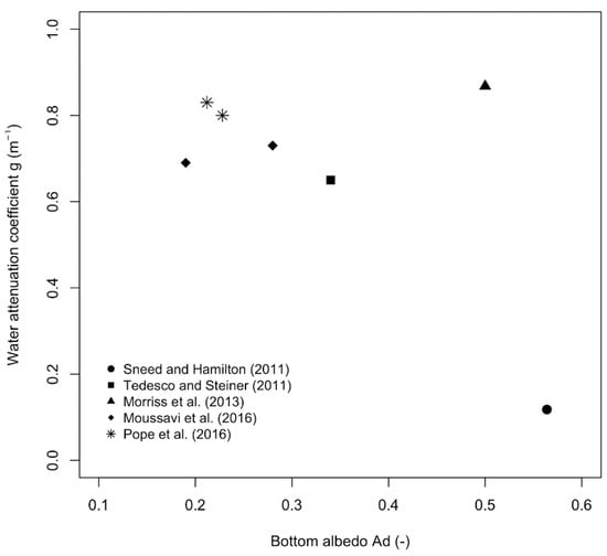
Figure 1.
Comparison of the water attenuation coefficients with the lake albedo values from various published studies. Symbols represent different publications [14,24,26,42,47].
In parallel to the above-mentioned SGL depth retrieval physical method, Lee et al. [48] developed a hyperspectral remote-sensing reflectance model for shallow waters, deriving bottom depth. Albedo intensity is allowed to change spatially. The model (Lee et al. [48]) derives simultaneously bottom depths, albedo, and the water optical properties (chlorophyll-a and gelbstoff for instance). The SPM is, however, not a parameter of the model. The model is designed for sea and ocean waters and not supraglacial lakes.
Williamson et al. [33] and Pope et al. [14] recall that the assumptions of the SGL physically based model are also potential weaknesses, which remain unquantified in the literature. The objective of this study is to quantify the effect of suspended particulate matter (SPM) on the SGL depth retrieval from optical data. We assume the SPM is an important property of the water, which influences the interaction of electromagnetic radiation with the medium. This effect is well known and scientifically studied for non-SGL waters and described by several publications [49,50]. The effect of SPM is not modelled by the Philpot [41] physical model used for the SGL depth retrieval; it may, however, potentially impose one of the uncertainties. We hypothesize that non-zero SPM concentration may negatively influence the model performance, given the increasing absorption of electromagnetic radiation with increasing SPM concentration.
The study presents spectral curves of the clear and SPM-affected supraglacial water for the first time. The spectral curves are measured in the visible and near-infrared electromagnetic spectrum ranging from 350 nm to 900 nm, which we refer to as optical data. Next, we present the results of in-situ experimental data based on concurrent hyper-spectral and bathymetric lake depth measurements. We address the unquantified assumption of the physical model, namely, that which pertains to suspended particulate matter (SPM) in the lake water. The objective is divided into several partial tasks. We first evaluate the SGL depth retrieval method from optical hyperspectral records under the presence of SPM using the empirical model based on concurrent hyperspectral and bathymetric lake depth measurements. Subsequently, we apply the SGL physically based model and update the attenuation coefficient of the model to improve its performance for the given SPM concentration of SGL water measured in-situ. Finally, we quantify the effect of maximum detectable lake depth for water with non-zero SPM.
2. Data and Methods
2.1. Characteristics of the Study Area
For our field experiment, we chose a lake on the Glacier de la Plaine Morte in the Bernese Alps in Switzerland (Figure 2). This lake (Lac des Faverges) is an ice-marginal lake; nevertheless, the bottom of the northern part of the lake is created by a glacier, making it suitable for our experiment as an SGL. A considerable part of the Glacier de la Morte is impermeable to water flow. Therefore, meltwater accumulates in surface streams [51]. According to Hählen [52], the lake has a considerable water volume of about 1.5 Mm3, and growth is expected. Lac des Faverges, as well as another two smaller lakes on the margin of the Glacier de la Morte, is formed at the border of a glacier and impermeable sediments, making it potentially unstable. Between 2011 and 2013, some of the lakes were subject to subglacial drainage [52]. Lac de Faverges is refilled annually, and meltwater accumulates in the lake basin. After reaching the maximum level of 2752 m above sea level, the lake water is drained through a superficial channel in the moraine deposit towards the Tièche basin [51]. Lindner et al. [53] described the typical fractures on the Glacier Plaine de la Morte on a centimeter or decimeter scale.
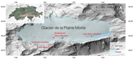
Figure 2.
Glacier de la Plaine Morte and its location within Switzerland (upper left inset). Coordinates in latitude and longitude. The location of the in-situ data collection is marked with red triangles. (Background maps: Swiss Open Data).
2.2. Collection of Experimental Data
2.2.1. Spectral Data
We collected 158 field spectra and depth measurements from Lac des Faverges and 30 additional spectra from a small pond with limited depth of 50 cm, both on the Glacier de la Plaine Morte. The spectral data were collected using an ASD FieldSpec® 4 (ASD Inc., Boulder, USA) high-resolution spectroradiometer instrument in the spectral range of visible (VIS) to shortwave-infrared wavelengths. The instrument acquired a continuous spectrum of λ = 350 to 2500 nm.
The spectroradiometer was calibrated using a white reference panel (Spectralon®—Labsphere Inc., North Sutton, NH, USA, diffuse reflectance material), the same calibration panel as for instance used by Tedesco and Steiner [26] as well as Moussavi et al. [24] and Pope et al. [14]. The calibration was checked before and after the data collection. Conversion of the collected FieldSpec® (ASD Inc., Boulder, CO, USA) DN values to reflectance followed the standard procedure using the white reference data. Each collected lake spectra consisted of 50 replications, which were averaged before conversion to reflectance. Due to a low signal of water reflectance at wavelengths longer than λ = 900 nm, the analysis focused on Rlake calculated in a range between 350 and 900 nm. Furthermore, an ASD contact probe was used to measure the spectra of the rock samples (limestone and clayey shale) collected from the sample locations, and sediment from the edge of the glacier.
2.2.2. Bathymetric Data
The RiverSurveyor system (SonTek) was used for in-situ depth measurements of the SGL. The system includes a 0.5 MHz echo-sounder with integrated GPS and a separate RTK Base Station. The echo-sounder was situated on the hydroboard together with the ASD FieldSpec® (ASD Inc., Boulder, CO, USA) 4 spectroradiometer. The measured depths were collected with an accuracy of 1 cm. Prior to the measurement, the accuracy of the echolot was validated using a manual depth measurement of up to 12 m. The comparison of the manual and echolot data revealed very high correspondence (Mean Absolute Error MAE = 0.292 m, RMSE = 0.353 m, coefficient of determination R2 = 0.999). Low water depths (less than 0.3 m) were measured using a hand meter.
2.2.3. Water Laboratory Analysis
At the time of bathymetric profiling (at the same place as the spectrum measurements), two water samples (1.5 L) were taken for laboratory gravimetric determination of the suspended particle concentration [54]. PRAGOPOR 4 membrane filters with a diameter of 50 mm and a pore size of 0.85 µm were used to filter the water samples taken. The empty filter weight was 0.064 g. The dried filter (105 °C) was weighed after filtration on KERN PCB precision scales. Water transparency was measured using a 30 cm diameter Secchi disc, and the physical parameters of the lake water were measured using a YSI 6920 multiparametric probe (temperature and conductance sensors). The default value (0.65) for conversion of specific conductance in μs/cm to total dissolved solids (TDS) in mg/L was used. We are aware that it is only useful for the gross estimate of the TDS [55].
2.3. Methods
2.3.1. Partial Least Squares Regression (PLSR)
In the first analysis, we performed the empirically based modelling using the PLSR multivariate regression method to estimate the SGL depth, given the fact we collected full continuous spectral data. The matrix of predictors (spectra) has more variables than the observations and multicollinearity among the spectra exists. For every measured lake depth, we used 551 spectral values. The PLSR method is different from those used in the other studies. The advantage is the loading values calculated by PLSR, which provide information on the influence of the spectra on the model.
The PLS package in R [56], was employed to model the relationship between the collected lake depth and the spectra records. The original spectral values from the FieldSpec® 4 (ASD Inc., Boulder, USA) instrument were converted into spectral reflectance and limited to a spectral range of λ = 350 nm to 900 nm (spectral values in a longer wavelength reached zero values) prior to PLSR analysis.
The PLSR model was trained with the collected in-situ data set, whereby a maximum of 10 components were used to calibrate the model. The model was cross-validated using the leave-one-out (LOO) segments while evaluating the root mean square error of predictions (RMSEP). The RMSEP was used to select the “best” model against the number of factors. To evaluate the model performance, we plotted the RMSEPs against the number of components in the model. The relative change of RMSEP with the number of factors compared to the minimum RMSEP was used to choose the number of components in the model. The coefficient of multiple determinations R2 was also assessed as the quality parameter of the model, but only as a secondary parameter. The first two PLSR factor loadings, considered to be indicators of the correlation between the spectra and the water depth, were also plotted for a qualitative interpretation.
Alongside the above-described model cross-validation during the training phase, we initially split the original full data set into train (calibration) and test (validation) subsets to evaluate the model performance on a set of samples that were not used in the empirical model construction. We applied stratified sampling while selecting 70% for mode training and 30% for model testing.
2.3.2. Physical Model
Philpot [41] describes a simple radiative transfer model for optically shallow waters of the general form:
where Ld is the radiance observed on the remote (proximal) detector, Lb is a radiance term, which is sensitive to bottom reflectance, g is a two-way attenuation coefficient of the water, z is the depth of the water column, and Lw is the radiance observed over optically deep water.
Ld = Lb exp(−gz) + Lw,
Solving the radiative transfer model, Philpot [41] provides a logarithmic form with the approximation of the lake depth z in meters as:
where, Rlake is the reflectance measured from the lake in the location of interest.
z = [ln(Ad − R∞) − ln(Rlake − R∞)]/g,
The two-way attenuation coefficient g accounts for losses in both the upward and downward travel through the water column in m−1. Philpot [41] relates the g parameter to the diffuse attenuation of the downwelling light (kd), the beam absorption coefficient, and the distribution factor for upwelling irradiance Du:
g ~ kd + a Du.
All the parameters, except the depth, are wavelength dependent. The two-way attenuation coefficient g depends on the absorption coefficient and the backscattering coefficients, which are modified by the concentration and type of SPM. Sneed and Hamilton [10] measured the total suspended solids to be 0.74 mg/L and 0.20 mg/L in samples of melt pond water taken from the Helheim glacier, east Greenland. However, the respective g coefficients used in the study were not presented; hence, the effect was not quantified. All other authors assume no or minimal influence of SPM. To apply the physically based model, the Ad, R∞, and g parameters must be determined before the depth estimation.
We ran the water depth retrieval with a physically based model as provided in Equation (2). The model is applied to evaluate the effect of the SPM on the model with physical basis. The published studies on SGL depth retrieval with physically based single-band models used various bands, typically green, red, or NIR. Early studies, for instance Georgiou et al. [19], focused more on the green band, which corresponds to λ = 525–605 nm using the Landsat-7 sensor, whereas later studies, for instance Sneed and Hamilton [42], focused more on the red band, which corresponds to λ = 630–690 nm using the Landsat-7 sensor. Pope et al. [14] concluded that the optimal SGL depth retrieval may be achieved by a physically based single-band model applied to Landsat-8 OLI red and panchromatic bands and subsequently averaging the retrieval results.
To apply the single-band physical model, we decided to use the model parameters and recommendations after Pope et al. [14] (see Table 1) for Landsat-8. Pope et al. [14] assume that “it is possible to apply locally calibrated coefficients to broader areas”. The physical model will better generalize compared to the empirical model. However, we will also consider the local condition of the water in the Lac des Faverges, i.e., the presence of SPM, which directly affects the water attenuation. Hence, we re-calibrate the g parameter. Furthermore, we assume that the other two parameters are plausible values of the model for Landsat-8 red band and independent of the water properties as such the presence of the SPM.
Firstly, we convolved the original in-situ FieldSpec® 4 (ASD Inc., Boulder, USA) records to the Landsat-8 OLI red band according to the spectral response function in the range of λ = 630 to 680 nm (Barsi et al. [57]). The coefficient of attenuation g was initially set to 0.80 m−1 according to Pope et al. [14] (based on in-situ regressed data). The albedo of the lake bottom Ad was set to 0.228, and the irradiance reflectance of optically deep-water R∞ was set to a value of 0.0375. Given the fact that there was a higher concentration of SPM in the lake water, we re-fitted the g parameter to reflect the local conditions. The g parameter was fitted as a free parameter in the physical model (Equation (2)) using the least squares method from the R-package. This parametrization provided us with a way to quantify the change of the water attenuation in the event of the presence of SPM in the water.
3. Results
3.1. Supraglacial Lake Water Spectral Signatures
The spectral signatures of the SGL water at Lac des Faverges with changing water depth (Figure 3) are presented in Figure 4a; the glacier ice, moraine sediment, and rock spectra are presented in Figure 4b.
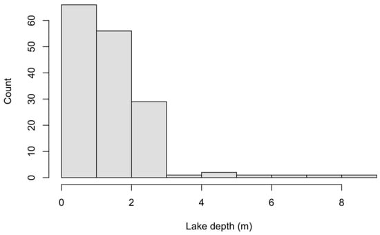
Figure 3.
Histogram of the measured lake depths at Lac des Faverges.
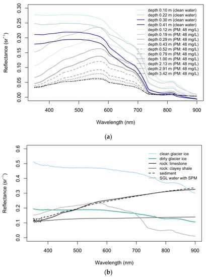
Figure 4.
Supraglacial lake water spectra (a), ice, moraine sediment, and water spectra (b) at Glacier de la Plaine Morte.
The blue lines in Figure 4a represent the measured clean water at a small pond nearby the lake, limited to 0.4 m, while the black/grey lines represent the data measured from Lac des Faverges, which are affected by the presence of SPM. We plotted the spectra only up to 900 nm since the water reflectance in the higher wavelengths tends towards zero.
The in-situ measured water depth ranged from 0.12 to 8.62 m as presented in Figure 3. The main data set collected in the field, however, ranged up to approximately 3 m in depth. We present the spectral curves of the water with SPM (Figure 4a) ranging from 0.12 m to 3.42 m in depth, while the spectra of 2.91 m and 3.42 m in depth overlap each other. We did not plot the additional spectra of the higher depths up to the measured 8.62 m as there is no significant spectral difference. The saturation effect due to the presence of SPM is evident in the spectral curves. The concentration of SPM measured in Lac des Faverges’ water on 16 July 2019, was 48 mg/L. The transparency of the water in the lake, measured using a Secchi disc, was determined to be 0.7 m. Other physical quantities measured in-situ in the vertical profile were temperature, conductivity, and the total amount of solutes. Figure 5 shows that the lake was not vertically stratified at the time of measurement, satisfying the vertical homogeneity assumption.
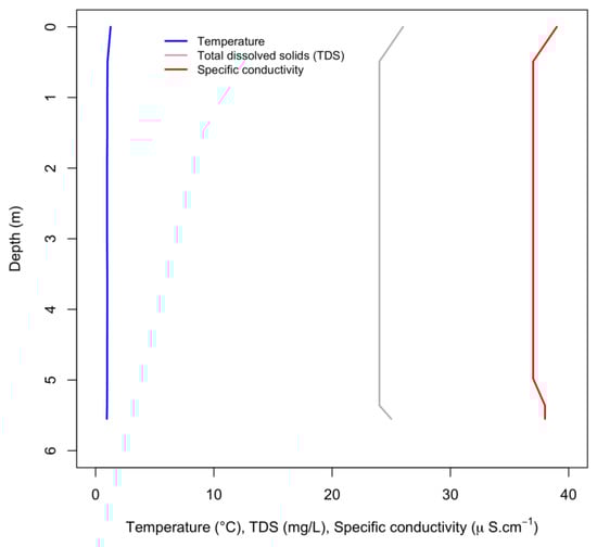
Figure 5.
Water temperature, dissolved solids and specific conductivity of total dissolved solids (TDS) in Lac des Faverges at the time of SGL measurements.
Figure 4a illustrates that the spectral reflectance of the SGL water decreases with increasing water depth of the lake. It is noticeable that the difference between the clear water spectra and the water affected by SPM becomes minimal from around 680 nm. The maximum difference between the lake water spectra with suspended SPM and those spectra at which we assume the saturation effects begin (2.91 m in depth) was then calculated as the median at the 576 nm spectra, which corresponds to the green band of the Landsat sensor. This spectral band theoretically provides the highest range for the model, either empirical or physical.
Furthermore, we present the spectral curves of the clean glacier and glacier ice affected by the deposit particles, the spectral curves of the rock near the glacier (limestone and clayey shale), and its sediment collected at the edge of the Glacier de la Plaine Morte (Figure 4b). Both glacier spectra are monotonously decreasing with an increasing wavelength up to 900 nm. The difference is in the absolute values of the reflectance modified by the presence of impurities on the glacier surface. Pure ice is very weakly absorptive in the VIS spectral region. The observed absorption in the VIS is the tail of NIR vibrational absorptions [58]. Therefore, the absorption increases with increasing wavelength from blue to red. The rock and sediment spectra exhibit an increase, on the other hand, with the wavelength. The spectral effect of the SPM in the lake water corresponds to the sediment spectra up to 700 nm.
3.2. SGL Depth Retrieval by the PLSR Model
We constructed the first empirical PLSR model (abbreviated as 1) from all the collected data from Lac des Faverges (water with SPM) up to 8.62 m, even though the saturation effect is well visible from the plotted spectra (Figure 4a). Additionally, we constructed a model (abbreviated as 1b) from the spectra collected from the small pond (clean water), limited to the depth of about 50 cm. The models were cross-validated using the “leave-one-out” method. The RMSEP indicator proved that the PLSR model 1a with the first five components provides the best option. The lake depth values predicted against the in-situ measured data revealed that the model does not explain the variation for depths higher than approximately 3.0 m (Figure 6), which confirms the saturation effect visible in the plotted spectra (Figure 4a). Additionally, it documents the effect of the SPM in the water on empirical modelling of the SGL depth, albeit to the limited depth of the clean water. The model 1a shows not only the saturation effect but also the much higher dispersion of the points from the 1:1 line (Figure 6). Performance of the models is summarized in Table 2. The model 1b was only cross validated; a testing subset was not created due to the limited number of records.
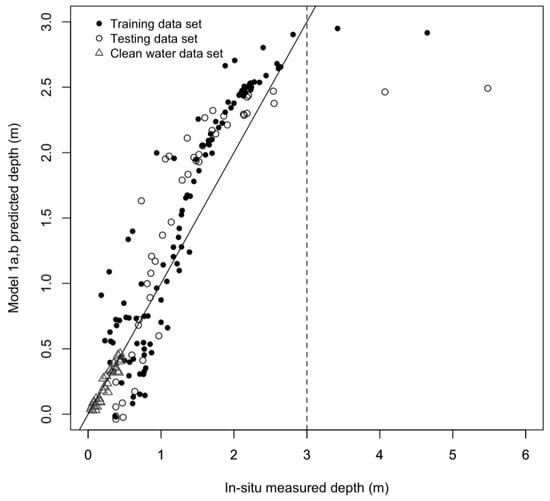
Figure 6.
Scatter plot of observed SGL depth against the cross-validated PLSR predicted for the full datasets.
Table 2.
PLSR model quality indicators.
In the subsequent analysis, we constructed a second PLSR model (abbreviated as model 2) limiting the lake depth readings to 3.0 m only, to evaluate the model performance in this range and to avoid the effect of the saturation caused by SPM. The range of the depth in the training (calibration) data set is 0.1 to 2.91 m and the range in the testing (validation) data set is 0.34 to 2.55 m.
The RMSEP indicator showed local minima at seven components (Figure 7), while the first two components explained most of the variation.
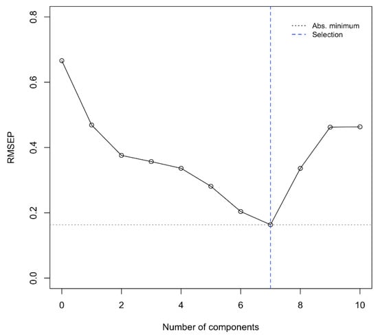
Figure 7.
The PLSR model 2 cross-validated root mean square error of prediction (RMSEP) against the number of factors.
The first component explained 98.1% of the variation, and the second component contributed 1.6% (Figure 8). The quality indicators of models 1 and 2 are presented in Table 2. The resulting model 2 scatter plot of the observed SGL depth against the cross-validated PLSR predicted is depicted in Figure 9.
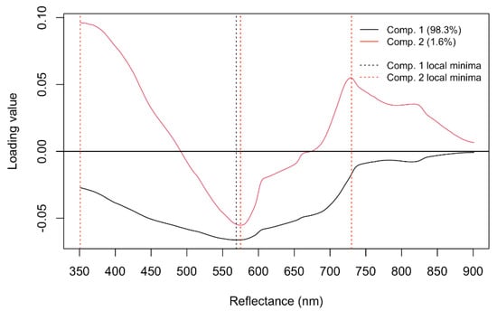
Figure 8.
The two PLSR model 2 factor loading weight vectors with local maxima (vertical lines).
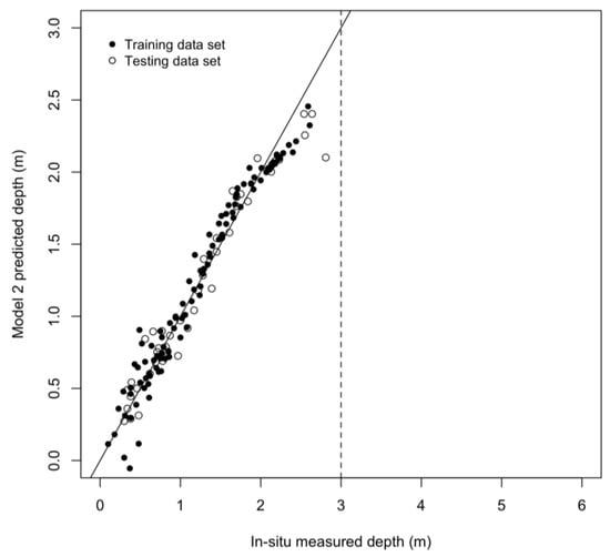
Figure 9.
Scatter plot of observed SGL depth against the cross-validated PLSR predicted for the limited datasets.
3.3. SGL Depth Retrieval by the Physically Based Model
In the analysis with the physically based model, we initially ran the model (1) with parameterization as estimated by Pope et al. [14] for the Landsat-8 sensor, red band. To apply the single-band model, we convolved the continuous FieldSpec® 4 (ASD Inc., Boulder, USA) records based on the relative spectral response curve for Landsat-8 [55] (Figure 10). Although the SGL water spectral values in the range of the broad Landsat-8 red band are monotonous and the effect of convolution is minimal, we applied this step for full consistency, while using the parameterization of the model for the Landsat-8 band.
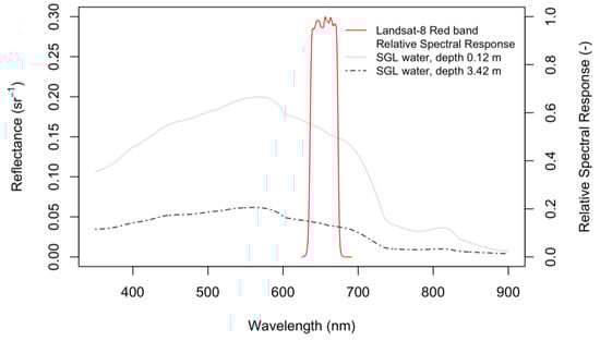
Figure 10.
Landsat-8 red band relative spectral response curve and samples of SGL water.
The physical model 1 predictions against our in-situ measured water lake depths at Lac des Faverges (SPM = 48 mg/L) are presented in Figure 11 (open triangles).The predicted lake depth values are highly overestimated given the fact that we used the g parameter (attenuation coefficient), which was regressed for water without the presence of SPM. The model 1 quality metrics (RMSE and R2) are presented in Table 3. In order to quantify the effect of SPM (48 mg/L) in the lake water on the change of the water attenuation, we re-fitted the physical model with g as a free parameter. The original attenuation coefficient g was 0.8 m−1, while the newly fitted g equals 2.42 m−1. We fitted physical model 2 to the training data set (Figure 11, full dot) limited to a plausible depth of 3.0 m as determined in the previous analysis, since the water spectra became saturated at greater depths given the presence of SPM. The model 2 quality metrics are presented in Table 3.
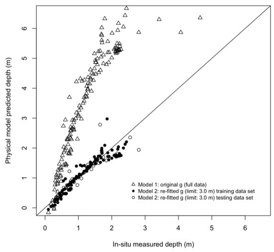
Figure 11.
Scatter plot of the physically based model prediction against the in-situ measurements.
Table 3.
SGL physical model quality metrics.
4. Discussion
The resulting empirical PLSR model (2), and physically-based model (2) both proved there is still a good relationship between the water reflectance spectra and the supraglacial lake depth under the constraint of SPM in the water (48 mg/L in our case). However, applicability of the depth–reflectance relationships was limited to a depth of approximately 3 m given the constraint. The physical principle holds true within this limit. We compared these results to those of previous studies where in-situ or other independent reference measurements were taken, although they used different optical sensors. Georgiou et al. [19] calculated the RMSE between the ASTER image estimated depth and Lidar depths to be 0.7 m using a physically based model, while the RMSE dropped to 0.3 m in cloud-free areas. The depths across the Lidar transect varied between 0 and 4 m. Tedesco and Steiner [26] reported RMSE of 0.59 m (R2 = 0.84) compared to in-situ (GPS/sonar) measurements, and RMSE of 0.45 m (R2 = 0.85) for a re-fitted diffuse attenuation coefficient while using the Landsat-7 green band. The maximum measured depth was 4.5 m. Pope et al. [14] provided statistical quality indicators of their physically based model using the Tedesco and Steiner [26] and Tedesco et al. [26] in-situ data (2226 unique sample points). Their results accounted for RMSE of 0.28 m (R2 = 0.96) when using the Landsat-8 OLI red band as the best result. The maximum in-situ lake depth measured was 5 m in their study. Our reported results of the PLSR model 2 showed RMSE = 0.163 m (R2 = 0.93) for PLSR training and RMSE = 0.186 m (R2 = 0.93) for PLSR model testing (Table 2). The physically based model 2 showed RMSE = 0.243 m (R2 = 0.86) (Table 3), which is in line with the previous studies, albeit limited by the depth. The empirical model performed better than the physically based model even after the update of the g parameter. Moreover, the empirical model based on clean water performed better than the model constructed from SPM affected water data.
The depth limit was estimated to be around 3 m in our study, beyond which the increase in depth cannot be modelled due to the SPM concentration 48 mg/L. However, when revising the scatterplot of the PLSR model 1 (Figure 6), as well as the scatterplot of the physical model 2 (Figure 11), although the data were limited to the depth of 3.0 m, the flattening effect due to the presence of SPM starts earlier, at around 2 m. The SGL water spectra of 2.13 m and 2.91 m in depth (Figure 4a) are close to each other, leaving very little space for modelling the variability of about 0.8 m difference.
Given the above discussed limits of lake water depth retrieval under the presence of SPM in the water, we also analysed the maximum detectable depth based on the general expression by Philpot [41] for bathymetric mapping with passive multispectral imagery. Philpot [41] states: “the maximum detectable depth may be defined as the depth at which the difference between the observed radiance (Ld) and that for an optically deep-water mass (Lw) is equivalent to one digital count (ΔLDN = Ld − Lw)”. The maximum detectable depth is expressed as:
zmax = −ln(ΔLDN/Lb)/g.
Philpot [41] describes the maximum detectable depth using several LDN/Lb ratios. Selecting the ratio value of 0.001 from the Philpot [41] publication, Figure 12 shows the change in the maximum detectable depth for various water attenuation coefficients. The detectable maximal depth increases with a decrease in the effective attenuation coefficient g. In a case where the water attenuation coefficient g = 2.42 m−1 (re-fitted value for lake water with SPM concentration of 48 mg/L at Lac des Faverges), the maximum detectable depth is 2.9 m. This corresponds to our previous findings described in Section 3.1, Section 3.2 and Section 3.3. The maximum detectable depth would increase up to 8.91 m in the case of an attenuation coefficient g = 0.8 m−1, using the value of g estimated by Pope et al. [14] from in-situ data collected from Greenland, assuming there was no dissolved or suspended SPM in the lake water. This illustrates the importance of the attenuation coefficient parameter in the model.
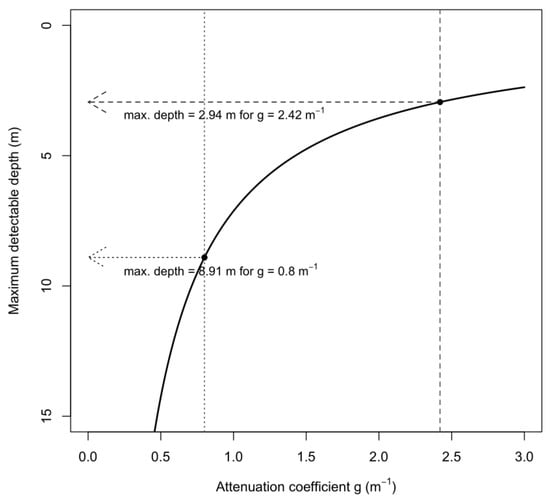
Figure 12.
Maximum detectable depth relative to the water attenuation coefficient.
Another factor to consider in the context of the detectable lake depth is the sensor used. In our study, we used the FieldSpec® 4 (ASD Inc., Boulder, USA) in-situ instrument close to the water surface (about 0.15 m); hence, our measurements excluded atmospheric path radiance effects, which are present in the satellite earth observation data even though atmospheric corrections are applied.
The PLSR empirical model applied to the full hyperspectral data did not only model the relationship between the variables but also provided the loadings per continuous spectra. The PLSR loading values revealed the significance of the 569 and 575 nm bands for the model. Our findings, using full hyperspectral data, suggest using green bands. Pope et al. [14] concluded that longer wavelengths (e.g., the red band) may generally provide more accurate lake depths, explaining that there is a larger change in net reflectance for red wavelengths than shorter wavelengths. This contrasts with our findings, where the largest change was calculated to be in the 576 nm spectra (green band), albeit for water affected by SPM. Tedesco and Steiner [26] state that the red band is less sensitive to changing albedo values in comparison with the green band. Moussavi et al. [24] obtained more accurate results when using green and red bands together for shallow lake areas.
The physically based model was developed as a single-band model assuming there is no present or little suspended or dissolved particulate matter, which would affect the water leaving radiance. Sneed and Hamilton [42] measured SPM of 0.74 and 0.2 mg/L in eastern Greenland. Sneed and Hamilton [42] concluded that, based on three years of melt water analysis, they are confident that dissolved or SPM plays a minor role in accurately determining meltwater depth in Greenland. However, they also suggested taking a larger sample set from different regions of Greenland. Other authors assumed no influence of SPM in the water.
5. Conclusions
In this study, we assessed the effect of SPM in SGL water on lake depth retrieval. We collected in-situ measurements of hyperspectral and lake depth observations over an SGL to 8 m in depth. These measurements allowed us to construct both empirical (PLSR) and physically based models. Our lake water measurements satisfied most of the inherent assumptions of the physically based model, i.e., the optical properties of the water were vertically homogeneous, the lake surface was not disturbed by wind, and we did not identify any ice bottom inhomogeneity. However, there was a non-minimal concentration of SPM in the water.
The influence of the suspended particles in the lake water is evident in the lake spectral curves. There is a profound absorption effect in the shorter wavelength up to about 600 nm. However, the lake spectra still exhibit a change with lake depth. The maximum difference between lake water spectra and changing depth was calculated to be 576 nm.
The modelling results show that there is still a good relationship between SGL water spectra and the lake depth in the presence of 48 mg/L of SPM; however, it is limited by the maximum detectable depth of approximately 3 m. The effect of the SPM in water affected the depth–reflectance relationships from approximately 2 m in depth; however, the model’s quality parameters confirmed the validity of the results up to 3 m. The RMSE values of 0.163 and 0.243 m of our empirical and physically based models, respectively, are within the range of previous published studies, or are even lower. The indicated depth limit was also confirmed by constructing the physically based model as well as using the general expression for the maximum detectable depth from Philpot [45]. However, the physically based model attenuation coefficient g required re-fitting for the lake conditions. The value of g increased from 0.8 m−1 (Pope et al. [14]) to 2.42 m−1 due to the presence of SPM with a concentration of 48 mg/L.
The empirical model performed better compared to the physically based model; it fitted better the in-situ measurements, while the physically based model is considered as more generic and has better potential of transferability. However, the transferability would be limited to the situations of the same water properties such as, for instance, the SPM concentration. The physically based model does not model varying concentrations of the water properties.
The physically based remote-sensing reflectance model for SGL depth retrieval might be improved in the future by allowing, for instance, the simultaneous derivation of bottom depths, albedo, and possible varying water optical properties, like the model developed by Lee et al. [48].
The physically based model for bathymetric mapping from optical data was originally designed with several assumptions, one of which was no presence of SPM in the water. This study demonstrated the effect of non-zero SPM in the water on the model performance. We conclude that the original hypothesis that non-zero SPM concentration may negatively influence the model performance is true. Moreover, we demonstrated how it limits the maximum detectable depth of SGL from optical data.
Author Contributions
Conceptualization, L.B. and V.V.; methodology, L.B. and M.Š.; resources, L.B., V.V., M.Š. and T.K., formal analysis, L.B.; writing—original draft preparation, L.B.; editing, V.V., M.Š. and T.K.; visualization, L.B.; funding acquisition, V.V. All authors have read and agreed to the published version of the manuscript.
Funding
This research was funded by the 4EU+ project, grant number: 4EU+/21/F4/21 and partly by the Grant Agency of Charles University (Project GAUK No. 1164320).
Acknowledgments
Computational resources were supplied by the project “e-Infrastruktura CZ” (e-INFRA CZ LM2018140) supported by the Ministry of Education, Youth and Sports of the Czech Republic.
Conflicts of Interest
The authors declare no conflict of interest.
References
- Hutchinson, G.E. A Treatise on Limnology. In Geography, Physics, and Chemistry; John Wiley & Sons, Inc.: New York, NY, USA, 1957; Volume 1. [Google Scholar]
- Gardelle, J.; Arnaud, Y.; Berthier, E. Contrasted evolution of glacial lakes along the Hindu Kush Himalaya mountain range between 1990 and 2009. Glob. Planet. Chang. 2011, 75, 47–55. [Google Scholar] [CrossRef]
- Miles, E.S.; Steiner, J.; Willis, I.; Buri, P.; Immerzeel, W.W.; Chesnokova, A.; Pellicciotti, F. Pond Dynamics and Supraglacial-Englacial Connectivity on Debris-Covered Lirung Glacier, Nepal. Front. Earth Sci. 2017, 5, 69. [Google Scholar] [CrossRef]
- Baťka, J. Factors of formation and development of supraglacial lakes and their quantification: A review. AUC Geogr. 2016, 51, 205–216. [Google Scholar] [CrossRef]
- Benn, D.I.; Bolch, T.; Hands, K.; Gulley, J.; Luckman, A.; Nicholson, L.I.; Quincey, D.J.; Thompson, S.; Toumi, R.; Wiseman, S. Response of debris-covered glaciers in the Mount Everest region to recent warming, and implications for outburst flood hazards. Earth-Sci. Rev. 2012, 114, 156–174. [Google Scholar] [CrossRef]
- Sakai, A. Glacial Lakes in the Himalayas: A Review on Formation and Expansion Processes. Glob. Environ. Res. 2012, 16, 23–30. [Google Scholar]
- Liu, Q.; Mayer, C.; Liu, S. Distribution and recent variations of supraglacial lakes on detritic-type glaciers in the Khan Tengri-Tomur Mountains, Central Asia. Cryosphere Discuss. 2013, 7, 4545–4584. [Google Scholar] [CrossRef]
- Emmer, A.; Loarte, E.; Klimeš, J.; Vilímek, V. Recent evolution and degradation of the bent Jatunraju glacier (Cordillera Blanca, Peru). Geomorphology 2015, 228, 345–355. [Google Scholar] [CrossRef]
- Vilímek, V.; Klimeš, J.; Červená, L. Glacier-related landforms and glacial lakes in Huascarán National Park, Peru. J. Maps 2016, 12, 193–202. [Google Scholar] [CrossRef]
- Sneed, W.A.; Hamilton, G.S. Evolution of melt pond volume on the surface of the Greenland Ice Sheet. Geophys. Res. Lett. 2007, 34, L03501. [Google Scholar] [CrossRef]
- Das, S.B.; Joughin, I.; Behn, M.D.; Howat, I.M.; King, M.A.; Lizarralde, D.; Bhatia, M.P. Fracture propagation to the base of the Greenland ice sheet during supraglacial lake drainage. Science 2008, 320, 778–781. [Google Scholar] [CrossRef]
- Langley, E.S.; Leeson, A.A.; Stokes, C.R.; Jamieson, S.S.R. Seasonal evolution of supraglacial lakes on an East Antarctic outlet glacier. Geophys. Res. Lett. 2016, 43, 8563–8571. [Google Scholar] [CrossRef]
- Banwell, A.F.; Caballero, M.; Arnold, N.S.; Glasser, N.F.; Cathles, L.M.; MacAyeal, D.R. Supraglacial lakes on the Larsen B ice shelf, Antarctica, and at Paakitsoq, West Greenland: A comparative study. Ann. Glaciol. 2014, 55, 1–8. [Google Scholar] [CrossRef]
- Pope, A.; Scambos, T.A.; Moussavi, M.; Tedesco, M.; Willis, M.; Shean, D.; Grigsby, S. Estimating supraglacial lake depth in West Greenland using Landsat 8 and comparison with other multispectral methods. Cryosphere 2016, 10, 15–27. [Google Scholar] [CrossRef]
- Benn, D.I.; Wiseman, S.; Warren, C.R. Rapid growth of a supraglacial lake, Ngozumpa Glacier, Khumbu Himal, Nepal. In Debris-Covered Glaciers, Proceedings of the Seattle Workshop, Seattle, WA, USA, 13–15 September 2000; Nakawo, M., Raymond, C.F., Fountain, A., Eds.; IAHS Press: Wallingford, UK, 2000; Volume 264, pp. 177–185. [Google Scholar]
- Everett, A.; Murray, T.; Selmes, N.; Rutt, I.C.; Luckman, A.; James, T.D.; Reeve, D.E. Annual down-glacier drainage of lakes and water-filled crevasses at Helheim Glacier, southeast Greenland. J. Geophys. Res. Earth Surf. 2016, 121, 1819–1833. [Google Scholar] [CrossRef]
- McMillan, M.; Nienow, P.; Shepherd, A.; Benham, T.; Sole, A. Seasonal evolution of supra-glacial lakes on the Greenland Ice Sheet. Earth Planet. Sci. Lett. 2007, 262, 484–492. [Google Scholar] [CrossRef]
- Leeson, A.A.; Shepherd, A.; Sundal, A.V.; Johansson, A.M.; Selmes, N.; Briggs, K.; Fettweis, X. A comparison of supraglacial lake observations derived from MODIS imagery at the western margin of the Greenland ice sheet. J. Glaciol. 2013, 59, 1179–1188. [Google Scholar] [CrossRef]
- Georgiou, S.; Shepherd, A.; Mcmillan, M.; Nienow, P. Seasonal evolution of supraglacial lake volume from aster imagery. Ann. Glaciol. 2009, 50, 95–100. [Google Scholar] [CrossRef]
- Huss, M.; Hock, R. Global-scale hydrological response to future glacier mass loss. Nat. Clim. Chang. 2018, 8, 135–140. [Google Scholar] [CrossRef]
- Box, J.; Ski, K. Remote sounding of Greenland supraglacial melt lakes: Implications for subglacial hydraulics. J. Glaciol. 2007, 53, 257–265. [Google Scholar] [CrossRef]
- Sundal, A.V.; Shepherd, A.; Nienow, P.; Hanna, E.; Palmer, S.; Huybrechts, P. Evolution of supra-glacial lakes across the Greenland Ice Sheet. Remote Sens. Environ. 2009, 113, 2164–2171. [Google Scholar] [CrossRef]
- Ignéczi, Á.; Sole, A.J.; Livingstone, S.J.; Leeson, A.A.; Fettweis, X.; Selmes, N.; Briggs, K. Northeast sector of the Greenland Ice Sheet to undergo the greatest inland expansion of supraglacial lakes during the 21st century. Geophys. Res. Lett. 2016, 43, 9729–9738. [Google Scholar] [CrossRef]
- Moussavi, M.S.; Abdalati, W.; Pope, A.; Scambos, T.; Tedesco, M.; MacFerrin, M.; Grigsby, S. Derivation and validation of supraglacial lake volumes on the Greenland Ice Sheet from high-resolution satellite imagery. Remote Sens. Environ. 2016, 183, 294–303. [Google Scholar] [CrossRef]
- Miles, K.E.; Willis, I.C.; Benedek, C.L.; Williamson, A.G.; Tedesco, M. Toward monitoring surface and subsurface lakes on the Greenland ice sheet using sentinel-1 SAR and landsat-8 OLI imagery. Front. Earth Sci. 2017, 5, 58. [Google Scholar] [CrossRef]
- Tedesco, M.; Steiner, N. In-situ multispectral and bathymetric measurements over a supraglacial lake in western Greenland using a remotely controlled watercraft. Cryosphere 2011, 5, 445–452. [Google Scholar] [CrossRef]
- Liang, Y.-L.; Colgan, W.; Lv, Q.; Steffen, K.; Abdalati, W.; Stroeve, J.; Gallaher, D.; Bayou, N. A decadal investigation of supraglacial lakes in West Greenland using a fully automatic detection and tracking algorithm. Remote Sens. Environ. 2012, 123, 127–138. [Google Scholar] [CrossRef]
- Shugar, D.H.; Burr, A.; Haritashya, U.K.; Kargel, J.S.; Watson, C.S.; Kennedy, M.C.; Bevington, A.R.; Betts, R.A.; Harrison, S.; Strattman, K. Rapid worldwide growth of glacial lakes since 1990. Nat. Clim. Chang. 2020, 10, 939–945. [Google Scholar] [CrossRef]
- Baťka, J.; Vilímek, V.; Štefanová, E.; Cook, S.J.; Emmer, A. Glacial Lake Outburst Floods (GLOFs) in the Cordillera Huayhuash, Peru: Historic Events and Current Susceptibility. Water 2020, 12, 2664. [Google Scholar] [CrossRef]
- Schröder, L.; Neckel, N.; Zindler, R.; Humbert, A. Perennial Supraglacial Lakes in Northeast Greenland Observed by Polarimetric SAR. Remote Sens. 2020, 12, 2798. [Google Scholar] [CrossRef]
- Dirscherl, M.; Dietz, A.J.; Kneisel, C.; Kuenzer, C. Automated Mapping of Antarctic Supraglacial Lakes Using a Machine Learning Approach. Remote Sens. 2020, 12, 1203. [Google Scholar] [CrossRef]
- Moussavi, M.; Pope, A.; Halberstadt, A.R.W.; Trusel, L.D.; Cioffi, L.; Abdalati, W. Antarctic Supraglacial Lake Detection Using Landsat 8 and Sentinel-2 Imagery: Towards Continental Generation of Lake Volumes. Remote Sens. 2020, 12, 134. [Google Scholar] [CrossRef]
- Williamson, A.G.; Neil, S.A.; Alison, F.B.; Ian, C.; Willis, A. Fully Automated Supraglacial lake area and volume Tracking (“FAST”) algorithm: Development and application using MODIS imagery of West Greenland. Remote Sens. Environ. 2017, 196, 113–133. [Google Scholar] [CrossRef]
- Fitzpatrick, A.A.W.; Hubbard, A.L.; Box, J.E.; Quincey, D.J.; van As, D.; Mikkelsen, A.P.B.; Doyle, S.H.; Dow, C.F.; Hasholt, B.; Jones, G.A. A decade (2002−2012) of supraglacial lake volume estimates across Russell Glacier, West Greenland. Cryosphere 2014, 8, 107–121. [Google Scholar] [CrossRef]
- Williamson, A.G.; Banwell, A.F.; Willis, I.C.; Arnold, N.S. Dual-satellite (Sentinel-2 and Landsat 8) remote sensing of supraglacial lakes in Greenland. Cryosphere 2018, 12, 3045–3065. [Google Scholar] [CrossRef]
- König, M.; Birnbaum, G.; Oppelt, N. Mapping the Bathymetry of Melt Ponds on Arctic Sea Ice Using Hyperspectral Imagery. Remote Sens. 2020, 12, 2623. [Google Scholar] [CrossRef]
- Fricker, H.A.; Arndt, P.; Brunt, K.M.; Datta, R.T.; Fair, Z.; Jasinski, M.F.; Kingslake, J.; Magruder, L.A.; Moussavi, M.; Pope, A.; et al. ICESat-2 meltwater depth estimates: Application to surface melt on Amery Ice Shelf, East Antarctica. Geophys. Res. Lett. 2021, 48, e2020GL090550. [Google Scholar] [CrossRef]
- Datta, R.T.; Wouters, B. Supraglacial lake bathymetry automatically derived from ICESat-2 constraining lake depth estimates from multi-source satellite imagery. Cryosphere 2021, 15, 5115–5132. [Google Scholar] [CrossRef]
- Lai, W.; Lee, Z.; Wang, J.; Wang, Y.; Garcia, R.; Zhang, H. A Portable Algorithm to Retrieve Bottom Depth of Optically Shallow Waters from Top-Of-Atmosphere Measurements. J. Remote Sens. 2022, 2022, 16. [Google Scholar] [CrossRef]
- Studinger, M.; Manizade, S.S.; Linkswiler, M.A.; Yungel, J.K. High-resolution imaging of supraglacial hydro-logical features on the Greenland Ice Sheet with NASA’s Airborne Topographic Mapper (ATM) instrument suite. Cryosphere 2022, 16, 3649–3668. [Google Scholar] [CrossRef]
- Philpot, W.D. Bathymetric mapping with passive multispectral imagery. Appl. Opt. 1989, 28, 1569. [Google Scholar] [CrossRef]
- Sneed, W.A.; Hamilton, G.S. Validation of a method for determining the depth of glacial melt ponds using satellite imagery. Ann. Glaciol. 2011, 52, 15–22. [Google Scholar] [CrossRef]
- Mobley, C.D.; Sundman, L.K. Effects of optically shallow bottoms on upwelling radiances: Inhomogeneous and sloping bottoms. Limnol. Oceanogr. 2003, 48, 329–336. [Google Scholar] [CrossRef]
- Maritorena, S.; Morel, A.; Gentili, B. Diffuse reflectance of oceanic shallow waters: Influence of water depth and bottom albedo. Limnol. Ocean. 1994, 39, 1689–1703. [Google Scholar] [CrossRef]
- Pope, R.M.; Fry, E.S. Absorption spectrum 380-700 nm of pure water. II. Integrating cavity measurements. Appl. Opt. 1997, 36, 8710–8723. [Google Scholar] [CrossRef] [PubMed]
- Smith, R.C.; Baker, K.S. Optical properties of the clearest natural waters (200–800 nm). Appl. Opt. 1981, 20, 177. [Google Scholar] [CrossRef] [PubMed]
- Morriss, B.F.; Hawley, R.L.; Chipman, J.W.; Andrews, L.C.; Catania, G.A.; Hoffman, M.J.; Lüthi, M.P.; Neumann, T.A. A ten-year record of supraglacial lake evolution and rapid drainage in West Greenland using an automated processing algorithm for multispectral imagery. Cryosphere 2013, 7, 1869–1877. [Google Scholar] [CrossRef]
- Lee, Z.; Carder, K.L.; Mobley, C.D.; Steward, R.G.; Patch, J.S. Hyperspectral remote sensing for shallow waters. 2. Deriving bottom depths and water properties by optimization. Appl. Opt. 1999, 38, 3831–3843. [Google Scholar] [CrossRef]
- Gege, P. The water color simulator WASI: An integrating software tool for analysis and simulation of optical in situ spectra. Comput. Geosci. 2004, 30, 523–532. [Google Scholar] [CrossRef]
- Bernardo, N.; do Carmo, A.; Park, E.; Alcântara, E. Retrieval of Suspended Particulate Matter in Inland Waters with Widely Differing Optical Properties Using a Semi-Analytical Scheme. Remote Sens. 2019, 11, 2283. [Google Scholar] [CrossRef]
- Huss, M.; Voinesco, A.; Hoelzle, M. Implications of climate change on Glacier d e la Plain Morte, Switzerland. Geogr. Helv. 2013, 68, 227–237. [Google Scholar] [CrossRef]
- Hählen, N. Ausbruch Gletschersee Faverges, Oberingenieurkreis I, Civil Engineering Office of the Canton of Bern, Report, Gemeinde Lenk, 2012.
- Lindner, F.; Weemstra, C.; Walter, F.; Hadziioannou, C. Towards monitoring the englacial fracture state using virtual-reflector seismology. Geophys. J. Int. 2018, 214, 825–844. [Google Scholar] [CrossRef]
- Pfannkuche, J.; Schmidt, A. Determination of suspended particulate matter concentration from turbidity measurements: Particle size effects and calibration procedures. Hydrol. Process. 2003, 17, 1951–1963. [Google Scholar] [CrossRef]
- YSI Incorporated. Environmental Monitoring Systems Operations Manual; Yellow Springs: Ohio, OH, USA, 2002; p. 220. [Google Scholar]
- Mevik, B.-H.; Wehrens, R. The pls Package: Principal Component and Partial Least Squares Regression in R. J. Stat. Softw. 2007, 18, 1–23. [Google Scholar] [CrossRef]
- Barsi, J.A.; Lee, K.; Kvaran, G.; Markham, B.L.; Pedelty, J.A. The Spectral Response of the Landsat-8 Operational Land Imager. Remote Sens. 2014, 6, 10232–10251. [Google Scholar] [CrossRef]
- Warren, S.G. Optical properties of ice and snow. Philos. Trans. R. Soc. 2019, 377, 20180161. [Google Scholar] [CrossRef]


Publisher’s Note: MDPI stays neutral with regard to jurisdictional claims in published maps and institutional affiliations. |
© 2022 by the authors. Licensee MDPI, Basel, Switzerland. This article is an open access article distributed under the terms and conditions of the Creative Commons Attribution (CC BY) license (https://creativecommons.org/licenses/by/4.0/).