
Degree of Polarization Calculation for Laser Backscattering from Typical Geometric Rough Surfaces at Long Distance

 ,
,
Abstract
:1. Introduction
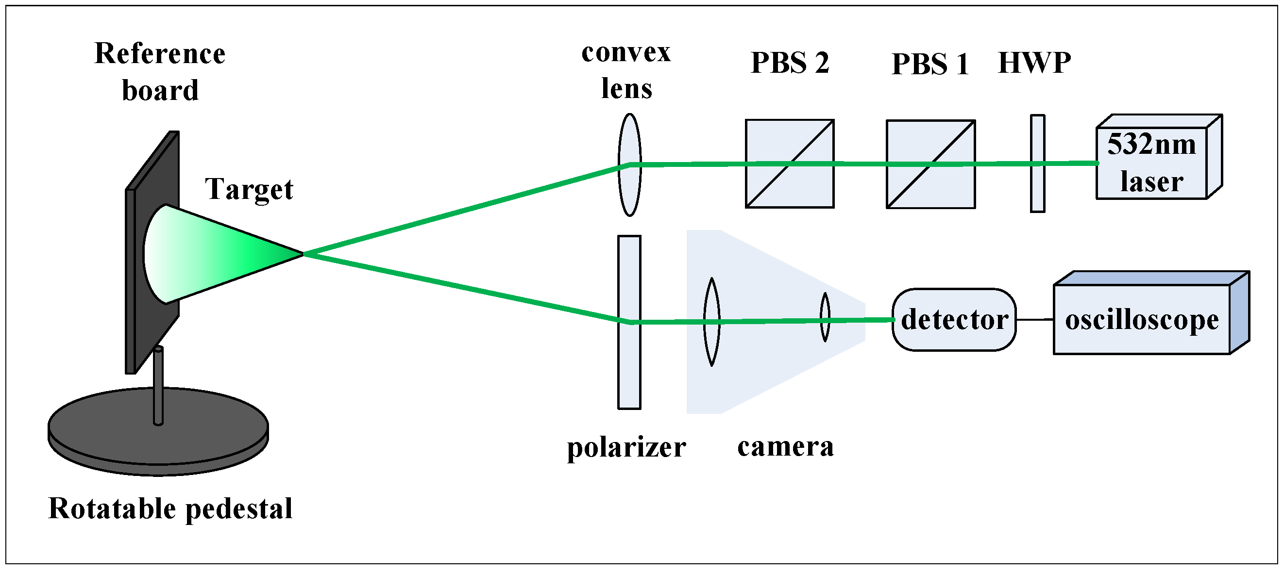
2. Method
2.1. General Theories of pBRDF
2.1.1. Specular Component
2.1.2. Diffuse Component
3. Theoretical Calculations
3.1. General Planar Surfaces
3.2. Disc
3.3. Rectangle
3.4. Typical Curved Surfaces
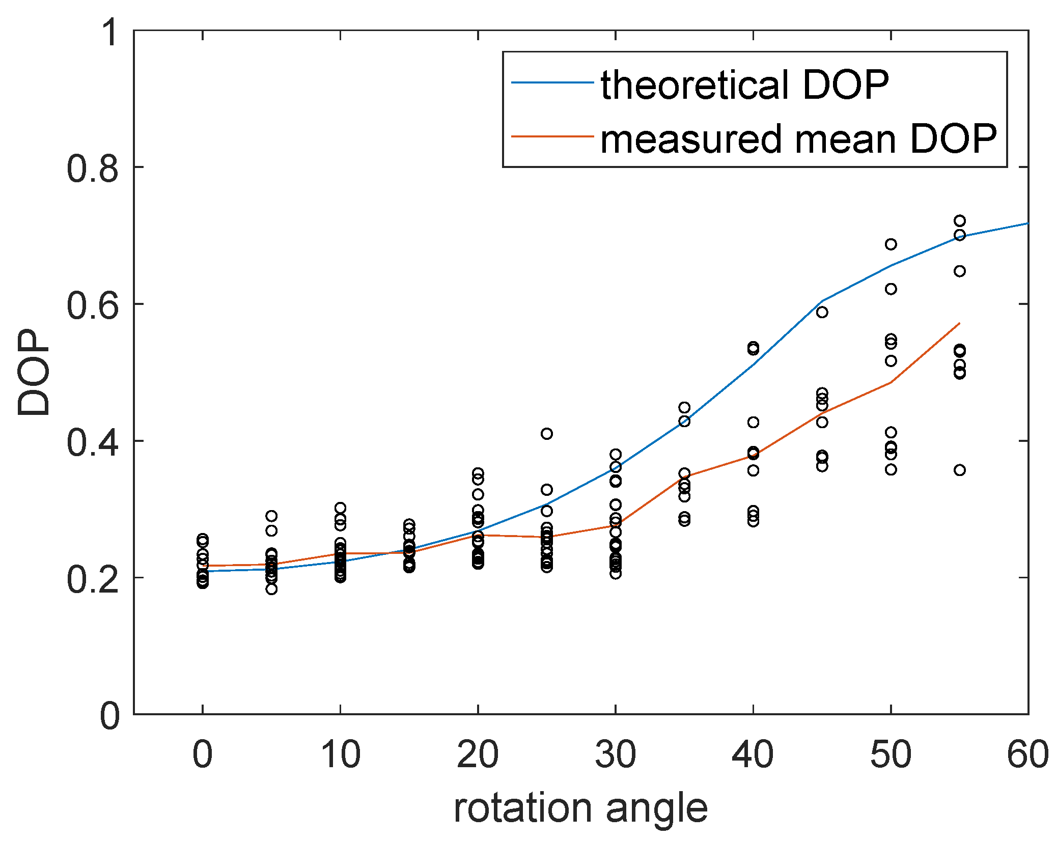
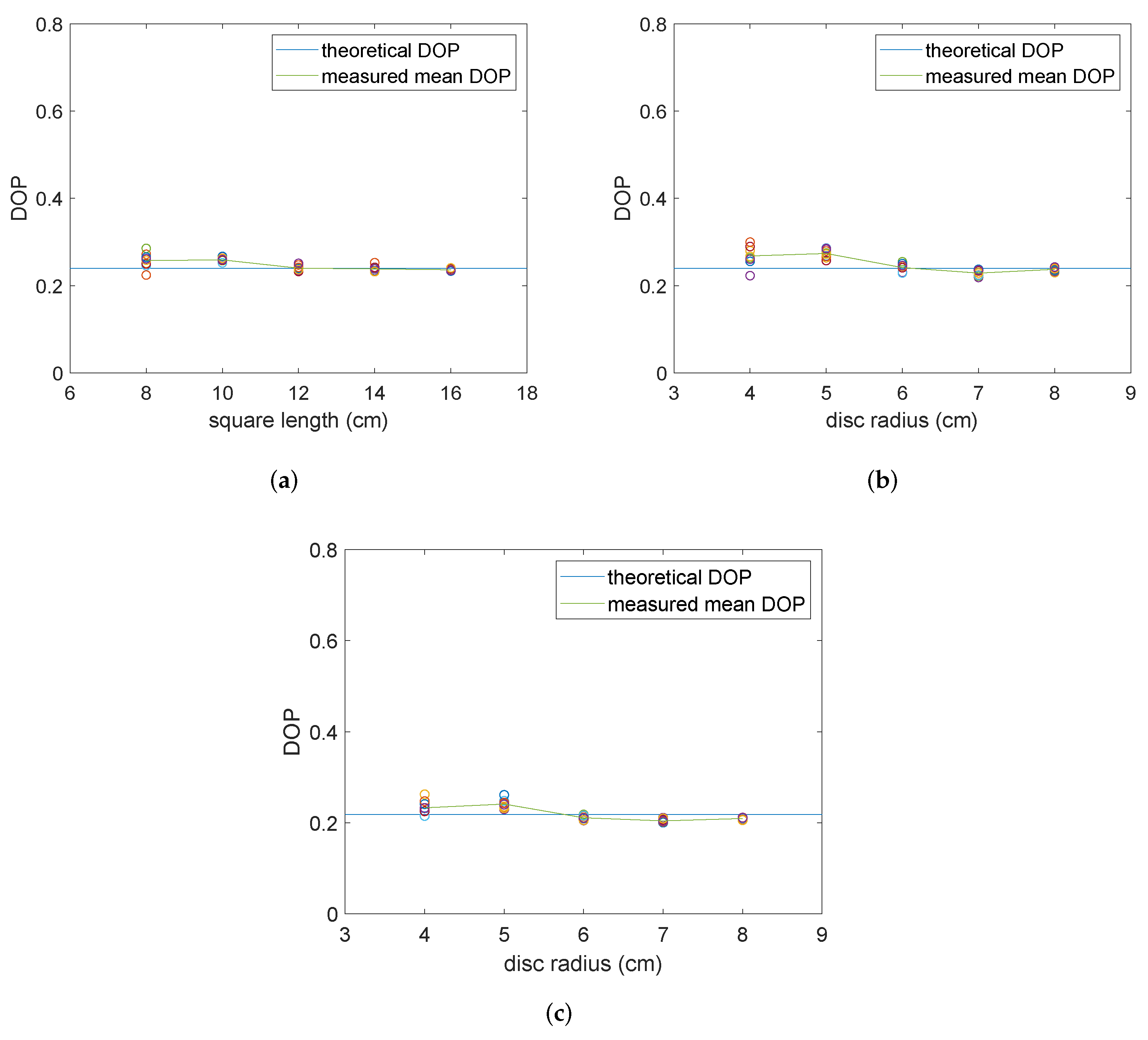
4. Results
5. Discussion
6. Conclusions
Author Contributions
Funding
Conflicts of Interest
References
- Ratliff, B.M.; LeMaster, D.A.; Mack, R.T.; Villeneuve, P.V.; Weinheimer, J.J.; Middendorf, J.R. Detection and tracking of RC model aircraft in LWIR microgrid polarimeter data. In Polarization Science and Remote Sensing V; International Society for Optics and Photonics: Bellingham, WA, USA, 2011; Volume 8160, p. 816002. [Google Scholar]
- Gavrilov, N.; Kshevetskii, S. Verifications of the nonlinear numerical model and polarization relations of atmospheric acoustic-gravity waves. Geosci. Model Dev. Discuss. 2014, 7, 7805–7822. [Google Scholar]
- Lavigne, D.A.; Breton, M.; Fournier, G.; Charette, J.F.; Pichette, M.; Rivet, V.; Bernier, A.P. Target discrimination of man-made objects using passive polarimetric signatures acquired in the visible and infrared spectral bands. In Polarization Science and Remote Sensing V; International Society for Optics and Photonics: Bellingham, WA, USA, 2011; Volume 8160, p. 816007. [Google Scholar]
- Forssell, G.; Hedborg-Karlsson, E. Measurements of polarization properties of camouflaged objects and of the denial of surfaces covered with cenospheres. In Targets and Backgrounds IX: Characterization and Representation; International Society for Optics and Photonics: Bellingham, WA, USA, 2003; Volume 5075, pp. 246–258. [Google Scholar]
- Li, X.; Zhang, L.; Qi, P.; Zhu, Z.; Xu, J.; Liu, T.; Zhai, J.; Hu, H. Are Indices of Polarimetric Purity Excellent Metrics for Object Identification in Scattering Media? Remote Sens. 2022, 14, 4148. [Google Scholar] [CrossRef]
- Duggin, M.J.; Kinn, G.J. Vegetative target enhancement in natural scenes using multiband polarization methods. In Polarization Analysis and Measurement IV; SPIE: Bellingham, WA, USA, 2002; Volume 4481, pp. 281–291. [Google Scholar]
- Li, S.; Han, X.; Weng, F. Monitoring Land Vegetation from Geostationary Satellite Advanced Himawari Imager (AHI). Remote Sens. 2022, 14, 3817. [Google Scholar] [CrossRef]
- Zhang, Z.; Yan, L.; Jiang, X.; Ding, J.; Zhang, F.; Jiang, K.; Shang, K. Exploring the Potential of Optical Polarization Remote Sensing for Oil Spill Detection: A Case Study of Deepwater Horizon. Remote Sens. 2022, 14, 2398. [Google Scholar] [CrossRef]
- Qu, Y.; Liang, S.; Liu, Q.; He, T.; Liu, S.; Li, X. Mapping surface broadband albedo from satellite observations: A review of literatures on algorithms and products. Remote Sens. 2015, 7, 990–1020. [Google Scholar] [CrossRef] [Green Version]
- Ding, A.; Jiao, Z.; Dong, Y.; Zhang, X.; Peltoniemi, J.I.; Mei, L.; Guo, J.; Yin, S.; Cui, L.; Chang, Y.; et al. Evaluation of the snow albedo retrieved from the snow kernel improved the Ross-Roujean BRDF model. Remote Sens. 2019, 11, 1611. [Google Scholar] [CrossRef] [Green Version]
- Shaw, J.A. Degree of linear polarization in spectral radiances from water-viewing infrared radiometers. Appl. Opt. 1999, 38, 3157–3165. [Google Scholar] [CrossRef]
- Hieronymi, M. Polarized reflectance and transmittance distribution functions of the ocean surface. Opt. Express 2016, 24, A1045–A1068. [Google Scholar] [CrossRef]
- Touzi, R.; Hurley, J.; Vachon, P.W. Optimization of the degree of polarization for enhanced ship detection using polarimetric RADARSAT-2. IEEE Trans. Geosci. Remote Sens. 2015, 53, 5403–5424. [Google Scholar] [CrossRef]
- Zhang, Y.; Xuan, J.; Zhao, H.; Song, P.; Zhang, Y.; Xu, W. Improved atmospheric effect elimination method for the roughness estimation of painted surfaces. Opt. Lett. 2018, 43, 1079–1082. [Google Scholar] [CrossRef]
- Li, J.; Qiu, S.; Zhang, Y.; Yang, B.; Gao, C.; Qian, Y.; Liu, Y.; Zhao, Y. Assessment of BRDF Impact on VIIRS DNB from Observed Top-of-Atmosphere Reflectance over Dome C in Nighttime. Remote Sens. 2021, 13, 301. [Google Scholar] [CrossRef]
- Guo, R.; Jiang, Z.; Jin, Z.; Zhang, Z.; Zhang, X.; Guo, L.; Hu, Y. Reflective Tomography Lidar Image Reconstruction for Long Distance Non-Cooperative Target. Remote Sens. 2022, 14, 3310. [Google Scholar] [CrossRef]
- Brown, A.J.; Michaels, T.I.; Byrne, S.; Sun, W.; Titus, T.N.; Colaprete, A.; Wolff, M.J.; Videen, G.; Grund, C.J. The case for a modern multiwavelength, polarization-sensitive LIDAR in orbit around Mars. J. Quant. Spectrosc. Radiat. Transf. 2015, 153, 131–143. [Google Scholar] [CrossRef] [Green Version]
- Brown, A.J. Equivalence relations and symmetries for laboratory, LIDAR, and planetary Müeller matrix scattering geometries. JOSA A 2014, 31, 2789–2794. [Google Scholar] [CrossRef] [PubMed]
- Dong, Q.; Huang, Z.; Li, W.; Li, Z.; Song, X.; Liu, W.; Wang, T.; Bi, J.; Shi, J. Polarization Lidar Measurements of Dust Optical Properties at the Junction of the Taklimakan Desert–Tibetan Plateau. Remote Sens. 2022, 14, 558. [Google Scholar] [CrossRef]
- Kong, Z.; Yin, Z.; Cheng, Y.; Li, Y.; Zhang, Z.; Mei, L. Modeling and evaluation of the systematic errors for the polarization-sensitive imaging lidar technique. Remote Sens. 2020, 12, 3309. [Google Scholar] [CrossRef]
- Brown, A.J. Spectral curve fitting for automatic hyperspectral data analysis. IEEE Trans. Geosci. Remote Sens. 2006, 44, 1601–1608. [Google Scholar] [CrossRef] [Green Version]
- Wen, N.; Zeng, F.; Dai, K.; Li, T.; Zhang, X.; Pirasteh, S.; Liu, C.; Xu, Q. Evaluating and Analyzing the Potential of the Gaofen-3 SAR Satellite for Landslide Monitoring. Remote Sens. 2022, 14, 4425. [Google Scholar] [CrossRef]
- Yang, M.; Xu, W.; Sun, Z.; Jia, A.; Xiu, P.; Chen, W.; Li, L.; Zheng, C.; Li, J. Degree of polarization modeling based on modified microfacet pBRDF model for material surface. Opt. Commun. 2019, 453, 124390. [Google Scholar] [CrossRef]
- Shen, Y.; Chen, B.; He, C.; He, H.; Guo, J.; Wu, J.; Elson, D.S.; Ma, H. Polarization Aberrations in High-Numerical-Aperture Lens Systems and Their Effects on Vectorial-Information Sensing. Remote Sens. 2022, 14, 1932. [Google Scholar] [CrossRef]
- Liang, J.; Ren, L.; Ju, H.; Zhang, W.; Qu, E. Polarimetric dehazing method for dense haze removal based on distribution analysis of angle of polarization. Opt. Express 2015, 23, 26146–26157. [Google Scholar] [CrossRef] [PubMed]
- Wang, X.; Hu, T.; Li, D.; Guo, K.; Gao, J.; Guo, Z. Performances of polarization-retrieve imaging in stratified dispersion media. Remote Sens. 2020, 12, 2895. [Google Scholar] [CrossRef]
- Nicodemus, F.E. Directional reflectance and emissivity of an opaque surface. Appl. Opt. 1965, 4, 767–775. [Google Scholar] [CrossRef]
- Torrance, K.E.; Sparrow, E.M. Theory for off-specular reflection from roughened surfaces. Josa 1967, 57, 1105–1114. [Google Scholar] [CrossRef]
- Nicodemus, F.E.; Richmond, J.C.; Hsia, J.J.; Ginsberg, I.; Limperis, T. Geometrical considerations and nomenclature for reflectance. NBS Monogr. 1992, 160, 4. [Google Scholar]
- Leader, J. Bidirectional scattering of electromagnetic waves from rough surfaces. J. Appl. Phys. 1971, 42, 4808–4816. [Google Scholar] [CrossRef]
- Beckmann, P.; Spizzichino, A. The Scattering of Electromagnetic Waves from Rough Surfaces; Artech House, Inc.: Norwood, MA, USA, 1987. [Google Scholar]
- Valenzuela, G. Depolarization of EM waves by slightly rough surfaces. IEEE Trans. Antennas Propag. 1967, 15, 552–557. [Google Scholar] [CrossRef]
- Barrick, D. Rough surface scattering based on the specular point theory. IEEE Trans. Antennas Propag. 1968, 16, 449–454. [Google Scholar] [CrossRef]
- Flynn, D.S.; Alexander, C. Polarized surface scattering expressed in terms of a bidirectional reflectance distribution function matrix. Opt. Eng. 1995, 34, 1646–1650. [Google Scholar]
- Priest, R.G.; Meier, S.R. Polarimetric microfacet scattering theory with applications to absorptive and reflective surfaces. Opt. Eng. 2002, 41, 988–993. [Google Scholar] [CrossRef]
- Hyde, M.W., IV; Schmidt, J.D.; Havrilla, M.J. A geometrical optics polarimetric bidirectional reflectance distribution function for dielectric and metallic surfaces. Opt. Express 2009, 17, 22138–22153. [Google Scholar] [CrossRef] [PubMed]
- Zhan, H.; Voelz, D.G. Modified polarimetric bidirectional reflectance distribution function with diffuse scattering: Surface parameter estimation. Opt. Eng. 2016, 55, 123103. [Google Scholar] [CrossRef]
- Renhorn, I.G.; Hallberg, T.; Bergström, D.; Boreman, G.D. Four-parameter model for polarization-resolved rough-surface BRDF. Opt. Express 2011, 19, 1027–1036. [Google Scholar] [CrossRef] [PubMed]
- Renhorn, I.G.; Hallberg, T.; Boreman, G.D. Efficient polarimetric BRDF model. Opt. Express 2015, 23, 31253–31273. [Google Scholar] [CrossRef] [PubMed]
- Liu, H.; Zhu, J.; Wang, K.; Xu, R. Polarized BRDF for coatings based on three-component assumption. Opt. Commun. 2017, 384, 118–124. [Google Scholar] [CrossRef]
- Rowe, M.; Pugh, E.; Tyo, J.S.; Engheta, N. Polarization-difference imaging: A biologically inspired technique for observation through scattering media. Opt. Lett. 1995, 20, 608–610. [Google Scholar] [CrossRef]
- Lavigne, D.A.; Breton, M.; Pichette, M.; Larochelle, V.; Simard, J.R. Evaluation of active and passive polarimetric electro-optic imagery for civilian and military targets discrimination. In Polarization: Measurement, Analysis, and Remote Sensing VIII; SPIE: Bellingham, WA, USA, 2008; Volume 6972, pp. 285–293. [Google Scholar]
- Vermeulen, A.; Devaux, C.; Herman, M. Retrieval of the scattering and microphysical properties of aerosols from ground-based optical measurements including polarization. I. Method. Appl. Opt. 2000, 39, 6207–6220. [Google Scholar] [CrossRef]
- Sun, Y. Statistical ray method for deriving reflection models of rough surfaces. JOSA A 2007, 24, 724–744. [Google Scholar] [CrossRef]
- Liu, H.; Zhu, J.; Wang, K. Modified polarized geometrical attenuation model for bidirectional reflection distribution function based on random surface microfacet theory. Opt. Express 2015, 23, 22788–22799. [Google Scholar] [CrossRef]
- Sun, L.; Zhao, F. Geometric attenuation factor based on scattering theory from randomly rough surface. Appl. Opt. 2021, 60, 476–483. [Google Scholar] [CrossRef]
- Shen, S.; Zhang, X.; Liu, Y.; Fang, J.; Xu, S.; Hu, Y. Calculation of Stokes vector of laser backscattering from typical geometric rough surfaces at a long distance. Appl. Opt. 2022, 61, 1766–1777. [Google Scholar] [CrossRef] [PubMed]
- Kalantari, E.; Molan, Y.E. Analytical BRDF model for rough surfaces. Optik 2016, 127, 1049–1055. [Google Scholar] [CrossRef]
- Zhang, Y.; Zhang, Y.; Zhao, H.; Wang, Z. Improved atmospheric effects elimination method for pBRDF models of painted surfaces. Opt. Express 2017, 25, 16458–16475. [Google Scholar] [CrossRef] [PubMed]
- Jiang, Y.; Li, Z. Mueller matrix of laser scattering by a two-dimensional randomly rough surface. J. Quant. Spectrosc. Radiat. Transf. 2022, 287, 108225. [Google Scholar] [CrossRef]
- Prokopenko, V.; Alekseev, S.; Matveev, N.; Popov, I. Simulation of the polarimetric bidirectional reflectance distribution function. Opt. Spectrosc. 2013, 114, 961–964. [Google Scholar] [CrossRef]
- Wang, S.; Xue, L.; Yan, K. Numerical calculation of light scattering from metal and dielectric randomly rough Gaussian surfaces using microfacet slope probability density function based method. J. Quant. Spectrosc. Radiat. Transf. 2017, 196, 183–200. [Google Scholar] [CrossRef]
- Letnes, P.A.; Maradudin, A.A.; Nordam, T.; Simonsen, I. Calculation of the Mueller matrix for scattering of light from two-dimensional rough surfaces. Phys. Rev. A 2012, 86, 031803. [Google Scholar] [CrossRef]


| Squares | Discs | Cones | ||
|---|---|---|---|---|
| Length | Radius | Radius | Height | |
| 8 cm | 4 cm | 4 cm | 2 cm | 63 |
| 10 cm | 5 cm | 5 cm | 2.5 cm | 63 |
| 12 cm | 6 cm | 6 cm | 3 cm | 63 |
| 14 cm | 7 cm | 7 cm | 3.5 cm | 63 |
| 16 cm | 8 cm | 8 cm | 4 cm | 63 |
Publisher’s Note: MDPI stays neutral with regard to jurisdictional claims in published maps and institutional affiliations. |
© 2022 by the authors. Licensee MDPI, Basel, Switzerland. This article is an open access article distributed under the terms and conditions of the Creative Commons Attribution (CC BY) license (https://creativecommons.org/licenses/by/4.0/).
Share and Cite
Shen, S.; Zhang, X.; Liu, Y.; Xu, S.; Fang, J.; Hu, Y. Degree of Polarization Calculation for Laser Backscattering from Typical Geometric Rough Surfaces at Long Distance. Remote Sens. 2022, 14, 6001. https://doi.org/10.3390/rs14236001
Shen S, Zhang X, Liu Y, Xu S, Fang J, Hu Y. Degree of Polarization Calculation for Laser Backscattering from Typical Geometric Rough Surfaces at Long Distance. Remote Sensing. 2022; 14(23):6001. https://doi.org/10.3390/rs14236001
Chicago/Turabian StyleShen, Shiyang, Xinyuan Zhang, Yifan Liu, Shilong Xu, Jiajie Fang, and Yihua Hu. 2022. "Degree of Polarization Calculation for Laser Backscattering from Typical Geometric Rough Surfaces at Long Distance" Remote Sensing 14, no. 23: 6001. https://doi.org/10.3390/rs14236001