Article

Assessing the Accuracy of Landsat Vegetation Fractional Cover for Monitoring Australian Drylands

1
Earth and Sustainability Science Research Centre, School of Biological, Earth and Environmental Sciences, University of New South Wales, Sydney, NSW 2052, Australia
2
School of Science, Western Sydney University, Locked Bag 1797, Penrith, NSW 2751, Australia
*
Author to whom correspondence should be addressed.
Remote Sens. 2022, 14(24), 6322; https://doi.org/10.3390/rs14246322
Submission received: 24 October 2022 / Revised: 12 December 2022 / Accepted: 12 December 2022 / Published: 13 December 2022
(This article belongs to the Special Issue Remote Sensing for Surface Biophysical Parameter Retrieval)

Abstract

:
Satellite-derived vegetation fractional cover (VFC) has shown to be a promising tool for dryland ecosystem monitoring. This model, calibrated through biophysical field measurements, depicts the sub-pixel proportion of photosynthetic vegetation (PV), non-photosynthetic vegetation (NPV) and bare soil (BS). The distinction between NPV and BS makes it particularly important for drylands, as these fractions often dominate. Two Landsat VFC products are available for the Australian continent: the original Joint Remote Sensing Research Program (JRSRP) product, and a newer Digital Earth Australia (DEA) product. Although similar validation statistics have been presented for each, an evaluation of their differences has not been undertaken. Moreover, spatial variability of VFC accuracy within drylands has not been comprehensively assessed. Here, a large field dataset (4207 sites) was employed to compare Landsat VFC accuracy across the Australian continent, with detailed spatial and temporal analysis conducted on four regions of interest. Furthermore, spatiotemporal features of VFC unmixing error (UE) were explored to characterize model uncertainty in large areas yet to be field sampled. Our results showed that the JRSRP and DEA VFC were very similar (RMSE = 4.00–6.59) and can be employed interchangeably. Drylands did not show a substantial difference in accuracy compared to the continental assessment; however contrasting variations were observed in dryland subtypes (e.g., semi-arid and arid zones). Moreover, VFC effectively tracked total ground cover change over time. UE increased with tree cover and height, indicating that model uncertainty was low in typical dryland landscapes. Together, these results provide guiding points to understanding the Australian ecosystems where VFC can be used with confidence.

1. Introduction

Multi-spectral remote sensing of vegetation has proved to be an exceptionally useful tool for long-term ecological monitoring at multiple scales and relatively low cost [1,2,3,4]. Several vegetation monitoring applications rely on spectral indices (e.g., normalized, enhanced and soil adjusted vegetation indices, among others) that exploit the particularities of photosynthetic vegetation (PV) reflectance (i.e., high absorption in the visible red, high reflection in the near infra-red) [4,5,6]. In dryland environments, these indices tend not to be suitable for characterizing the ecosystem condition, as senescent/non-photosynthetic vegetation (NPV) often dominates the landscape [7,8,9]. Normalized difference vegetation index (NDVI) values, for instance, have been shown to be similar for NPV and bare soil (BS) [10]. As NDVI and other indices are not robust descriptors of vegetation structure in these environments, alternative models should be considered, such as those calibrated with field biophysical measurements.
Vegetation fractional cover (VFC) can be defined as the sub-pixel proportion of PV, NPV and BS [11,12,13]. VFC has been modelled from multi-spectral satellite data through several approaches (Table 1 in [14,15,16,17]) and has been employed in many studies involving vegetation dynamics [18,19,20,21,22,23,24,25,26,27,28,29,30,31,32,33]. Scarth et al. [13] developed the first spectral unmixing model to be routinely applied to imagery at continental [14,34] and global [35,36] scales. This model relies on extensive field data to derive endmembers and unmix Landsat/MODIS imagery to obtain VFC at a spatial resolution of 30 m and 500 m, respectively [13,14]. This study focuses on the continental scale Landsat VFC products, which have several advantages compared to the MODIS products: the calibration–validation data better matches Landsat data spatially [37]; the long archive of Landsat data in Australia extends back to 1987; and the image resolution allows applications at a finer scale, such as looking at within-paddock variations.
The accuracy of Landsat VFC models for the Australian continent has been assessed through comparison against field data [14,34]. Two models with slight methodological differences have been published and validated (Table 1): one by the Joint Remote Sensing Research Program (JRSRP) [14], and another by Digital Earth Australia (DEA) [34]. The former has been applied to nation-wide [38,39] and state-wide vegetation monitoring programs [40,41], and has been utilized in local and regional scale studies [13,18,19,24,30], whereas DEA VFC has been employed in continental land cover mapping [32], and mangrove dynamics monitoring [29]. Both products report similar overall root mean square error (RMSE) (Table 1). JRSRP and DEA VFC are similar, as they both use algorithms after Scarth et al. [13], though they differ in the methods for pre-processing the satellite imagery (Table 1) resulting in unequal validation results. These differences also mean that the two products disagree up to 5% for BS and NPV, and less than 10% for PV [34], although further analysis of these differences has not been conducted.
Distinguishing the differences in spectral signals from NPV and BS can be particularly difficult in drylands [10,13,25,42,43,44]. Endmembers for NPV and BS appear to be highly correlated, especially in arid zones (i.e., correlation coefficient of 0.82 for the Australian arid zone [25]). The difficulty in separating BS and NPV has been attributed to high soil brightness in arid and semi-arid areas [42], which also have large bare soil fractions that can override the spectral signals from sparse vegetation [43]. However, Guerschman et al. [14] found weak negative relations between model error and soil brightness in bare soil dominated areas (i.e., BS > 50%). Inaccurate estimation of NPV substantially hinders the applications of VFC, especially for those that rely on total ground cover (i.e., monitoring erosion risk [26]) and even more so in ecosystems dominated by non-green vegetation [18,19,24].
Table 1. Published validation results for Joint Remote Sensing Research Program’s (JRSRP) and Digital Earth Australia’s (DEA) vegetation fractional cover algorithms. (BRDF: bidirectional reflectance distribution function, RMSE: root mean square error, PV: photosynthetic vegetation, NPV: non-photosynthetic vegetation, BS: bare soil).
ProducerTechnical
Differences
Overall RSMERMSE
PV
RMSE
NPV
RMSE
BS
Reference
JRSRPBRDF, atmospheric and topographic
correction of Landsat imagery following Flood et al. [45]
11.6%11.2%16.2%13.0%[14]
DEABRDF, atmospheric and topographic
correction of Landsat imagery following Li, et al. [46,47]
11.9%11.9%17.1%14.2%[34]
Specific validation analyses of VFC in some areas of Australian drylands have been published, generally reporting decreased estimation accuracy [24,25,48]. Melville et al. [48] found JRSRP’s algorithm to be more accurate at detecting PV compared to NPV and BS when considering a subset of 20 field sites in Fowler’s Gap Arid Zone Research Station. More recently, a recalibration of JRSRP’s algorithm for the Australian arid zone (Figure 1a) using 1405 field calibration/validation sites [25], increased accuracy for all three fractions compared to the original products. Nonetheless, a comprehensive assessment of VFC in drylands across the Australian continent is required to illustrate its effectiveness and encourage more applications. The analyses presented here were designed to address this gap and answer the following questions: (1) How different are the JRSRP and DEA VFC image products? (2) How does the accuracy of the VFC unmixing model change within drylands? (3) How well do the endmembers represent the land cover in Australian drylands?

2. Materials and Methods
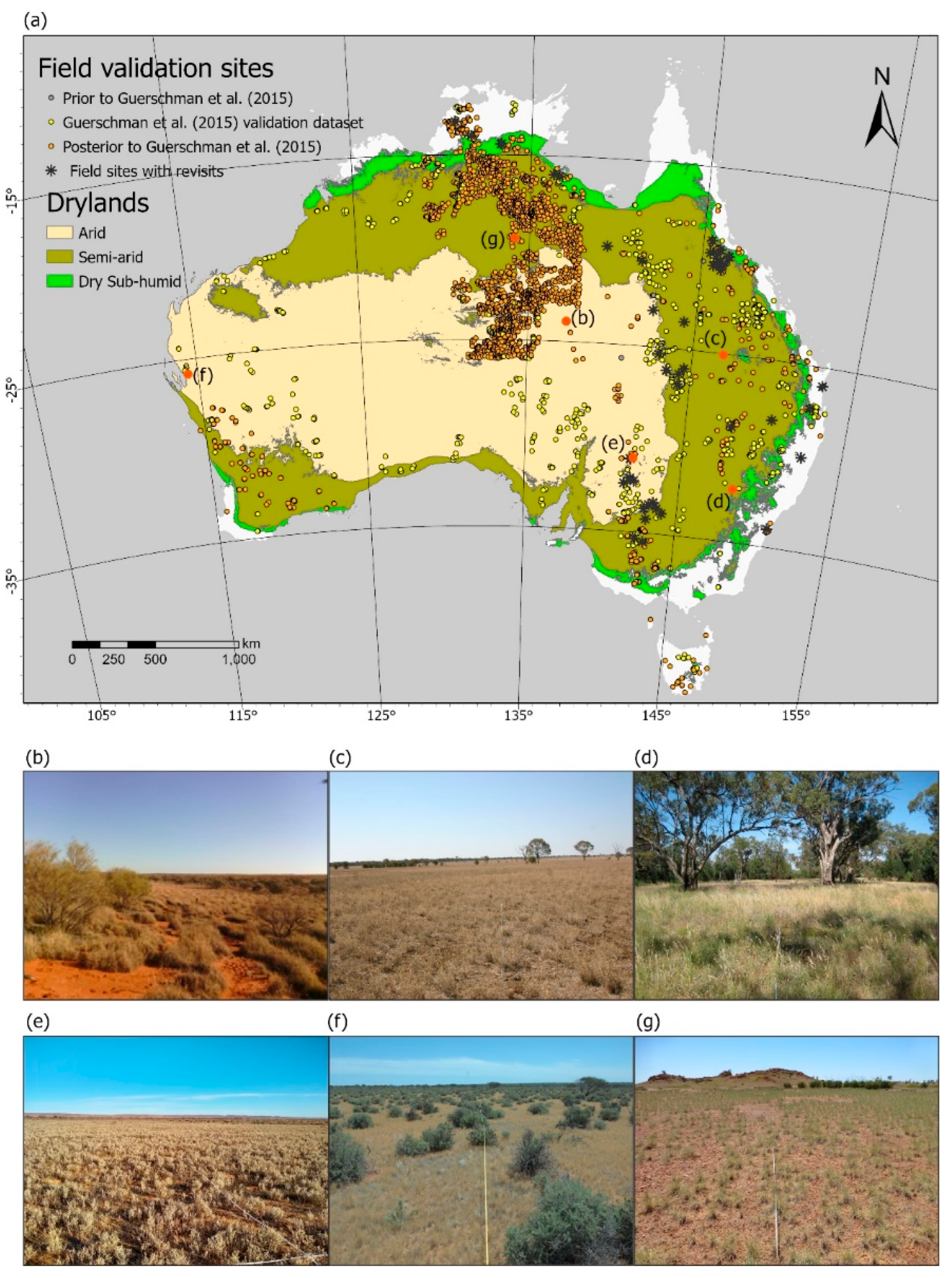
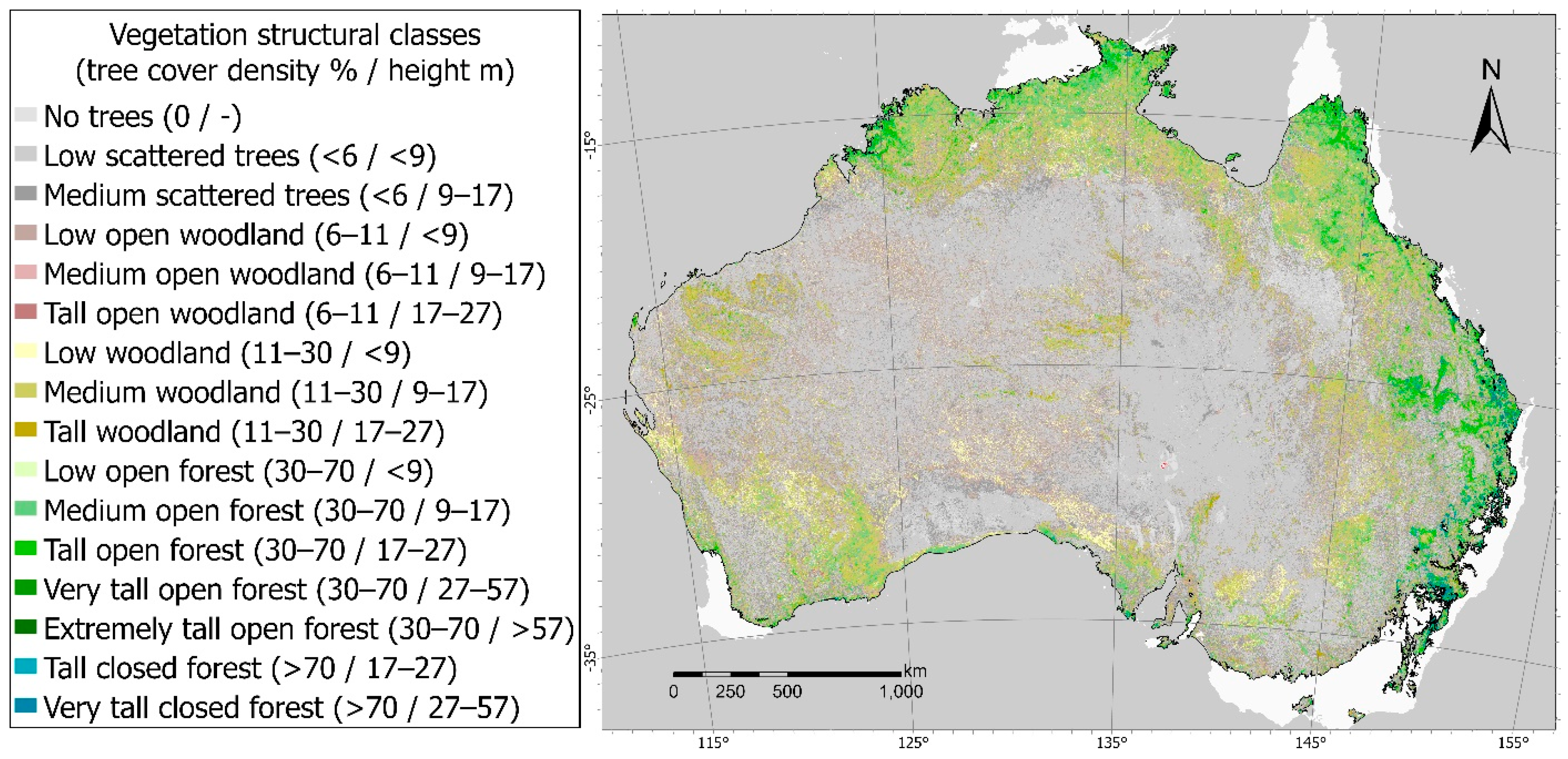
2.1. Study Area

Drylands dominate the Australian continent, covering 90% when mapped according to the average aridity index for the period 1976–2005 [49] (Figure 1a). The aridity index was calculated as the relation of precipitation to potential evapotranspiration after the following thresholds: 0.05 ≤ arid < 0.2 ≤ semi-arid < 0.5 ≤ dry sub-humid < 0.65. Vegetation cover in Australian drylands is dominated by several types of grasslands, shrublands, and open woodlands [50] (Figure 1b–g).

2.2. Datasets

A continental field dataset following the State-wide Landcover and Tree Study (SLATS) protocol [37] was obtained from the Queensland Government Department of Environment and Science [51]. This dataset contained 4207 unique observations in time (i.e., 435 site revisits are considered separate individual observations) where ground, mid and over storey cover were recorded through star-transects within ~1-hectare circular plots. The observations span from February 1997 to June 2021 and are spread throughout Australia (Figure 1a). The dataset also included the JRSRP unmixed fractional cover values from the cloud-free Landsat (5, 7 or 8) image closest to the field observation date of the 3 × 3 pixels area overlapping each plot [14].
DEA’s Landsat Collection 3 products were also employed in the analyses. These two products are ‘DEA Fractional Cover’ [34] and ‘DEA Water Observations’ [52]. Both products are derived from Landsat surface reflectance archives consisting of imagery obtained by the multispectral sensors aboard Landsat 5, 7 and 8. The water observations product was used to mask cloud, cloud shadow and water from the image archive. The reader is referred to Mueller et al. [53] for details on the production and applications of ‘DEA Water Observations’ product.
Additionally, a raster layer of vegetation structure over the Australian continent (Figure 2) [54] was used to analyse the distribution and magnitude of the unmixing error. This dataset integrated Landsat 5 and 7, Advanced Land Observing Satellite (ALOS) Phased Arrayed L-band Synthetic Aperture Radar (PALSAR) and Ice, Cloud, and land Elevation (ICESat), and Geoscience Laser Altimeter System (GLAS) data, at a spatial resolution of 30 m (matching VFC datasets derived from Landsat imagery). In contrast to other widely used vegetation structure maps of Australia (e.g., The National Vegetation Information System’s Major Vegetation Groups Map), this dataset is spatially continuous and consistent in scale and detail across the entire continent [55].

2.3. Methodological Framework

The datasets described above were processed and combined for 3 different analyses (Figure 3). Firstly, JRSRP and DEA VFC products were compared to understand their similarities and differences (Section 2.3.1). Secondly, the SLATS field dataset was employed to explore spatial and temporal properties of JRSRP VFC accuracy (Section 2.3.2). Thirdly, the DEA VFC was employed for exploring the model’s uncertainty across drylands through the unmixing error band (Section 2.3.2).

2.3.1. JRSRP and DEA VFC Comparison

The comparison of JRSRP and DEA vegetation fractional cover was based on the SLATS dataset. Raw field data (i.e., ground, mid and overstorey measurements) were processed following Guerschman et al. [14] to obtain the proportion of PV, NPV and BS. To match JRSRP VFC values in the SLATS dataset, DEA VFC was extracted following a similar method (already processed fractional cover values were directly extracted instead of extracting surface reflectance and applying the unmixing algorithm afterwards). Mean and standard deviation of the pixels overlapping the 100-m diameter plots were extracted from the cloud, cloud shadow and water-free image closest to the field observation date. Only image dates within 60 days (prior or after) the field observations and with at least 75% valid pixels were considered. Since the image filtering and extracting methods were not the same as the SLATS dataset, the number of pixels included and the dates of the images were occasionally different. On average, DEA extractions for each plot included 0.41 (σ2 = 0.91) fewer pixels than JRSRP and were obtained 0.31 (σ2 = 7.49) days later. Moreover, 61 sites were discarded from the analysis as no DEA VFC images matching the criteria above could be identified.
Accuracy assessments were undertaken for both products using the field-measured cover fractions. The statistics employed to characterize accuracy were RMSE for each fraction and the overall product (i.e., root mean of the mean square error across the 3 fractions), where errors are the difference between measured and estimated. Similarity analyses comparing extracted values of both products included scatterplots for each cover fraction; RMSE (where ‘errors’ are the difference between estimations); bias (calculated as the mean difference between DEA and JRSRP predicted cover fractions); and Pearson’s correlation coefficient (r). 95% confidence intervals were determined for RMSE and bias assuming χ2 and t-student distributions, respectively. As the RMSE interval tends to be asymmetric, the limit further from the mean was employed to simplify notation (i.e., estimated RMSE ± distance to further limit).

2.3.2. Field Validation of VFC Accuracy

Spatial variability in VFC accuracy across drylands was analysed using the SLATS star-transects field calibration–validation dataset [50], divided into 3 subsets (drylands, semi-arid zone, and arid zone) defined using the aridity index thresholds previously described (Figure 1a). The validation statistics employed for the analysis were RMSE (where errors are the difference between observed and predicted), bias (calculated as the mean difference between observed and predicted cover fractions) and Pearson’s correlation coefficient (r). 95% confidence intervals were determined for RMSE and bias in the same way as Section 2.3.1.
Temporal variability in accuracy across drylands was analysed to assess VFC’s power of detection of ground cover changes over time. The complete dataset was subset following 2 criteria: locations sampled at least twice, and showing large bare soil estimation error (i.e., a difference of at least 15% between measured and estimated BS in one or more image). The subset of sites with repeated measures consisted of 133 sites (and a total 527 observations—Figure 1a), 51 of which displayed large BS errors. Change in field-measured and satellite estimated bare soil was calculated as the difference between the value at a given date and the previous observation. Time difference between subsequent field measurements spanned from 1 day to over 16 years, with a median of 162 days (i.e., close to 5 months). For ease of interpretation, bare soil change was transformed to ground cover change following
Ground   cover   change = ( BS t BS t 1 ) × 1
where BS is the bare soil fraction; subscript t identifies an observation on a given date and t−1 the immediately previous observation. A linear regression was fitted between field-measured and VFC ground cover change and validation statistics (RMSE, bias, and r) were calculated. The 95% confidence intervals were determined for RMSE and bias in the same way as Section 2.3.1.
To assess ground cover trend detection, the proportion of observations for which measured and estimated ground cover change direction significantly disagreed was calculated. Change direction disagreements were identified as differences in sign between measurement and estimation (i.e., whether positive and negative, or positive/negative and 0). The disagreement was considered significant when the absolute difference was over 5%.

2.3.3. Unmixing Error Analysis

There is a considerable area of Australia yet to be field-sampled and which is, therefore, not represented in calibration or validation of the algorithms (Figure 1a). Some of these areas may be different enough to those that are sampled that the quality of VFC products is unknown. This section of the analysis explored an alternative method to assess the quality of VFC across the Australian drylands including unsampled and poorly sampled regions.
Both JRSRP and DEA VFC provide a quality assessment band depicting the unmixing error of the model. This error is determined by the vector of residuals between the modelled (mixture of endmembers) and observed spectra [25]. The values in the unmixing error band are calculated as the Euclidean norm of the residual vector [56]. Thus, the unmixing error can be interpreted as a measure of how well the endmembers characterize the spectral response of each pixel of an unmixed image. The unmixing error does not replace validation analyses, nevertheless, it provides some information on the model’s uncertainty.
To analyse the quality of DEA’s Landsat fractional cover in the Australian drylands, the spatial distribution of the unmixing error band values were explored in contrasting periods of time. Two annual median composites were created for the Australian drylands. The years 2016 and 2019 were selected for the analysis due to the contrasting rainfall records across the continent: 2016 showed records of above average rainfall (Figure A1) while the contrary was true for 2019 (Figure A2). A quality filter from DEA Water Observations product [52] was applied to the image collection, discarding pixels affected by cloud cover, shadow, and water following Mueller et al. [53]. A total of 30,170 DEA datasets were collected for 2016 and 30,766 for the year 2019. A composite image was prepared for each of these years using the median unmixing error value of each image pixel in the dataset. Spatial statistics (mean, standard deviation, maximum and minimum) of the unmixing error were computed, and the composites were reclassified to highlight areas where unmixing error was at least one standard deviation greater than the mean. Error patterns were explored visually to assess anecdotal observations of larger unmixing errors in densely forested areas and an analysis of correlation between unmixing error values and vegetation structural classes [55] was performed. The reference vegetation structure dataset (Section 2.2) represents the year 2009, so it was assumed that no widespread changes in structural classes across Australian drylands occurred between 2009 and 2019.
The SLATS field dataset (Section 2.2) was used to fit linear regressions between unmixing error and field-measured fractions to explore factors underlying spatial patterns. Lastly, correlation between unmixing error and estimation errors (RMSEs of each fraction and overall) were tested to examine possible relationships between model uncertainty and prediction accuracy.

3. Results

3.1. JRSRP and DEA Landsat Fractional Cover

Field validation results were similar for the JRSRP and DEA products (Table 2), suggesting that differences in image pre-processing do not have a considerable effect on the final unmixed imagery. DEA VFC showed a slightly lower accuracy (i.e., higher RMSE values) overall and for two out of three cover fractions, and a marginally higher accuracy at detecting green vegetation compared to JRSRP VFC. The importance of these differences is negligible when comparing their magnitude to the confidence intervals (Table 2).
Direct comparisons of JRSRP and DEA estimations showed they were extremely similar for all cover fractions (Figure 3). Modelled cover fractions appear to be highly correlated (r ≥ 0.94), while the difference in estimations were consistently low (RMSE ≤ 6.66) and unbiased (−1.01 ≤ bias ≤ 1.92). The highest correlation and lowest difference between predictions were found for PV, while the opposite is true for NPV. Nonetheless, estimations of the dead fraction showed the lowest bias (−0.87), as DEA predictions tend to be higher than JRSRP for lower NPV values and conversely for high NPV values (evidenced by the slope and origin of linear fit in relation to the 1:1 agreement in Figure 4). Bias for BS (PV) shows values further from 0, as DEA estimations are consistently higher (lower) than those of the JRSRP product.

3.2. Field Validation Statistics

3.2.1. Spatial Variability

Validation statistics obtained for the SLATS dataset were consistent across spatial categories (Figure 5). The green vegetation fraction had the lowest error (7.02 ≤ RMSE ≤ 10.61) and highest correlation (0.78 < r < 0.88) when considering the continental dataset, drylands, and subregions within drylands. In all cases, PV was followed by BS and NPV in increasing (decreasing) RMSE (correlation) order. Bias, conversely, was consistently closer to 0 for the bare soil fraction (−0.53 ≤ bias ≤ 0.70), suggesting that the model does not systematically overestimate or underestimate total vegetation cover. Slight overestimation and underestimation of PV and NPV, respectively, was identified for most categories.
When analysing each fraction separately, some variability was detected across the field dataset and subsets. Results for the continental and dryland subsets were approximately equal; however, subtle differences in model accuracy were observed for subregions within drylands. Both PV and NPV were most accurately estimated in the arid zone (bottom centre and right charts in Figure 5). Nonetheless, the difference in PV accuracy compared to other regions and levels was larger than in NPV. The arid zone also displayed the highest RMSE for the bare soil fraction. Moreover, the correlation coefficients in this area were the lowest across all regions and levels for the three fractions. In contrast, the semi-arid zone showed the lowest accuracy and highest bias for PV estimation compared to all other regions and levels.

3.2.2. Change Detection

Ground cover change was reasonably estimated for sites with small and large BS estimation errors. For sites where the bare soil fraction was consistently well estimated, observed and satellite derived ground cover change were highly correlated (r = 0.86) and similar (RMSE = 6.76) (Figure 6a). In contrast, locations where high error was detected at least once, displayed substantially higher RMSE (Figure 6b). Nevertheless, these sites also presented a positive and high correlation (r = 0.78) which denotes agreement between measured and estimated ground cover change. In both cases, bias was not significantly different to 0, indicating no systematic under or overestimation of change. Moreover, significant errors in trend detection were found in 15.71% and 17.16% of change observations for small error and large error sites, respectively. This is reflected in the proportion of points in Figure 6a,b falling on quadrats II and IV.

3.3. Unmixing Error Analysis

The unmixing error (UE) appears low and relatively homogeneous over space and time. The spatial mean unmixing error was 10.11% for the wet year (2016) and 9.19% for the dry year (2019). As UE depicts the distance between input and model-fitted spectra, these results show that, on average, the spectral response of the pixels across time and space was close to 90% of the spectra fitted by the unmixing model. Nonetheless, a degree of spatial heterogeneity was evident, with comparable spatial patterns of distribution in both years (Figure 7). These patterns of spatial variability also resulted in similar unmixing variance for 2016 (σ = 3.24 %) and 2019 (σ = 3.14%).
The clustered spatial distribution of relatively high UE values in distinct patches suggests that the model quality may be influenced by non-random characteristics of the surface. UE values tend to be higher near the dryland’s boundary for both years (Figure 8). The spatial distribution of these error patterns matches the distribution of landscapes with high tree cover density (i.e., forests) and over 15 m of height (Figure 2) [55]. The unmixing error consistently increased in response to shifts in tree density classes (Figure 8). Within each tree cover density class, there is a positive UE response to height class shift. This is particularly evident for the height class shift from “very tall” (mean UE = 18.31%) to “extremely tall” (mean UE = 27.91%) within the “Open Forest” tree cover density class (Figure 9). Moreover, moderate yet significant correlations (p < 0.01) were found between unmixing error and the observed cover fractions (except with NPV). The unmixing error tended to increase with the proportion of green vegetation, and more weakly decrease as the bare soil fraction increased (Figure A3).
Although the unmixing error depicts the model’s uncertainty, it was found not to be strongly linked to accuracy errors detected through field validation. A significant (p < 0.01), but low correlation (|r| < 0.18) was found between unmixing errors and absolute errors for each fraction as well as with the mean absolute error (average of absolute error for the three fractions) (Table 3). These results evidence that unmixing error does not equate to prediction error.

4. Discussion

4.1. Comparison of JRSRP and DEA VFC

Remarkably small differences were found between JRSRP and DEA vegetation fractional cover. It had been reported [34] that these products typically disagree up to 5% for BS and NPV, and less than 10% for PV. The results of this research (Figure 4) were opposite, as similarity was higher for PV and lower for NPV and BS. Furthermore, the differences presented in Table 2 and Figure 4 may not only be due to image pre-processing, but also because the methods employed for extracting DEA VFC (Section 2.3.1) are slightly different compared to those of the SLATS dataset [14].
Comparison of VFC unmixing results has been undertaken through different methods. Flood [57,58], for example, carried out pixelwise assessments to understand the effect of different sensors (i.e., Enhanced Thematic Mapper, Operational Land Imager, and Multi Spectral Instrument) on deriving surface reflectance and on the result of applying the unmixing model of Scarth et al. [13]. Both studies analysed close to 100 Landsat scenes covering Eastern Australia and timespans not greater than 18 months. Although this study used fewer pixels, they were sampled from across the whole Australian continent, and covered a timespan close to 25 years.

4.2. Variability in VFC Estimation Accuracy

The validation results obtained for the continental scale (Figure 5) were moderately different to previously published accuracy metrics (Table 1). Specifically, when comparing RMSE values, VFC was approximately 1.5% and 0.9% less accurate at detecting, respectively, non-green vegetation and bare soil, and close to 1.3% more accurate for green vegetation than that reported by Guerschman et al. [14]. Moreover, slightly decreased correlation (except PV) and increased bias were evident for the three fractions. These differences could be attributed to a significant increase in the number of observations: from approximately 1100 employed for calibration and cross-validation in Guerschman et al. (2015) to over 4200 used to calculate validation statistics in this study. Newly visited sites might contain spectral values different to the calibration data of the model and result in weaker measured performance. For instance, the observations of the newer field dataset tend to have smaller PV (median of 9.53% vs 17%) fraction, and a larger NPV (54.46% vs 45%) fraction [14]. It is assumed, however, that the updated set of observations better depict the variability in surface properties across the Australian continent, as it represents a much larger sample. Thus, the validation statistics presented in this article provide an enhanced estimation of VFC performance.
Equivalent validation results were obtained for the continental and continental drylands levels. This is closely related to the fact that over 90% of Australia’s landmass is classified as arid, semi-arid, or subhumid [59]. Accordingly, the dryland subset of field observations consists of almost 92% of the complete dataset. The most significant change, although subtle, was increased accuracy for the NPV fraction. These results disagree with findings in other dryland regions across the world [42,43], but concur with previously described [14] slightly smaller estimation errors recorded in dry and bright bare (BS > 50%) soils of Australia.
Spatial variability in VFC accuracy was evident within drylands. The arid zone displayed the smallest RMSE value for PV, while the opposite was true for the semi-arid zone (Figure 5) This difference may be attributed to the fact that both measured and estimated PV values tend to be clustered near 0 for the arid zone, while the distribution is more disperse in the semi-arid zone (Figure 5). A similar, less pronounced effect was detected for BS, which could also be related to the difference in observed BS fractions between these subsets (median of 18.75% in the semi-arid zone vs median of 46.79% in the arid zone).
Performing model validation at large scale may have ignored the effects of localized variability. For example, the differences in PV and BS detection accuracy described above became diffuse when characterizing the whole drylands region. This issue has been also reported in the literature. For instance, Melville et al. [48] detected larger inaccuracies related to NPV overestimation and BS underestimation in a small area (20 SLATS field observations) within Broken Hill Complex (arid zone). Conversely, Shumack et al. [25] observed that Landsat VFC overestimated BS and PV, and underestimated NPV when compared to classified imagery obtained through an Uncrewed Aircraft System (UAS) in 4 sites within the Simpson desert. These authors found that the VFC model could be locally enhanced by deriving endmembers from a subset of ~1400 field observations within the arid zone. However, their regional scale cross-validation results (Figure 4d in [25]) were not substantially different to those presented here (bottom row of Figure 5).

4.3. Change Detection

Accuracy in estimation of ground cover change corresponded with accuracy of individual observations. Namely, large error sites showed higher RMSE values both for individual observations and change between two subsequent timestamps. However, both subsets (large error sites and small error sites) displayed high correlations between estimations and measurements, and a low proportion of erroneous trend detection. Thus, despite the relatively large prediction error, the results confirm vegetation fractional cover modelled from Landsat satellite time series can effectively detect changes in ground cover through time (i.e., from 1 day to over 16 years in this research). These findings might not be representative of the entire Australian territory, as the field sites visited more than once are geographically limited to the central-northern and eastern portions of the country (Figure 1a). Nonetheless, these sites are well distributed across climate zones, as there are sites in arid, semi-arid, dry subhumid, and humid areas.
The results presented here support the use of Landsat VFC timeseries for monitoring ground cover in drylands at broad scale (i.e., regional/continental). Prior studies have identified inconsistencies and unexpected responses of the PV fraction to conditioning factors such as rainfall, specifically in arid environments [18,19,25]. However, landscapes in this region tend to be dominated by BS and NPV, which could explain why ground cover change was correctly estimated in most of the sites in this study. Moreover, timeseries analysis of Landsat VFC has also been successfully employed to monitor local scale effects of grazing management [13,24]. Occasional erroneous trend detection identified in this research (Figure 6), and the mentioned issues reported in the literature highlight that careful evaluation should be undertaken before employing Landsat VFC for local temporal analysis.

4.4. Unmixing Error

Two different factors likely explain the unmixing error response to vegetation structural complexity: the correlation between unmixing error and the PV fraction, and the presence of shadows. Analysis performed for this research showed that field-measured photosynthetic cover (PV) correlated positively with the unmixing error of the images (Section 3.3, Figure A3a). For instance, a 10% increase in field-measured PV is paired with a marginal 1.58% rise of unmixing error, which could explain higher unmixing error values in a wet year (2016) compared to a dry year (2019). However, this does not fully account for unmixing error variability (r2 = 0.47). One hypothesis that could explain the variance further is related to the shading effects of tree cover density and height in the landscape. Shading affects surface spectral signals by generally reducing reflectance values [60,61], consequently decreasing the ability of the selected endmembers to characterize the surface composition. A common solution to this problem has been to include an additional ‘shadow’ endmember in the spectral unmixing model [10,44,62]. However, such an approach does not resolve the issue of uncertainty related to ground cover estimation because of further limitations of linear spectral unmixing. First, due to its spectral behaviour, the shadow endmember would likely be highly correlated with other endmembers. Moreover, Landsat imagery may not have sufficient and/or relevant bands to unmix the four endmembers. It should be noted that the current three-endmember spectral unmixing model relies on additional synthetic bands to satisfactorily unmix BS, PV and NPV [13,14,25]. Furthermore, the field calibration/validation dataset does not include shadow proportion measurements and using a generic shadow endmember would significantly alter the methodological approach of this field observation-calibrated model. Lastly, even if the proportion of shade could be unmixed, information on the surface that the shadows are being cast on would be missing, thus the total proportion of BS, PV, and NPV within the pixel would still be unknown.

5. Conclusions

JRSRP and DEA VFC image products can be used interchangeably, increasing the possibility of different users accessing this valuable dryland monitoring tool. Each product has its own advantages and disadvantages. JRSRP VFC is readily available as seasonal composites (i.e., one image every 3 months), making it appropriate for time series decomposition and analyses of long-term change. DEA VFC, on the other hand, is available at a higher temporal frequency, making it more useful for monitoring short-term change.
The accuracy of vegetation fractional cover derived from Landsat images over the Australian continent was shown to be variable over space and time. Our results provide guiding points to understanding the Australian ecosystems where VFC can be used with confidence. At continental and drylands levels, accuracy is similar, suggesting that there are no further limitations on their applicability to studies of vegetation dynamics over the entire dryland ecosystem of Australia. However, it was found that the accuracy of modelled cover fractions varied within drylands. Our results suggest that although large estimation errors may occur, Landsat VFC can effectively track ground cover trends in different environments. Future versions of the continental VFC dataset based on additional validation datasets and a new machine learning approaches [63] are expected to overcome some of the limitations discussed in this paper.
VFC is a suitable tool for monitoring ground cover across large areas and conditions. This study revealed that the model’s uncertainty is generally low in drylands. Vegetation structure complexity (i.e., tree cover density and height) explained much of the spatial distribution of comparatively high unmixing errors recorded from the time series of Landsat images used. Landscapes with sparse/low tree cover show a very low model uncertainty.

Author Contributions

Conceptualization, A.S., G.M. and A.F.; methodology, A.S., G.M. and A.F.; software, A.S.; validation, A.S.; formal analysis, A.S.; investigation, A.S.; resources, A.S. and A.F.; data curation, A.S.; writing—original draft preparation, A.S.; writing—review and editing, G.M. and A.F.; visualization, A.S. All authors have read and agreed to the published version of the manuscript.

Funding

This research received no external funding.

Institutional Review Board Statement

Not applicable.

Informed Consent Statement

Not applicable.

Data Availability Statement

The following publicly available datasets were analyzed in this study. SLATS star-transects data be found here: https://field.jrsrp.com/, accessed on 15 June 2022. DEA fractional cover data can be found here: https://cmi.ga.gov.au/data-products/dea/629/dea-fractional-cover-landsat#access, accessed on 15 June 2022. Vegetation height and tree density can be found here: https://dap.tern.org.au/thredds/catalog/landscapes/remote_sensing/spatial_other/jrsrp/height/catalog.html, accessed on 20 July 2022.

Acknowledgments

The authors would like to thank the following groups for providing free and open data: United States Geological Survey, Joint Remote Sensing Research Program Geoscience Australia, and the Terrestrial Ecosystem Research Network (TERN) infrastructure, which is enabled by the Australian Government’s National Collaborative Research Infrastructure Strategy (NCRIS). This research is supported by an Australian Government Research Training Program (RTP) Scholarship.

Conflicts of Interest

The authors declare no conflict of interest.

Appendix A

Figure A1. 2016 rainfall deciles in Australian continent. Source: Bureau of Meteorology (http://www.bom.gov.au/climate/history/rainfall/, accessed on 20 September 2022).
Remotesensing 14 06322 g0a1
Figure A2. 2019 rainfall deciles in Australian continent. Source: Bureau of Meteorology (http://www.bom.gov.au/climate/history/rainfall/, accessed on 20 September 2022).
Remotesensing 14 06322 g0a2
Figure A3. Scatter plots of field-measured (a) photosynthetic vegetation and (b) bare soil fractions (%) against unmixing error (%). The dashed line represents the linear fit between the variables. Intercept and slope were significant with p < 0.0000001 in both cases (n = 4207).
Remotesensing 14 06322 g0a3

References

  1. Pettorelli, N.; Owen, H.J.F.; Duncan, C. How do we want Satellite Remote Sensing to support biodiversity conservation globally? Methods Ecol. Evol. 2016, 7, 656–665. [Google Scholar] [CrossRef]
  2. Pettorelli, N.; Wegmann, M.; Skidmore, A.; Mücher, S.; Dawson, T.P.; Fernandez, M.; Lucas, R.; Schaepman, M.E.; Wang, T.; O’Connor, B. Framing the concept of satellite remote sensing essential biodiversity variables: Challenges and future directions. Remote Sens. Ecol. Conserv. 2016, 2, 122–131. [Google Scholar] [CrossRef]
  3. Skidmore, A.K.; Pettorelli, N.; Coops, N.C.; Geller, G.N.; Hansen, M.; Lucas, R.; Mücher, C.A.; O’Connor, B.; Paganini, M.; Pereira, H.M. Environmental science: Agree on biodiversity metrics to track from space. Nat. News. 2015, 523, 403. [Google Scholar] [CrossRef] [PubMed] [Green Version]
  4. Xue, J.; Su, B. Significant remote sensing vegetation indices: A review of developments and applications. J. Sens. 2017, 1-17, 1–17. [Google Scholar] [CrossRef] [Green Version]
  5. Gao, F.; Hilker, T.; Zhu, X.; Anderson, M.; Masek, J.; Wang, P.; Yang, Y. Fusing Landsat and MODIS Data for Vegetation Monitoring. IEEE Geosci. Remote Sens. Mag. 2015, 3, 47–60. [Google Scholar] [CrossRef]
  6. Zhang, X.; Friedl, M.A.; Schaaf, C.B.; Strahler, A.H.; Hodges, J.C.F.; Gao, F.; Reed, B.C.; Huete, A. Monitoring vegetation phenology using MODIS. Remote Sens. Environ. 2003, 84, 471–475. [Google Scholar] [CrossRef]
  7. Huete, A.R.; Jackson, R.D. Suitability of spectral indices for evaluating vegetation characteristics on arid rangelands. Remote Sens. Environ. 1987, 23, 213–218. [Google Scholar] [CrossRef]
  8. van Leeuwen, W.J.D.; Huete, A.R. Effects of standing litter on the biophysical interpretation of plant canopies with spectral indices. Remote Sens. Environ. 1996, 55, 123–138. [Google Scholar] [CrossRef]
  9. Smith, W.K.; Dannenberg, M.P.; Yan, D.; Herrmann, S.; Barnes, M.L.; Barron-Gafford, G.A.; Biederman, J.A.; Ferrenberg, S.; Fox, A.M.; Hudson, A.; et al. Remote sensing of dryland ecosystem structure and function: Progress, challenges, and opportunities. Remote Sens. Environ. 2019, 233, 111401. [Google Scholar] [CrossRef]
  10. Smith, M.O.; Ustin, S.L.; Adams, J.B.; Gillespie, A.R. Vegetation in deserts: I. A regional measure of abundance from multispectral images. Remote Sens. Environ. 1990, 31, 1–26. [Google Scholar] [CrossRef]
  11. Dennison, P.; Roberts, D.A.; Chambers, J.Q.; Daughtry, C.S.; Guerschman, J.P.; Kokaly, R.F.; Okin, C.G.S.; Scarth, P.F. Global Measurement of Non-Photosynthetic Vegetation; NASA: Washington, DC, USA, 2016.
  12. Guerschman, J.P.; Hill, M.J.; Renzullo, L.J.; Barrett, D.J.; Marks, A.S.; Botha, E.J. Estimating fractional cover of photosynthetic vegetation, non-photosynthetic vegetation and bare soil in the Australian tropical savanna region upscaling the EO-1 Hyperion and MODIS sensors. Remote Sens. Environ. 2009, 113, 928–945. [Google Scholar] [CrossRef]
  13. Scarth, P.; Röder, A.; Schmidt, M. Tracking Grazing Pressure and Climate Interaction-The Role of Landsat Fractional Cover in Time Series Analysis. In Proceedings of the 15th Australasian Remote Sensing and Photogrammetry, Alice Springs, NT, Australia, 13–17 September 2010. [Google Scholar]
  14. Guerschman, J.P.; Scarth, P.F.; McVicar, T.R.; Renzullo, L.J.; Malthus, T.J.; Stewart, J.B.; Rickards, J.E.; Trevithick, R. Assessing the effects of site heterogeneity and soil properties when unmixing photosynthetic vegetation, non-photosynthetic vegetation and bare soil fractions from Landsat and MODIS data. Remote Sens. Environ. 2015, 161, 12–26. [Google Scholar] [CrossRef]
  15. Meyer, T.; Okin, G.S. Evaluation of spectral unmixing techniques using MODIS in a structurally complex savanna environment for retrieval of green vegetation, nonphotosynthetic vegetation, and soil fractional cover. Remote Sens. Environ. 2015, 161, 122–130. [Google Scholar] [CrossRef]
  16. Tian, J.; Su, S.; Tian, Q.; Zhan, W.; Xi, Y.; Wang, N. A novel spectral index for estimating fractional cover of non-photosynthetic vegetation using near-infrared bands of Sentinel satellite. Int. J. Appl. Earth Obs. Geoinf. 2021, 101, 102361. [Google Scholar] [CrossRef]
  17. Wang, G.; Wang, J.; Zou, X.; Chai, G.; Wu, M.; Wang, Z. Estimating the fractional cover of photosynthetic vegetation, non-photosynthetic vegetation and bare soil from MODIS data: Assessing the applicability of the NDVI-DFI model in the typical Xilingol grasslands. Int. J. Appl. Earth Obs. Geoinf. 2019, 76, 154–166. [Google Scholar] [CrossRef]
  18. Fisher, A.; Hesse, P.P. The response of vegetation cover and dune activity to rainfall, drought and fire observed by multitemporal satellite imagery. Earth Surf. Process. Landf. 2019, 44, 2957–2967. [Google Scholar] [CrossRef]
  19. Fisher, A.; Mills, C.H.; Lyons, M.; Cornwell, W.K.; Letnic, M. Remote sensing of trophic cascades: Multi-temporal landsat imagery reveals vegetation change driven by the removal of an apex predator. Landsc. Ecol. 2021, 36, 1341–1358. [Google Scholar] [CrossRef]
  20. Gray, J.M.; Karunaratne, S.; Bishop, T.; Wilson, B.; Veeragathipillai, M. Driving factors of soil organic carbon fractions over New South Wales, Australia. Geoderma. 2019, 353, 213–226. [Google Scholar] [CrossRef]
  21. Jackson, H.; Prince, S.D. Degradation of Non-Photosynthetic Vegetation in a Semi-Arid Rangeland. Remote Sens. 2016, 8, 692. [Google Scholar] [CrossRef] [Green Version]
  22. Scarth, P.; Trevithick, R. Management effects on ground cover “clumpiness”: Scaling from field to Sentinel-2 cover estimates. Int. Arch. Photogramm. Remote Sens. Spat. Inf. Sci. 2017, 183–188. [Google Scholar] [CrossRef]
  23. Wang, B.; Waters, C.; Orgill, S.; Gray, J.; Cowie, A.; Clark, A.; Liu, D.L. High resolution mapping of soil organic carbon stocks using remote sensing variables in the semi-arid rangelands of eastern Australia. Sci. Total Environ. 2018, 630, 367–378. [Google Scholar] [CrossRef]
  24. Barnetson, J.; Phinn, S.; Scarth, P.; Denham, R. Assesing Landsat Fractional ground-cover time series across Aaustralia’a arid rangelands: Separating grazing impact from climate variability. Int. Arch. Photogramm. Remote Sens. Spat. Inf. Sci. 2017, 15–26. [Google Scholar] [CrossRef] [Green Version]
  25. Shumack, S.; Fisher, A.; Hesse, P.P. Refining medium resolution fractional cover for arid Australia to detect vegetation dynamics and wind erosion susceptibility on longitudinal dunes. Remote Sens. Environ. 2021, 265, 112647. [Google Scholar] [CrossRef]
  26. Guerschman, J.P.; Hill, M.J.; Leys, J.; Heidenreich, S. Vegetation cover dependence on accumulated antecedent precipitation in Australia: Relationships with photosynthetic and non-photosynthetic vegetation fractions. Remote Sens. Environ. 2020, 240, 111670. [Google Scholar] [CrossRef]
  27. Guerschman, J.P.; Leys, J.; Rozas Larraondo, P.; Henrikson, M.; Paget, M.; Barson, M. Monitoring Groundcover: An Online Tool for Australian Regions Technical Report; Australian Government Department of Agriculture and Water Resources: Canberra, ACT, Australia, 2018.
  28. Pringle, M.J.; O’Reagain, P.J.; Stone, G.S.; Carter, J.O.; Orton, T.G.; Bushell, J.J. Using remote sensing to forecast forage quality for cattle in the dry savannas of northeast Australia. Ecol. Indic. 2021, 133, 108426. [Google Scholar] [CrossRef]
  29. Lymburner, L.; Bunting, P.; Lucas, R.; Scarth, P.; Alam, I.; Phillips, C.; Ticehurst, C.; Held, A. Mapping the multi-decadal mangrove dynamics of the Australian coastline. Remote Sens. Environ. 2020, 238, 111185. [Google Scholar] [CrossRef]
  30. Thornton, C.M.; Elledge, A.E. Heavy grazing of buffel grass pasture in the Brigalow Belt bioregion of Queensland, Australia, more than tripled runoff and exports of total suspended solids compared to conservative grazing. Mar. Pollut. Bull. 2021, 171, 112704. [Google Scholar] [CrossRef]
  31. Donohue, R.J.; Mokany, K.; McVicar, T.R.; O’Grady, A.P. Identifying management-driven dynamics in vegetation cover: Applying the Compere framework to Cooper Creek, Australia. Ecosphere 2022, 13, e4006. [Google Scholar] [CrossRef]
  32. Lucas, R.; Mueller, N.; Siggins, A.; Owers, C.; Clewley, D.; Bunting, P.; Kooymans, C.; Tissott, B.; Lewis, B.; Lymburner, L.; et al. Land Cover Mapping using Digital Earth Australia. Data 2019, 4, 143. [Google Scholar] [CrossRef] [Green Version]
  33. Harwood, T.D.; Donohue, R.J.; Williams, K.J.; Ferrier, S.; McVicar, T.R.; Newell, G.; White, M. Habitat Condition Assessment System: A new way to assess the condition of natural habitats for terrestrial biodiversity across whole regions using remote sensing data. Methods Ecol. Evol. 2016, 7, 1050–1059. [Google Scholar] [CrossRef]
  34. Geoscience Australia. DEA Fractional Cover (Landsat). 2021. Available online: https://cmi.ga.gov.au/data-products/dea/629/dea-fractional-cover-landsat#details (accessed on 25 August 2021).
  35. Hill, M.J.; Guerschman, J.P. The MODIS Global Vegetation Fractional Cover Product 2001–2018: Characteristics of Vegetation Fractional Cover in Grasslands and Savanna Woodlands. Remote Sens. 2020, 12, 406. [Google Scholar] [CrossRef] [Green Version]
  36. Hill, M.J.; Guerschman, J.P. Global trends in vegetation fractional cover: Hotspots for change in bare soil and non-photosynthetic vegetation. Agric. Ecosyst. Environ. 2022, 324, 107719. [Google Scholar] [CrossRef]
  37. Muir, J.; Schmidt, M.; Tindall, D.; Trevithick, R.; Scarth, P.; Stewart, J. Field Measurement of Fractional Ground Cover: A Technical Handbook Supporting Ground Cover Monitoring for Australia; ABARES: Canberra, ACT, Australia, 2011.
  38. Leys, J.F.; Howorth, J.E.; Guerschman, J.P.; Bala, B.; Stewart, J.B. Setting Targets for National Landcare Program Monitoring and Reporting Vegetation Cover for Australia; Environment, Energy and Science: Parramatta, NSW, Australia, 2020.
  39. Beutel, T.S.; Trevithick, R.; Scarth, P.; Tindall, D. VegMachine. net. online land cover analysis for the Australian rangelands. Rangel. J. 2019, 41, 355–362. [Google Scholar] [CrossRef] [Green Version]
  40. State of New South Wales and Department of Planning and Environment. Native Vegetation Regulatory Map Method Statement; Environment, Energy and Science: Parramatta, NSW, Australia, 2022.
  41. Queensland Government Department of Environment and Science. Statewide Landcover and Trees Study–Methodology Overview; Queensland Government: Brisbane, QLD, Australia, 2021.
  42. Asner, G.P.; Heidebrecht, K.B. Spectral unmixing of vegetation, soil and dry carbon cover in arid regions: Comparing multispectral and hyperspectral observations. Int. J. Remote Sens. 2002, 23, 3939–3958. [Google Scholar] [CrossRef]
  43. Okin, G.S.; Roberts, D.A.; Murray, B.; Okin, W.J. Practical limits on hyperspectral vegetation discrimination in arid and semiarid environments. Remote Sens. Environ. 2001, 77, 212–225. [Google Scholar] [CrossRef]
  44. Roberts, D.A.; Smith, M.O.; Adams, J.B. Green vegetation, nonphotosynthetic vegetation, and soils in AVIRIS data. Remote Sens. Environ. 1993, 44, 255–269. [Google Scholar] [CrossRef]
  45. Flood, N.; Danaher, T.; Gill, T.; Gillingham, S. An Operational Scheme for Deriving Standardised Surface Reflectance from Landsat TM/ETM+ and SPOT HRG Imagery for Eastern Australia. Remote Sens. 2013, 5, 83–109. [Google Scholar] [CrossRef] [Green Version]
  46. Li, F.; Jupp, D.L.B.; Reddy, S.; Lymburner, L.; Mueller, N.; Tan, P.; Islam, A. An Evaluation of the Use of Atmospheric and BRDF Correction to Standardize Landsat Data. IEEE J. Sel. Top. Appl. Earth Obs. Remote Sens. 2010, 3, 257–270. [Google Scholar] [CrossRef]
  47. Li, F.; Jupp, D.L.B.; Thankappan, M.; Lymburner, L.; Mueller, N.; Lewis, A.; Held, A. A physics-based atmospheric and BRDF correction for Landsat data over mountainous terrain. Remote Sens. Environ. 2012, 124, 756–770. [Google Scholar] [CrossRef]
  48. Melville, B.; Fisher, A.; Lucieer, A. Ultra-high spatial resolution fractional vegetation cover from unmanned aerial multispectral imagery. Int. J. Appl. Earth Obs. Geoinf. 2019, 78, 14–24. [Google Scholar] [CrossRef]
  49. Harwood, T.; Donohue, R.; Harman, I.; McVicar, T.; Ota, N.; Perry, J.; Williams, K. 9s Climatology for Continental Australia 1976–2005: Summary Variables with Elevation and Radiative Adjustment. 2019.Version v3. Available online: https://researchdata.edu.au/9s-climatology-continental-radiative-adjustment (accessed on 30 September 2021).
  50. Australian Government Department of Agriculture, Water and the Environment. National Vegetation Information System V6.0. 2021. Available online: http://www.environment.gov.au/fed/catalog/search/resource/details.page?uuid=ab942d6d-9efd-4cf2-bec7-4c1521b83803 (accessed on 30 September 2021).
  51. Queensland Government Department of Environment and Science. SLATS Star Transects-Australian field sites. 2022.Version 1.0.0. Available online: http://geonetwork.tern.org.au/geonetwork/srv/eng/catalog.search#/metadata/24a40c29-0d7c-4fe8-bdde-9c4ea495bfb8 (accessed on 15 June 2022).
  52. Geoscience Australia. DEA Water Observations; Geoscience Australia: Symonston, ACT, Australia, 2022. [CrossRef]
  53. Mueller, N.; Lewis, A.; Roberts, D.; Ring, S.; Melrose, R.; Sixsmith, J.; Lymburner, L.; McIntyre, A.; Tan, P.; Curnow, S.; et al. Water observations from space: Mapping surface water from 25years of Landsat imagery across Australia. Remote Sens. Environ. 2016, 174, 341–352. [Google Scholar] [CrossRef] [Green Version]
  54. Joint Remote Sensing Research Program. Vegetation Height and Structure-Derived from ALOS-1 PALSAR, Landsat and ICESat/GLAS, Australia. 2022. Available online: https://portal.tern.org.au/vegetation-height-structure-australia-coverage/21777 (accessed on 20 July 2022).
  55. Scarth, P.; Armston, J.; Lucas, R.; Bunting, P. A Structural Classification of Australian Vegetation Using ICESat/GLAS, ALOS PALSAR, and Landsat Sensor Data. Remote Sens. 2019, 11, 147. [Google Scholar] [CrossRef] [Green Version]
  56. Lawson, C.L.; Hanson, R.J. Solving Least Squares Problems; SIAM: Philadelphia, PA, USA, 1995. [Google Scholar]
  57. Flood, N. Continuity of reflectance data between Landsat-7 ETM+ and Landsat-8 OLI, for both top-of-atmosphere and surface reflectance: A study in the Australian landscape. Remote Sens. 2014, 6, 7952–7970. [Google Scholar] [CrossRef] [Green Version]
  58. Flood, N. Comparing Sentinel-2A and Landsat 7 and 8 using surface reflectance over Australia. Remote Sens. 2017, 9, 659. [Google Scholar] [CrossRef] [Green Version]
  59. Prăvălie, R. Drylands extent and environmental issues. A global approach. Earth-Sci. Rev. 2016, 161, 259–278. [Google Scholar] [CrossRef]
  60. O’Neill, A.L. Satellite-derived vegetation indices applied to semi-arid shrublands in Australia. Aust. Geogr. 1996, 27, 185–199. [Google Scholar] [CrossRef]
  61. Pech, R.P.; Graetz, R.D.; Davis, A.W. Reflectance modelling and the derivation of vegetation indices for an Australian semi-arid shrubland. Int. J. Remote Sens. 1986, 7, 389–403. [Google Scholar] [CrossRef]
  62. Small, C. The Landsat ETM+ spectral mixing space. Remote Sens. Environ. 2004, 93, 1–17. [Google Scholar] [CrossRef]
  63. Joint Remote Sensing Research Program. Seasonal Fractional Cover-Landsat JRSRP Algorithm Version 3.0, Australia Coverage. 2022. Available online: https://geonetwork.tern.org.au/geonetwork/srv/eng/catalog.search;jsessionid=node010373b43998rp68arlv2t2h0r44039.node0#/metadata/0997cb3c-e2e2-45be-ac82-f5e13d24331c (accessed on 23 October 2022).
Figure 1. Vegetation in Australian drylands. (a) The location of field sample plots and drylands subdivisions across Australia. The dataset consists of 4243 field sites sampled following Muir et al. (2011); 162 were sampled previous to the dataset employed in Guerschman (1171 sites), and a further 2874 were sampled afterwards. Drylands were mapped according to the average aridity index for the period 1976–2005 (Harwood et al., 2019) after the following thresholds: 0.05 ≤ arid < 0.2 ≤ semi-arid < 0.5 ≤ dry sub-humid < 0.65. (bg) Field photographs of select field sites (b) Hummock grassland on dune slope; (c) Tussock grassland on plain; (d) Grassy woodland near creek; (e) Chenopod shrubland on plain; (f) Open scrub on plain; (g) Hummock grassland on plain. Photographs (ad) and (f,g) were obtained from https://data.tern.org.au/rs/public/data/field_validation/sitedata/, accessed on 15 September 2022, (e) was captured by the authors in May 2021.
Remotesensing 14 06322 g001
Figure 2. Vegetation structure classified according to tree density and height. Modified from Scarth et al. [55].
Remotesensing 14 06322 g002
Figure 3. Flow chart depicting the processing steps and combinations of datasets. Each section addresses a separate research question.
Remotesensing 14 06322 g003
Figure 4. Scatterplots showing JSRSP (x-axis) and DEA (y-axis) estimated fractions (%) of bare soil (left), photosynthetic vegetation (middle) and non-photosynthetic vegetation (right) for 4166 field sites. The black line represents the 1:1 agreement, the dashed line is the linear fit between both estimations.
Remotesensing 14 06322 g004
Figure 5. Scatterplots showing the field-observed (y-axis) and JRSRP-modelled (x-axis) fractions (%) of bare soil (left), photosynthetic vegetation (middle) and non-photosynthetic vegetation (right) for the Australian continent (n = 4207), drylands within Australia (n = 3876) and two of its subtypes: the semi-arid zone (n = 2116) and the arid zone (n = 1425). The black line corresponds to the 1:1 agreement, the dashed line is the linear fit between the observed and predicted values. Pearson’s correlation coefficient (r), root mean square error (RMSE), and bias (calculated as the mean difference between observed and predicted) are displayed. Confidence intervals of 95% are shown for RMSE and bias.
Remotesensing 14 06322 g005
Figure 6. Scatterplots of field-measured and modelled total ground cover (100 –bare soil fraction (%)) change across the continent. The black line corresponds to the 1:1 agreement. Dashed lines on y = 0 and x = 0 are displayed to highlight the proportion of points falling on quadrants I (+, +) and III (-, -). (a) Scatterplots of sites where BS error < 15%, n = 261 (199 in drylands). (b) Scatterplots of sites where BS error > 15% at least once, n = 134 (104 in drylands).
Remotesensing 14 06322 g006
Figure 7. Unmixing error images within drylands of (a) a wet year (2016) and (b) a dry year (2019).
Remotesensing 14 06322 g007
Figure 8. Images of distance to the mean unmixing error measured in standard deviations for (a) a wet year (2016) and (b) a dry year (2019).
Remotesensing 14 06322 g008
Figure 9. Box plots showing year 2016 (top) and year 2019 (bottom) median unmixing error distribution for 16 vegetation structural classes in Australian drylands. n > 50,000 for every structural class (Structural classes definitions in Figure 8).
Remotesensing 14 06322 g009
Table 2. Validation results (using SLATS star-transect field dataset) for Joint Remote Sensing Research Program’s (JRSRP) and Digital Earth Australia’s (DEA) vegetation fractional cover algorithms. RMSE: root mean square error (%), PV: photosynthetic vegetation, NPV: non-photosynthetic vegetation, BS: bare soil. 95% confidence intervals are shown between parentheses.

Producer
Overall
RMSE
RMSE
BS
RMSE
PV
RMSE
NPV
JRSRP14.13 (±0.31)13.83 (±0.30)9.86 (±0.21)17.61 (±0.39)
DEA14.39 (±0.32)14.28 (±0.31)9.80 (±0.21)17.93 (±0.39)
Table 3. Correlation between unmixing error and absolute model prediction error of all field sites (n = 4207).
Pearson’s Correlation Coefficientp Value
PV0.165>0.000001
NPV0.132>0.000001
BS−0.175>0.000001
Overall0.044>0.01
Publisher’s Note: MDPI stays neutral with regard to jurisdictional claims in published maps and institutional affiliations.

