

Automatic Mapping of Burned Areas Using Landsat 8 Time-Series Images in Google Earth Engine: A Case Study from Iran


Abstract
:1. Introduction
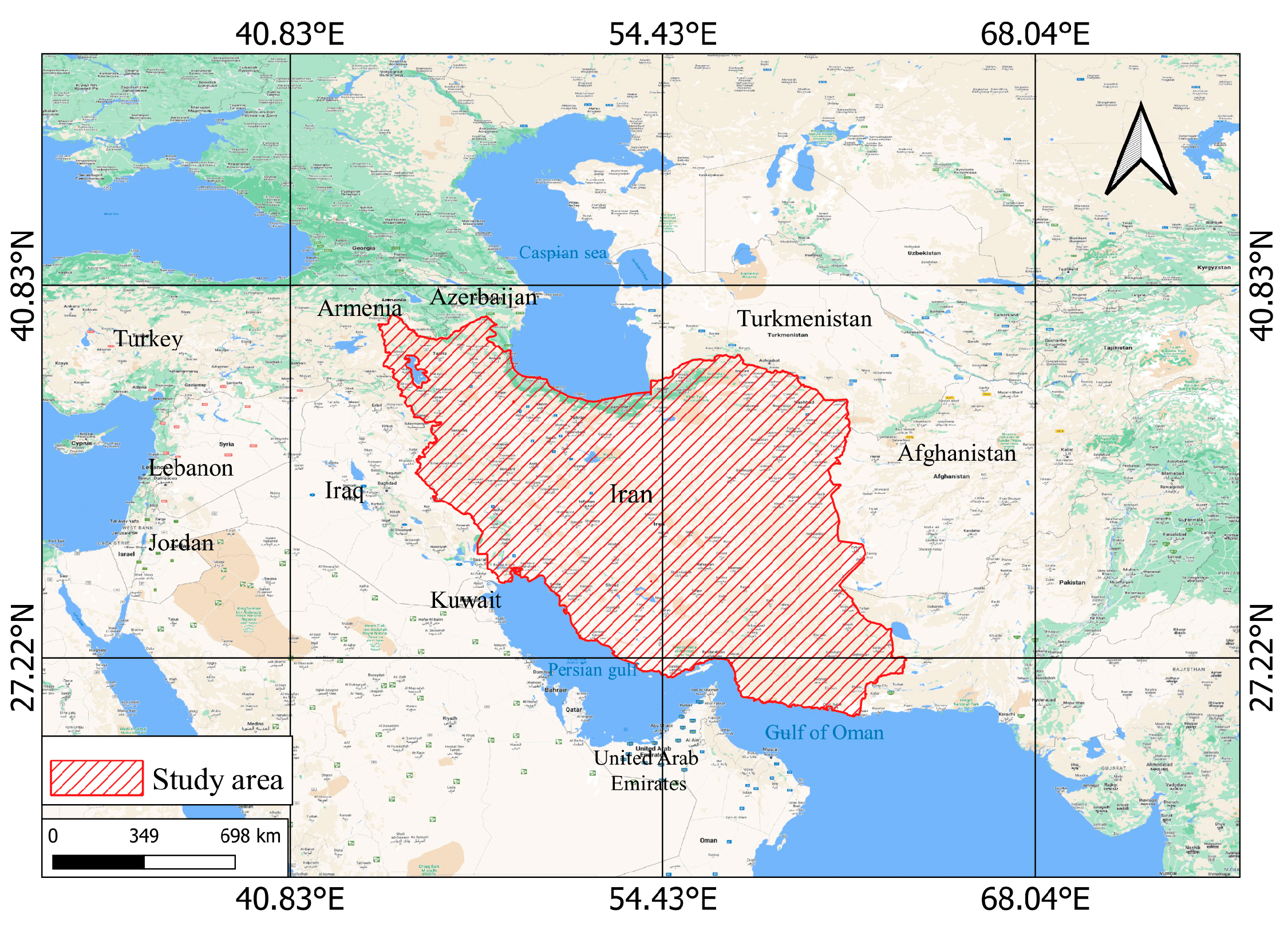
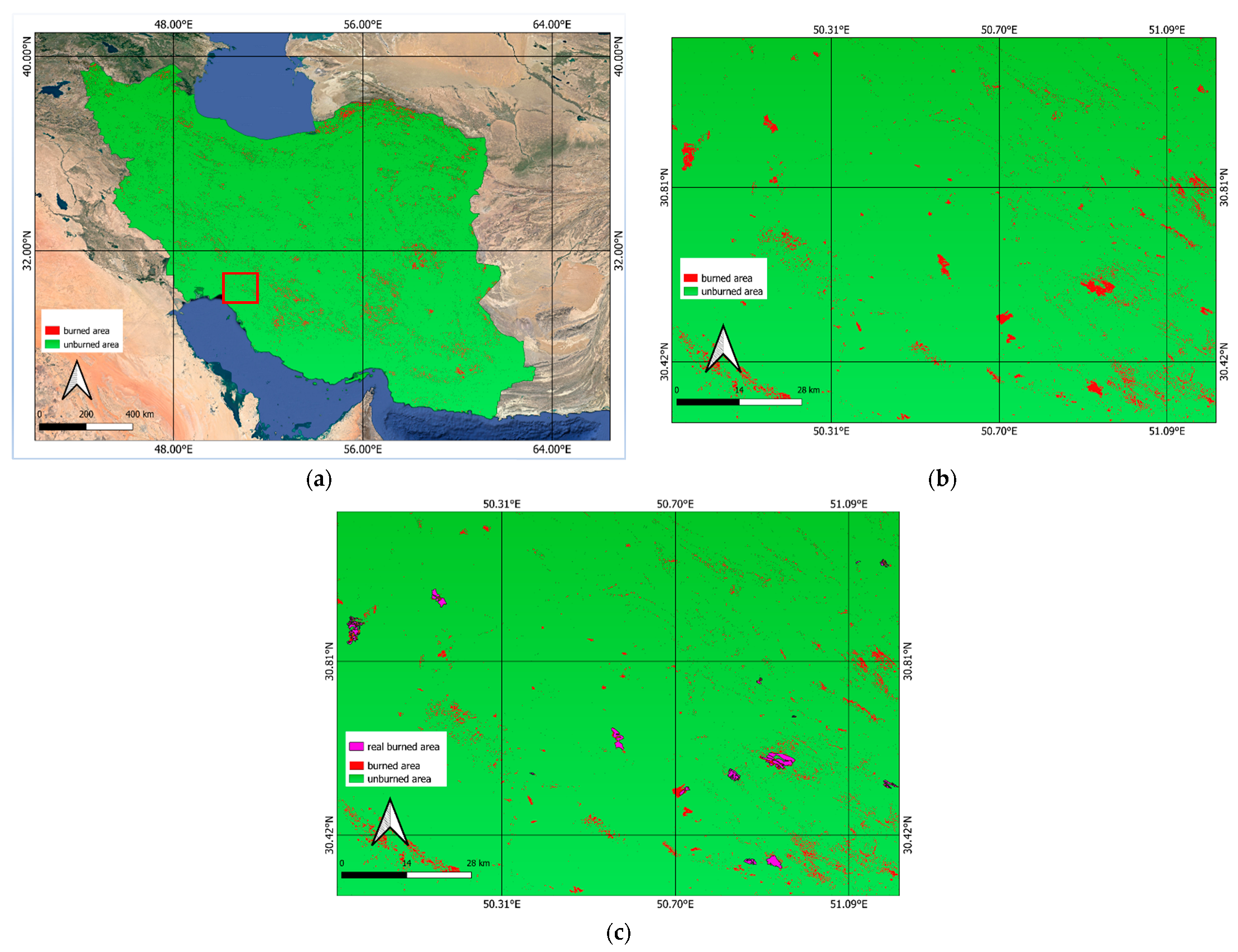
2. Study Area
3. Data
4. Materials and Methods
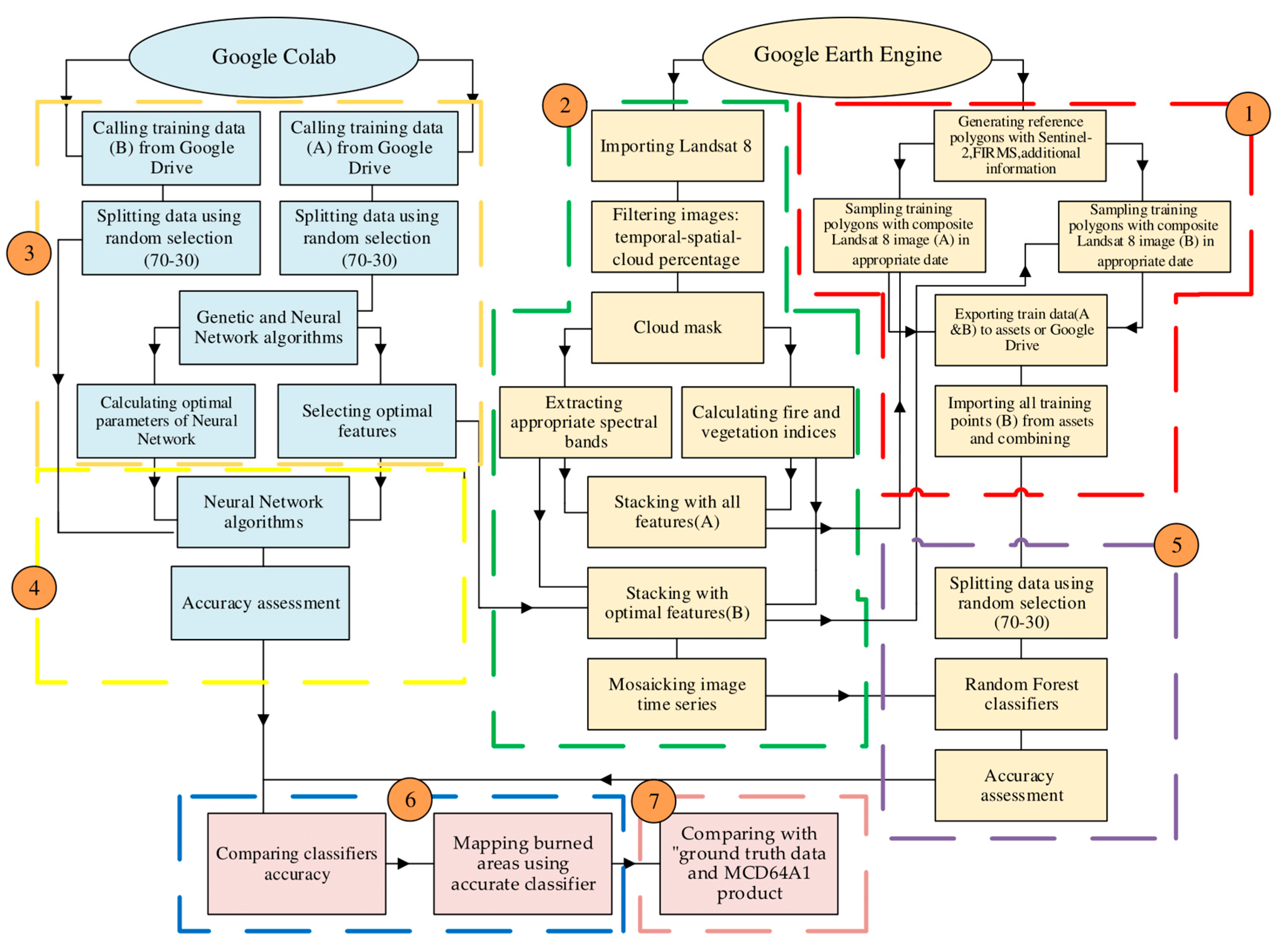
4.1. Overview
4.2. Google Earth Engine (GEE) Platform
4.3. Generating Reference Polygons
4.3.1. Burned Reference Data
4.3.2. Unburned Reference Data
4.3.3. Preparing Training Polygons
4.4. Mapping Burned Areas
4.5. Feature Selection in Google Colab Platform
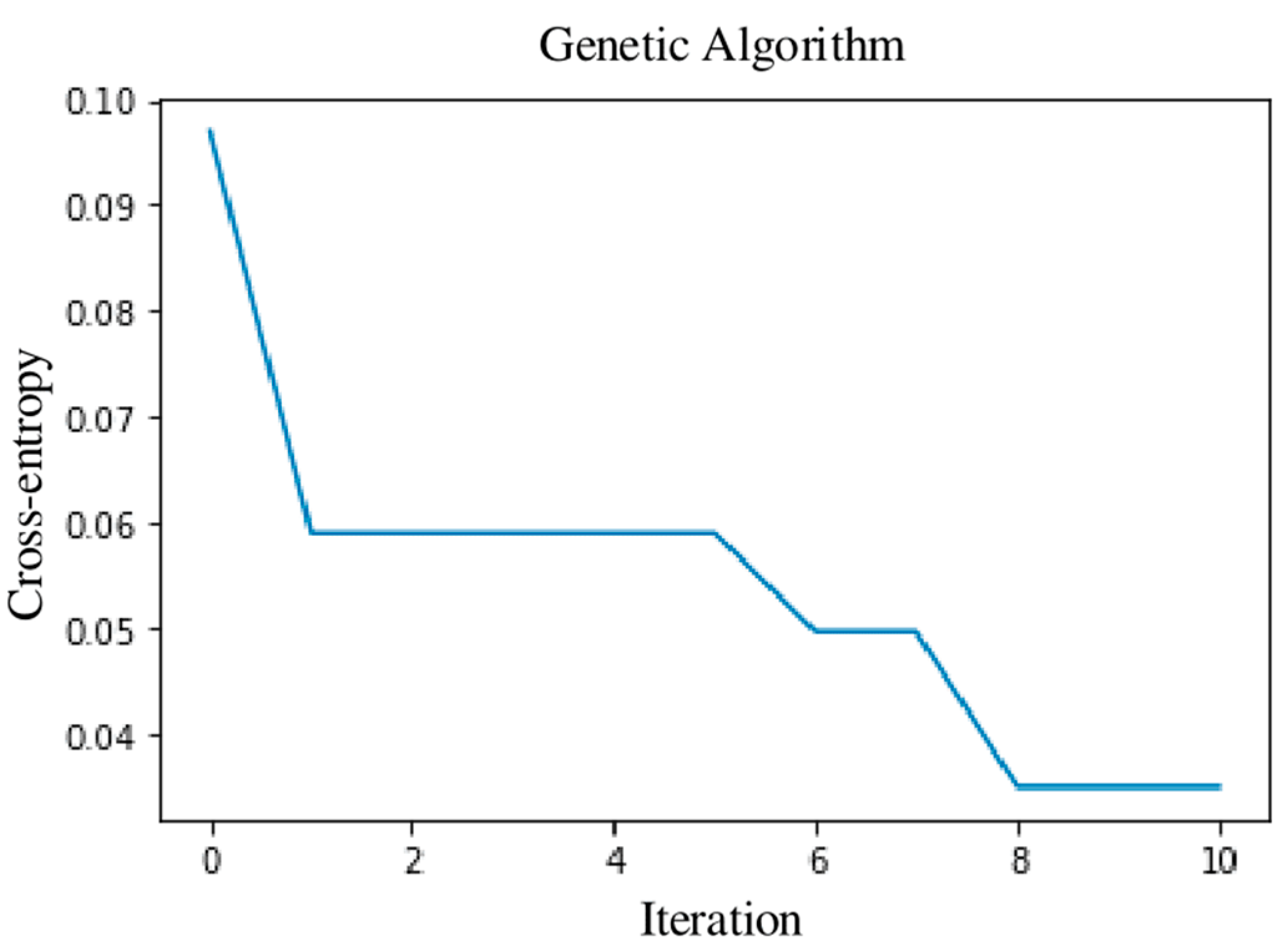
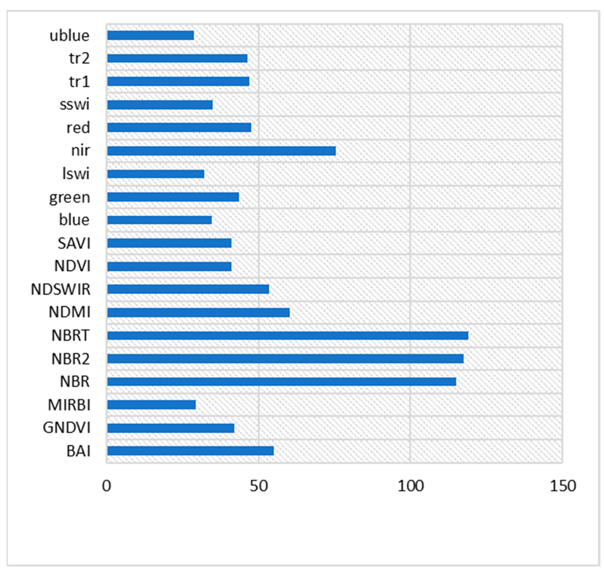
4.6. Genetic Algorithm (GA) for Optimal Features Selection
4.7. Resampling Reference Polygons
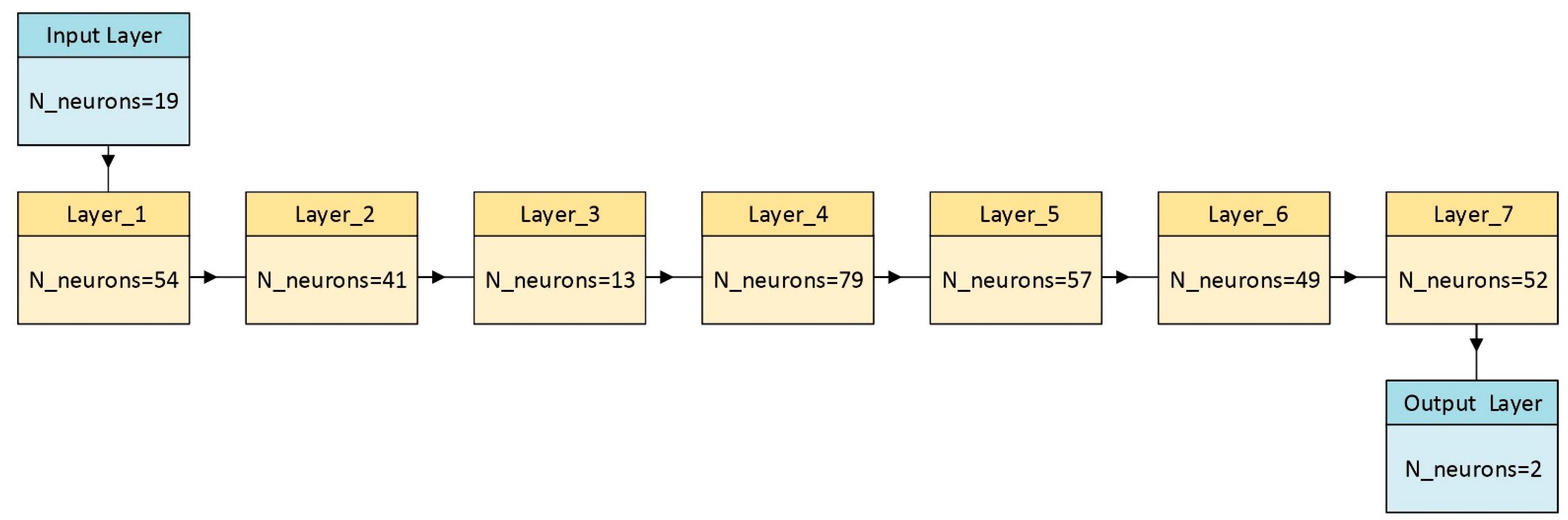
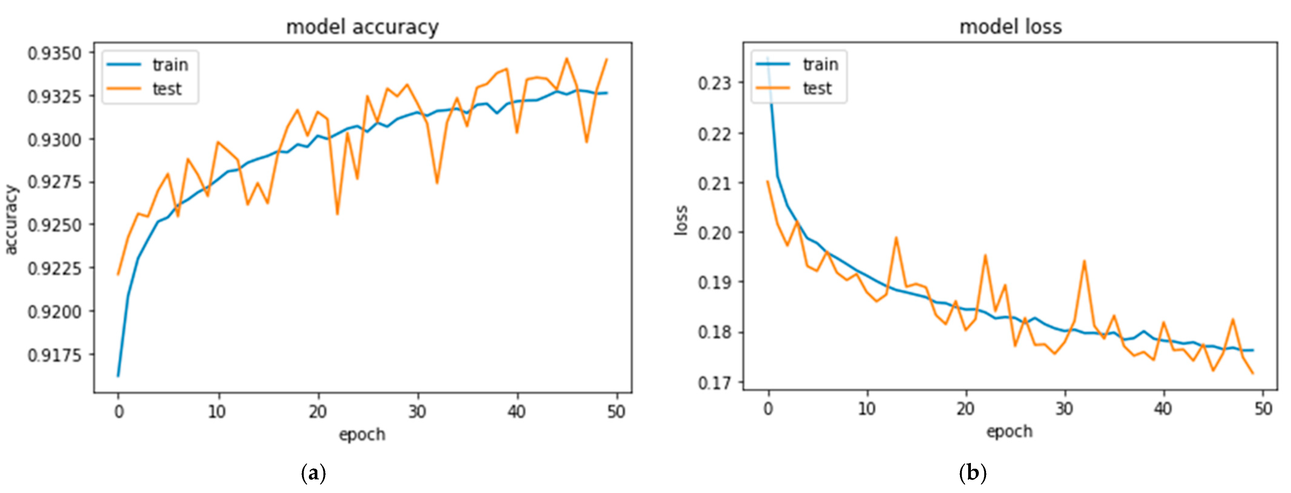
4.8. Neural Network (NN) Classifier
4.9. Random Forest (RF) Classifier
4.10. Accuracy Assessment and Performance Comparison
4.11. AccMODIS Direct Broadcast Burned Area Collection 6 (MCD64A1)
5. Results
5.1. Combination of Genetic Algorithm (GA) and Neural Network (NN) Classifiers
5.2. Random Forest (RF) Classifier
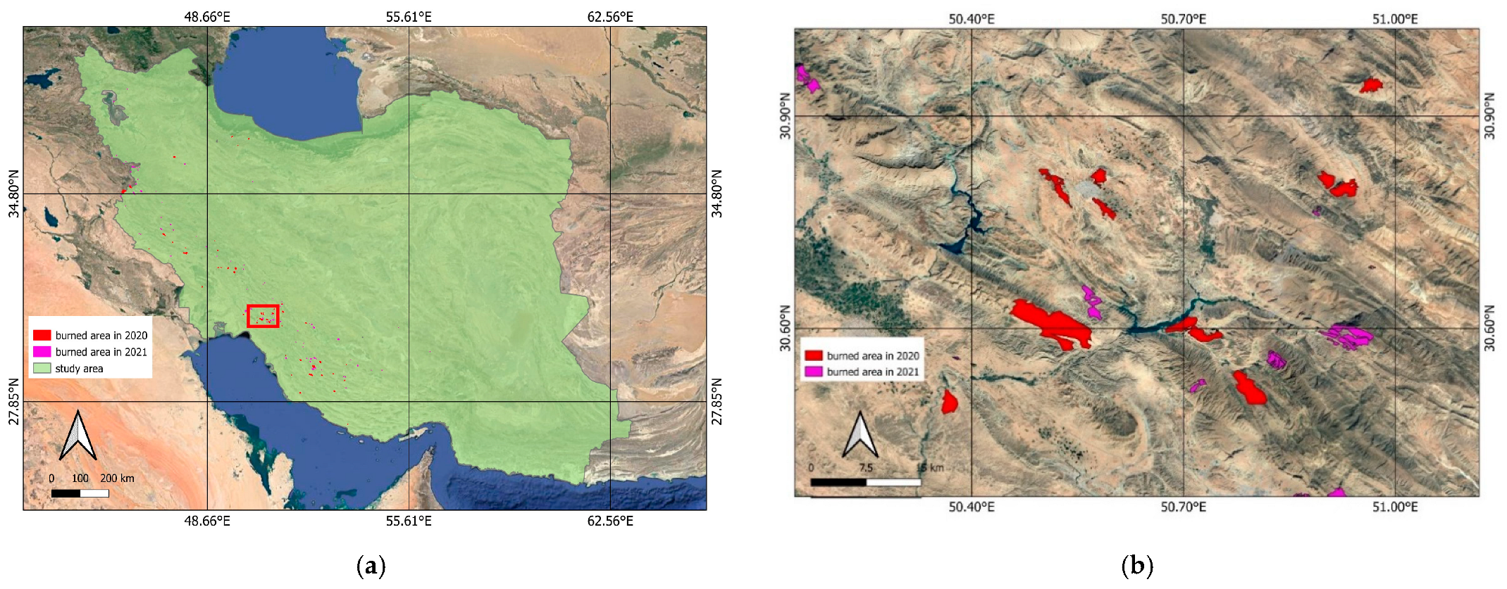
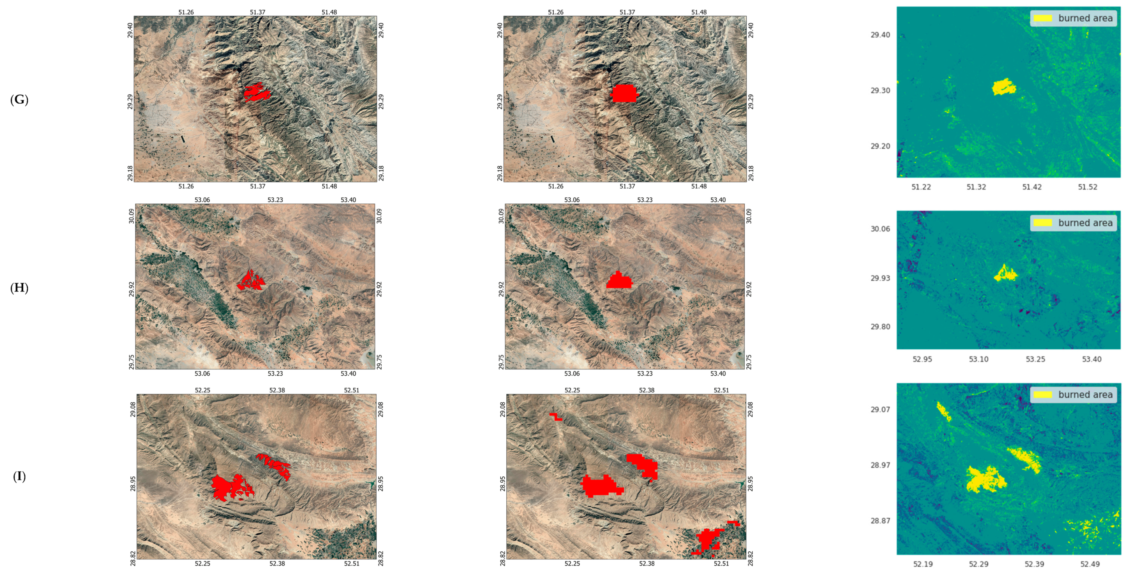
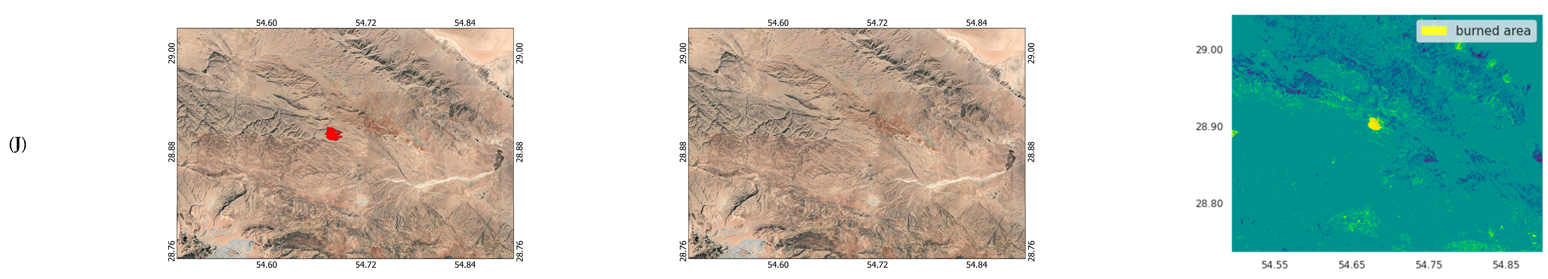
5.3. Validation
6. Discussion
7. Conclusions
Author Contributions
Funding
Data Availability Statement
Conflicts of Interest
References
- Liu, J.; Heiskanen, J.; Maeda, E.E.; Pellikka, P.K.E. Burned Area Detection Based on Landsat Time Series in Savannas of Southern Burkina Faso. Int. J. Appl. Earth Obs. Geoinf. 2018, 64, 210–220. [Google Scholar] [CrossRef] [Green Version]
- Bar, S.; Parida, B.R.; Pandey, A.C. Landsat-8 and Sentinel-2 Based Forest Fire Burn Area Mapping Using Machine Learning Algorithms on GEE Cloud Platform over Uttarakhand, Western Himalaya. Remote Sens. Appl. Soc. Environ. 2020, 18, 100324. [Google Scholar] [CrossRef]
- Ngadze, F.; Mpakairi, K.S.; Kavhu, B.; Ndaimani, H.; Maremba, M.S. Exploring the Utility of Sentinel-2 MSI and Landsat 8 OLI in Burned Area Mapping for a Heterogenous Savannah Landscape. PLoS ONE 2020, 15, e0232962. [Google Scholar] [CrossRef] [PubMed]
- Roteta, E.; Bastarrika, A.; Padilla, M.; Storm, T.; Chuvieco, E. Development of a Sentinel-2 Burned Area Algorithm: Generation of a Small Fire Database for Sub-Saharan Africa. Remote Sens. Environ. 2019, 222, 1–17. [Google Scholar] [CrossRef]
- Malambo, L.; Heatwole, C.D. Automated Training Sample Definition for Seasonal Burned Area Mapping. ISPRS J. Photogramm. Remote Sens. 2020, 160, 107–123. [Google Scholar] [CrossRef]
- Mallinis, G.; Mitsopoulos, I.; Chrysafi, I. Evaluating and Comparing Sentinel 2A and Landsat-8 Operational Land Imager (OLI) Spectral Indices for Estimating Fire Severity in a Mediterranean Pine Ecosystem of Greece. GIScience Remote Sens. 2018, 55, 1–18. [Google Scholar] [CrossRef]
- Filipponi, F. BAIS2: Burned Area Index for Sentinel-2. Proceedings 2018, 2, 364. [Google Scholar] [CrossRef] [Green Version]
- Hawbaker, T.J.; Vanderhoof, M.K.; Beal, Y.J.; Takacs, J.D.; Schmidt, G.L.; Falgout, J.T.; Williams, B.; Fairaux, N.M.; Caldwell, M.K.; Picotte, J.J.; et al. Mapping Burned Areas Using Dense Time-Series of Landsat Data. Remote Sens. Environ. 2017, 198, 504–522. [Google Scholar] [CrossRef]
- Cabral, A.I.R.; Silva, S.; Silva, P.C.; Vanneschi, L.; Vasconcelos, M.J. Burned Area Estimations Derived from Landsat ETM+ and OLI Data: Comparing Genetic Programming with Maximum Likelihood and Classification and Regression Trees. ISPRS J. Photogramm. Remote Sens. 2018, 142, 94–105. [Google Scholar] [CrossRef]
- García-Llamas, P.; Suárez-Seoane, S.; Fernández-Guisuraga, J.M.; Fernández-García, V.; Fernández-Manso, A.; Quintano, C.; Taboada, A.; Marcos, E.; Calvo, L. Evaluation and Comparison of Landsat 8, Sentinel-2 and Deimos-1 Remote Sensing Indices for Assessing Burn Severity in Mediterranean Fire-Prone Ecosystems. Int. J. Appl. Earth Obs. Geoinf. 2019, 80, 137–144. [Google Scholar] [CrossRef]
- Gómez, I.; Pilar Martín, M. Prototyping an Artificial Neural Network for Burned Area Mapping on a Regional Scale in Mediterranean Areas Using MODIS Images. Int. J. Appl. Earth Obs. Geoinf. 2011, 13, 741–752. [Google Scholar] [CrossRef]
- Navarro, G.; Caballero, I.; Silva, G.; Parra, P.C.; Vázquez, Á.; Caldeira, R. Evaluation of Forest Fire on Madeira Island Using Sentinel-2A MSI Imagery. Int. J. Appl. Earth Obs. Geoinf. 2017, 58, 97–106. [Google Scholar] [CrossRef] [Green Version]
- Teodoro, A.; Amaral, A. A Statistical and Spatial Analysis of Portuguese Forest Fires in Summer 2016 Considering Landsat 8 and Sentinel 2A Data. Environment 2019, 6, 36. [Google Scholar] [CrossRef] [Green Version]
- Arruda, V.L.S.; Piontekowski, V.J.; Alencar, A.; Pereira, R.S.; Matricardi, E.A.T. An Alternative Approach for Mapping Burn Scars Using Landsat Imagery, Google Earth Engine, and Deep Learning in the Brazilian Savanna. Remote Sens. Appl. Soc. Environ. 2021, 22, 100472. [Google Scholar] [CrossRef]
- Boschetti, L.; Roy, D.P.; Justice, C.O.; Humber, M.L. MODIS-Landsat Fusion for Large Area 30m Burned Area Mapping. Remote Sens. Environ. 2015, 161, 27–42. [Google Scholar] [CrossRef]
- Long, T.; Zhang, Z.; He, G.; Jiao, W.; Tang, C.; Wu, B.; Zhang, X.; Wang, G.; Yin, R. 30 m Resolution Global Annual Burned Area Mapping Based on Landsat Images and Google Earth Engine. Remote Sens. 2019, 11, 489. [Google Scholar] [CrossRef] [Green Version]
- Parks, S.A.; Holsinger, L.M.; Voss, M.A.; Loehman, R.A.; Robinson, N.P. Mean Composite Fire Severity Metrics Computed with Google Earth Engine Offer Improved Accuracy and Expanded Mapping Potential. Remote Sens. 2018, 10, 879. [Google Scholar] [CrossRef] [Green Version]
- Seydi, S.T.; Akhoondzadeh, M.; Amani, M.; Mahdavi, S. Wildfire Damage Assessment over Australia Using Sentinel-2 Imagery and Modis Land Cover Product within the Google Earth Engine Cloud Platform. Remote Sens. 2021, 13, 220. [Google Scholar] [CrossRef]
- Roy, D.P.; Huang, H.; Boschetti, L.; Giglio, L.; Yan, L.; Zhang, H.H.; Li, Z. Landsat-8 and Sentinel-2 Burned Area Mapping—A Combined Sensor Multi-Temporal Change Detection Approach. Remote Sens. Environ. 2019, 231, 111254. [Google Scholar] [CrossRef]
- Alencar, A.; Shimbo, J.Z.; Lenti, F.; Marques, C.B.; Zimbres, B.; Rosa, M.; Arruda, V.; Castro, I.; Ribeiro, J.P.F.M.; Varela, V.; et al. Mapping Three Decades of Changes in the Brazilian Savanna Native Vegetation Using Landsat Data Processed in the Google Earth Engine Platform. Remote Sens. 2020, 12, 924. [Google Scholar] [CrossRef]
- Cansler, C.A.; McKenzie, D. How Robust Are Burn Severity Indices When Applied in a New Region? Evaluation of Alternate Field-Based and Remote-Sensing Methods. Remote Sens. 2012, 4, 456–483. [Google Scholar] [CrossRef] [Green Version]
- Fang, L.; Yang, J.; Zu, J.; Li, G.; Zhang, J. Quantifying Influences and Relative Importance of Fire Weather, Topography, and Vegetation on Fire Size and Fire Severity in a Chinese Boreal Forest Landscape. For. Ecol. Manag. 2015, 356, 2–12. [Google Scholar] [CrossRef]
- Liu, S.; Zheng, Y.; Dalponte, M.; Tong, X. A Novel Fire Index-Based Burned Area Change Detection Approach Using Landsat-8 OLI Data. Eur. J. Remote Sens. 2020, 53, 104–112. [Google Scholar] [CrossRef] [Green Version]
- Quintero, N.; Viedma, O.; Urbieta, I.R.; Moreno, J.M. Assessing Landscape Fire Hazard by Multitemporal Automatic Classification of Landsat Time Series Using the Google Earth Engine in West-Central Spain. Forests 2019, 10, 518. [Google Scholar] [CrossRef] [Green Version]
- Mahdianpari, M.; Salehi, B.; Mohammadimanesh, F.; Homayouni, S.; Gill, E. The First Wetland Inventory Map of Newfoundland at a Spatial Resolution of 10 m Using Sentinel-1 and Sentinel-2 Data on the Google Earth Engine Cloud Computing Platform. Remote Sens. 2019, 11, 43. [Google Scholar] [CrossRef] [Green Version]
- Tassi, A.; Vizzari, M. Object-Oriented Lulc Classification in Google Earth Engine Combining Snic, Glcm, and Machine Learning Algorithms. Remote Sens. 2020, 12, 3776. [Google Scholar] [CrossRef]
- Liu, C.; Li, W.; Zhu, G.; Zhou, H.; Yan, H.; Xue, P. Land Use/Land Cover Changes and Their Driving Factors in the Northeastern Tibetan Plateau Based on Geographical Detectors and Google Earth Engine: A Case Study in Gannan Prefecture. Remote Sens. 2020, 12, 3139. [Google Scholar] [CrossRef]
- Praticò, S.; Solano, F.; Di Fazio, S.; Modica, G. Machine Learning Classification of Mediterranean Forest Habitats in Google Earth Engine Based on Seasonal Sentinel-2 Time-Series and Input Image Composition Optimisation. Remote Sens. 2021, 13, 586. [Google Scholar] [CrossRef]
- Stromann, O.; Nascetti, A.; Yousif, O.; Ban, Y. Dimensionality Reduction and Feature Selection for Object-Based Land Cover Classification Based on Sentinel-1 and Sentinel-2 Time Series Using Google Earth Engine. Remote Sens. 2020, 12, 76. [Google Scholar] [CrossRef] [Green Version]
- Ghaffarian, S.; Farhadabad, A.R.; Kerle, N. Post-Disaster Recovery Monitoring with Google Earth Engine. Appl. Sci. 2020, 10, 4574. [Google Scholar] [CrossRef]
- Noi Phan, T.; Kuch, V.; Lehnert, L.W. Land Cover Classification Using Google Earth Engine and Random Forest Classifier-the Role of Image Composition. Remote Sens. 2020, 12, 2411. [Google Scholar] [CrossRef]
- Qu, L.; Chen, Z.; Li, M.; Zhi, J.; Wang, H. Accuracy Improvements to Pixel-Based and Object-Based LULC Classification with Auxiliary Datasets from Google Earth Engine. Remote Sens. 2021, 13, 453. [Google Scholar] [CrossRef]
- Hu, Y.; Hu, Y. Land Cover Changes and Their Driving Mechanisms in Central Asia from 2001 to 2017 Supported by Google Earth Engine. Remote Sens. 2019, 11, 554. [Google Scholar] [CrossRef] [Green Version]
- Daldegan, G.A.; Roberts, D.A.; de Figueiredo Ribeiro, F. Spectral Mixture Analysis in Google Earth Engine to Model and Delineate Fire Scars over a Large Extent and a Long Time-Series in a Rainforest-Savanna Transition Zone. Remote Sens. Environ. 2019, 232, 111340. [Google Scholar] [CrossRef]
- Bright, B.C.; Hudak, A.T.; Kennedy, R.E.; Braaten, J.D.; Henareh Khalyani, A. Examining Post-Fire Vegetation Recovery with Landsat Time Series Analysis in Three Western North American Forest Types. Fire Ecol. 2019, 15, 8. [Google Scholar] [CrossRef] [Green Version]
- Hong, H.; Tsangaratos, P.; Ilia, I.; Liu, J.; Zhu, A.X.; Xu, C. Applying Genetic Algorithms to Set the Optimal Combination of Forest Fire Related Variables and Model Forest Fire Susceptibility Based on Data Mining Models. The Case of Dayu County, China. Sci. Total Environ. 2018, 630, 1044–1056. [Google Scholar] [CrossRef]
- Hawbaker, T.J.; Vanderhoof, M.K.; Schmidt, G.L.; Beal, Y.J.; Picotte, J.J.; Takacs, J.D.; Falgout, J.T.; Dwyer, J.L. The Landsat Burned Area Algorithm and Products for the Conterminous United States. Remote Sens. Environ. 2020, 244, 111801. [Google Scholar] [CrossRef]
- Ghorbanian, A.; Kakooei, M.; Amani, M.; Mahdavi, S.; Mohammadzadeh, A.; Hasanlou, M. Improved Land Cover Map of Iran Using Sentinel Imagery within Google Earth Engine and a Novel Automatic Workflow for Land Cover Classification Using Migrated Training Samples. ISPRS J. Photogramm. Remote Sens. 2020, 167, 276–288. [Google Scholar] [CrossRef]
- Jamali, A. Improving Land Use Land Cover Mapping of a Neural Network with Three Optimizers of Multi-Verse Optimizer, Genetic Algorithm, and Derivative-Free Function. Egypt. J. Remote Sens. Sp. Sci. 2021, 24, 373–390. [Google Scholar] [CrossRef]
- Fornacca, D.; Ren, G.; Xiao, W. Evaluating the Best Spectral Indices for the Detection of Burn Scars at Several Post-Fire Dates in a Mountainous Region of Northwest Yunnan, China. Remote Sens. 2018, 10, 1196. [Google Scholar] [CrossRef]
- Veraverbeke, S.; Harris, S.; Hook, S. Evaluating Spectral Indices for Burned Area Discrimination Using MODIS/ASTER (MASTER) Airborne Simulator Data. Remote Sens. Environ. 2011, 115, 2702–2709. [Google Scholar] [CrossRef]
- Wilson, E.H.; Sader, S.A. Detection of Forest Harvest Type Using Multiple Dates of Landsat TM Imagery. Remote Sens. Environ. 2002, 80, 385–396. [Google Scholar] [CrossRef]
- Huete, A.R. A Soil-Adjusted Vegetation Index (SAVI). Remote Sens. Environ. 1988, 25, 295–309. [Google Scholar] [CrossRef]
- Gerard, F.; Plummer, S.; Wadsworth, R.; Sanfeliu, A.F.; Iliffe, L.; Balzter, H.; Wyatt, B. Forest Fire Scar Detection in the Boreal Forest with Multitemporal SPOT-VEGETATION Data. IEEE Trans. Geosci. Remote Sens. 2003, 41, 2575–2585. [Google Scholar] [CrossRef]
- Gitelson, A.A.; Kaufman, Y.J.; Merzlyak, M.N. Use of a Green Channel in Remote Sensing of Global Vegetation from EOS-MODIS. Remote Sens. Environ. 1996, 58, 289–298. [Google Scholar] [CrossRef]
- Amani, M.; Ghorbanian, A.; Ahmadi, S.A.; Kakooei, M.; Moghimi, A.; Mirmazloumi, S.M.; Moghaddam, S.H.A.; Mahdavi, S.; Ghahremanloo, M.; Parsian, S.; et al. Google Earth Engine Cloud Computing Platform for Remote Sensing Big Data Applications: A Comprehensive Review. IEEE J. Sel. Top. Appl. Earth Obs. Remote Sens. 2020, 13, 5326–5350. [Google Scholar] [CrossRef]
- Zhang, D.D.; Zhang, L. Land Cover Change in the Central Region of the Lower Yangtze River Based on Landsat Imagery and the Google Earth Engine: A Case Study in Nanjing, China. Sensors 2020, 20, 2091. [Google Scholar] [CrossRef] [Green Version]
- Amani, M.; Kakooei, M.; Moghimi, A.; Ghorbanian, A.; Ranjgar, B.; Mahdavi, S.; Davidson, A.; Fisette, T.; Rollin, P.; Brisco, B.; et al. Application of Google Earth Engine Cloud Computing Platform, Sentinel Imagery, and Neural Networks for Crop Mapping in Canada. Remote Sens. 2020, 12, 3561. [Google Scholar] [CrossRef]
- Ebrahimy, H.; Aghighi, H.; Azadbakht, M.; Amani, M.; Mahdavi, S.; Matkan, A.A. Downscaling MODIS Land Surface Temperature Product Using an Adaptive Random Forest Regression Method and Google Earth Engine for a 19-Years Spatiotemporal Trend Analysis over Iran. IEEE J. Sel. Top. Appl. Earth Obs. Remote Sens. 2021, 14, 2103–2112. [Google Scholar] [CrossRef]
- Amani, M.; Mahdavi, S.; Afshar, M.; Brisco, B.; Huang, W.; Mirzadeh, S.M.J.; White, L.; Banks, S.; Montgomery, J.; Hopkinson, C. Canadian Wetland Inventory Using Google Earth Engine: The First Map and Preliminary Results. Remote Sens. 2019, 11, 842. [Google Scholar] [CrossRef]
- Aguirre-Gutiérrez, J.; Seijmonsbergen, A.C.; Duivenvoorden, J.F. Optimizing Land Cover Classification Accuracy for Change Detection, a Combined Pixel-Based and Object-Based Approach in a Mountainous Area in Mexico. Appl. Geogr. 2012, 34, 29–37. [Google Scholar] [CrossRef] [Green Version]
- Chughtai, A.H.; Abbasi, H.; Karas, I.R. A Review on Change Detection Method and Accuracy Assessment for Land Use Land Cover. Remote Sens. Appl. Soc. Environ. 2021, 22, 100482. [Google Scholar] [CrossRef]
- Panuju, D.R.; Paull, D.J.; Griffin, A.L. Change Detection Techniques Based on Multispectral Images for Investigating Land Cover Dynamics. Remote Sens. 2020, 12, 1781. [Google Scholar] [CrossRef]
- Sefrin, O.; Riese, F.M.; Keller, S. Deep Learning for Land Cover Change Detection. Remote Sens. 2021, 13, 78. [Google Scholar] [CrossRef]
- ZhiYong, L.; Liu, T.; Benediktsson, J.A.; Falco, N. Land Cover Change Detection Techniques: Very-High-Resolution Optical Images: A Review. IEEE Geosci. Remote Sens. Mag. 2022, 10, 44–63. [Google Scholar] [CrossRef]
- Amani, M.; Member, S.; Mahdavi, S.; Kakooei, M.; Ghorbanian, A.; Brisco, B.; Delancey, E.R.; Toure, S.; Reyes, E.L. Wetland Change Analysis in Alberta, Canada Using Four Decades of Landsat Imagery. IEEE J. Sel. Top. Appl. Earth Obs. Remote Sens. 2021, 14, 10314–10335. [Google Scholar] [CrossRef]
- Seydi, S.T.; Hasanlou, M. A New End-to-End Multi-Dimensional CNN Framework for Land Cover/Land Use Change Detection in Multi-Source Remote Sensing Datasets. Remote Sens. 2020, 12, 2010. [Google Scholar] [CrossRef]
- Amani, M.; Kakooei, M.; Ghorbanian, A.; Warren, R.; Mahdavi, S.; Brisco, B.; Moghimi, A.; Bourgeau-chavez, L.; Toure, S.; Paudel, A.; et al. Forty Years of Wetland Status and Trends Analyses in the Great Lakes Using Landsat Archive Imagery and Google Earth Engine. Remote Sens. 2022, 14, 3778. [Google Scholar] [CrossRef]
- Hasanlou, M.; Seydi, S.T. Hyperspectral Change Detection: An Experimental Comparative Study. Int. J. Remote Sens. 2018, 39, 7029–7083. [Google Scholar] [CrossRef]
- Sulova, A.; Arsanjani, J.J. Exploratory Analysis of Driving Force of Wildfires in Australia: An Application of Machine Learning within Google Earth Engine. Remote Sens. 2021, 13, 10. [Google Scholar] [CrossRef]
- Sheykhmousa, M.; Mahdianpari, M.; Ghanbari, H.; Mohammadimanesh, F.; Ghamisi, P.; Homayouni, S. Support Vector Machine Versus Random Forest for Remote Sensing Image Classification: A Meta-Analysis and Systematic Review. IEEE J. Sel. Top. Appl. Earth Obs. Remote Sens. 2020, 13, 6308–6325. [Google Scholar] [CrossRef]
- Ramo, R.; García, M.; Rodríguez, D.; Chuvieco, E. A Data Mining Approach for Global Burned Area Mapping. Int. J. Appl. Earth Obs. Geoinf. 2018, 73, 39–51. [Google Scholar] [CrossRef]
- Syifa, M.; Panahi, M.; Lee, C.W. Mapping of Post-Wildfire Burned Area Using a Hybrid Algorithm and Satellite Data: The Case of the Camp Fire Wildfire in California, USA. Remote Sens. 2020, 12, 623. [Google Scholar] [CrossRef] [Green Version]
- Mahdavi, S.; Salehi, B.; Amani, M.; Granger, J.; Brisco, B. A Dynamic Classi Fication Scheme for Mapping Spectrally Similar Classes: Application to Wetland Classification. Int. J. Appl. Earth Obs. Geoinf. 2019, 83, 101914. [Google Scholar] [CrossRef]
- Amani, M.; Salehi, B.; Mahdavi, S.; Brisco, B. A Multiple Classifier System to Improve Mapping Complex Land Covers: A Case Study of Wetland Classification Using SAR Data in Newfoundland, Canada. Int. J. Remote Sens. 2018, 39, 7370–7383. [Google Scholar] [CrossRef]
- Roteta, E.; Bastarrika, A.; Franquesa, M.; Chuvieco, E. Landsat and Sentinel-2 Based Burned Area Mapping Tools in Google Earth Engine. Remote Sens. 2021, 13, 816. [Google Scholar] [CrossRef]
- Pedergnana, M.; Marpu, P.R.; Mura, M.D.; Benediktsson, J.A.; Bruzzone, L. A Novel Technique for Optimal Feature Selection in Attribute Profiles Based on Genetic Algorithms. IEEE Trans. Geosci. Remote Sens. 2013, 51, 3514–3528. [Google Scholar] [CrossRef]
- Cai, J.; Luo, J.; Wang, S.; Yang, S. Feature Selection in Machine Learning: A New Perspective. Neurocomputing 2018, 300, 70–79. [Google Scholar] [CrossRef]
- Pal, M.; Foody, G.M. Feature Selection for Classification of Hyperspectral Data by SVM. IEEE Trans. Geosci. Remote Sens. 2010, 48, 2297–2307. [Google Scholar] [CrossRef] [Green Version]
- Tao, H.; Li, M.; Wang, M.; Lü, G. Annals of GIS Genetic Algorithm-Based Method for Forest Type Classification Using Multi-Temporal NDVI from Landsat TM Imagery. Ann. GIS 2019, 25, 33–43. [Google Scholar] [CrossRef]
- Celik, T. Change Detection in Satellite Images Using a Genetic Algorithm Approach. IEEE Geosci. Remote Sens. Lett. 2010, 7, 386–390. [Google Scholar] [CrossRef]
- Santos, F.; Dubovyk, O.; Menz, G. Monitoring Forest Dynamics in the Andean Amazon: The Applicability of Breakpoint Detection Methods Using Landsat Time-Series and Genetic Algorithms. Remote Sens. 2017, 9, 68. [Google Scholar] [CrossRef] [Green Version]
- Singh, A.; Singh, K.K. Satellite Image Classification Using Genetic Algorithm Trained Radial Basis Function Neural Network, Application to the Detection of Flooded Areas. J. Vis. Commun. Image Represent. 2017, 42, 173–182. [Google Scholar] [CrossRef]
- Ranjbar, S.; Zarei, A.; Hasanlou, M.; Akhoondzadeh, M.; Amini, J.; Amani, M. Machine Learning Inversion Approach for Soil Parameters Estimation over Vegetated Agricultural Areas Using a Combination of Water Cloud Model and Calibrated Integral Equation Model. J. Appl. Remote Sens. 2021, 15, 018503. [Google Scholar] [CrossRef]
- Loussaief, S.; Abdelkrim, A. Convolutional Neural Network Hyper-Parameters Optimization Based on Genetic Algorithms. Int. J. Adv. Comput. Sci. Appl. 2018, 9, 252–266. [Google Scholar] [CrossRef] [Green Version]
- De Alban, J.D.T.; Connette, G.M.; Oswald, P.; Webb, E.L. Combined Landsat and L-Band SAR Data Improves Land Cover Classification and Change Detection in Dynamic Tropical Landscapes. Remote Sens. 2018, 10, 306. [Google Scholar] [CrossRef] [Green Version]
- Ghorbanian, A.; Zaghian, S.; Asiyabi, R.M.; Amani, M.; Mohammadzadeh, A.; Jamali, S. Mangrove Ecosystem Mapping Using Sentinel-1 and Sentinel-2 Satellite Images and Random Forest Algorithm in Google Earth Engine. Remote Sens. 2021, 13, 2565. [Google Scholar] [CrossRef]
- Sokolova, M.; Lapalme, G. A Systematic Analysis of Performance Measures for Classification Tasks. Inf. Process. Manag. 2009, 45, 427–437. [Google Scholar] [CrossRef]
- Padilla, M.; Stehman, S.V.; Chuvieco, E. Validation of the 2008 MODIS-MCD45 Global Burned Area Product Using Stratified Random Sampling. Remote Sens. Environ. 2014, 144, 187–196. [Google Scholar] [CrossRef]
- McHugh, M.L. Lessons in Biostatistics Interrater Reliability: The Kappa Statistic. Biochem. Medica 2012, 22, 276–282. [Google Scholar] [CrossRef]
- Lasko, K. Incorporating Sentinel-1 SAR Imagery with the MODIS MCD64A1 Burned Area Product to Improve Burn Date Estimates and Reduce Burn Date Uncertainty in Wildland Fire Mapping. Geocarto Int. 2021, 36, 340–360. [Google Scholar] [CrossRef] [Green Version]
- Moreno Ruiz, J.A.; García Lázaro, J.R.; Del Águila Cano, I.; Leal, P.H. Burned Area Mapping in the North American Boreal Forest Using Terra-MODIS LTDR (2001-2011): A Comparison with the MCD45A1, MCD64A1 and BA GEOLAND-2 Products. Remote Sens. 2013, 6, 815–840. [Google Scholar] [CrossRef] [Green Version]
- Fornacca, D.; Ren, G.; Xiao, W. Performance of Three MODIS Fire Products (MCD45A1, MCD64A1, MCD14ML), and ESA Fire_CCI in a Mountainous Area of Northwest Yunnan, China, Characterized by Frequent Small Fires. Remote Sens. 2017, 9, 1131. [Google Scholar] [CrossRef]


| References | Equation | Abbreviation | Index Name |
|---|---|---|---|
| [8,40,41] | 1/((0.1 − Red)2 + (0.06 − NIR)2) | BAI | Burned Area Index |
| [8,40,41] | (10.0 × lSWIR) − (9.8 × sSWIR) + 2.0 | MIRBI | Mid InfraRed Burn Index |
| [8,40,41] | (NIR − lSWIR)/(NIR + lSWIR) | NBR | Normalized Burn Ratio |
| [8] | (sSWIR − lSWIR)/(sSWIR + lSWIR) | NRB2 | Normalized Burn Ratio 2 |
| [8,41] | (NIR − (lSWIR × tr1))/( NIR + (lSWIR × tr1)) | NBRT | Normalized Burn Ratio Thermal |
| [8,37,40,41] | (NIR − Red)/(NIR + Red) | NDVI | Normalized Difference Vegetation Index |
| [8,40,42] | (NIR − sSWIR)/(NIR + sSWIR) | NDMI | Normalized Difference Moisture Index |
| [8,41,43] | 1.5 × ((NIR − Red)/(NIR + Red + 0.5)) | SAVI | Soil-Adjusted Vegetation Index |
| [44] | (NIR − sSWIR)/(NIR + sSWIR) | NDSWIR | Normalized Difference SWIR |
| [40] | 1/(NIR − (0.05 × NIR))2 + (lSWIR − (0.2 × lSWIR)2) | BAIML | Burned Area Index |
| Modified–LSWIR | |||
| [40] | 0.2043 × Blue + 0.4158 × Green + 0.5524 × Red + 0.5741 × NIR + 0.3124 × sSWIR + 0.2303 × lSWIR | BRI | TassCap Brightness |
| [40] | −0.1603 × Blue − 0.2819 × Green − 0.4934 × Red + 0.794 × NIR − 0.0002 × sSWIR − 0.1446 × lSWIR | GRE | TassCap Greenness |
| [45] | (NIR/Green)/(NIR + Green) | GNDVI | Green normalized difference vegetation index |
| Parameter | Value |
|---|---|
| max_num_iteration | 10 |
| population_size | 100 |
| mutation_probability | 0.1 |
| elit_ratio | 0.01 |
| crossover_probability | 0.5 |
| parents_portion | 0.9 |
| crossover_type | uniform |
| max_iteration_without_improv | None |
| Optimal Indices | Optimal Bands |
|---|---|
| NBRT | Red |
| NBR2 | Green |
| NBR | Unblue |
| MIRBI | Blue |
| NDVI | NIR |
| NDMI | SWIR1 (sSWIR) |
| NDSWIR | SWIR2 (lSWIR) |
| GNDVI | Thermal Infrared 1 (tr1) |
| SAVI | Thermal Infrared 2 (tr2) |
| BAI |
| Optimizer | Adam |
|---|---|
| activation | relu |
| nLayers | 7 |
| nNeurons | [13,41,49,52,54,57,79] |
| Total of Test Data = 1444 | Unburned Class | Burned Class | NET | User Accuracy (%) | Commission Error (%) |
|---|---|---|---|---|---|
| Unburned class | 707 | 54 | 761 | 93 | 7 |
| Burned class | 33 | 650 | 683 | 95 | 5 |
| Total | 783 | 661 | Overall accuracy (%) = 94 Kappa coefficient (%) = 88 | ||
| Production accuracy (%) | 90 | 98 | |||
| Omission error (%) | 10 | 2 | |||
| Total of Test Data = 1444 | Unburned Class | Burned Class | NET | User Accuracy (%) | Commission Error (%) |
|---|---|---|---|---|---|
| Unburned class | 742 | 19 | 761 | 98 | 2 |
| Burned class | 41 | 642 | 683 | 94 | 6 |
| Total | 783 | 661 | Overall accuracy (%) = 96 Kappa coefficient (%) = 90 | ||
| Production accuracy (%) | 95 | 97 | |||
| Omission error (%) | 5 | 3 | |||
| ACC = TP + TN/(TP + FN + FP + TN) | Overall accuracy | 0.96 |
|---|---|---|
| TPR = TP/(TP + FN) | Sensitivity or recall | 0.97 |
| FPR = FP/(FP + TN) | Probability of false alarm | 0.06 |
| TNR = TN/(TN + FP) | Specificity | 0.94 |
| FNR = FN/(TP + FN) | Miss rate | 0.02 |
| PPV = TP/(TP + FP) | Precision | 0.95 |
| NPV = TN/(TN + FN) | Negative predictive value | 0.97 |
| FOR = FN/(FN + TN) | False omission rate | 0.03 |
| FDR = FP/(TP + FP) | False discovery rate | 0.05 |
Publisher’s Note: MDPI stays neutral with regard to jurisdictional claims in published maps and institutional affiliations. |
© 2022 by the authors. Licensee MDPI, Basel, Switzerland. This article is an open access article distributed under the terms and conditions of the Creative Commons Attribution (CC BY) license (https://creativecommons.org/licenses/by/4.0/).
Share and Cite
Gholamrezaie, H.; Hasanlou, M.; Amani, M.; Mirmazloumi, S.M. Automatic Mapping of Burned Areas Using Landsat 8 Time-Series Images in Google Earth Engine: A Case Study from Iran. Remote Sens. 2022, 14, 6376. https://doi.org/10.3390/rs14246376
Gholamrezaie H, Hasanlou M, Amani M, Mirmazloumi SM. Automatic Mapping of Burned Areas Using Landsat 8 Time-Series Images in Google Earth Engine: A Case Study from Iran. Remote Sensing. 2022; 14(24):6376. https://doi.org/10.3390/rs14246376
Chicago/Turabian StyleGholamrezaie, Houri, Mahdi Hasanlou, Meisam Amani, and S. Mohammad Mirmazloumi. 2022. "Automatic Mapping of Burned Areas Using Landsat 8 Time-Series Images in Google Earth Engine: A Case Study from Iran" Remote Sensing 14, no. 24: 6376. https://doi.org/10.3390/rs14246376