Abstract
High-resolution topographic and stratigraphic datasets have been increasing applied in active fault investigation and seismic hazard assessment. There is a need for the comprehensive analysis of active faults on the basis of the correlating geomorphologic features and stratigraphic data. The integration of TLS and GPR was adopted to characterize the 3D geometry of the fault on the Maoyaba segment of Litang fault. The TLS was used to obtain the high-resolution topographic data for establishing the 3D surficial model of the fault. The 2D 250 MHz and 500 MHz GPR profiles were carried out to image the shallow geometry of the fault along four survey lines. In addition, the 3D GPR survey was performed by ten 2D 500 MHz GPR profiles with 1 m spacing. From the 2D and 3D GPR results, a wedge-shaped deformation zone of the electromagnetic wave was clearly found on the GPR profiles, and it was considered to be the main fault zone with a small graben structure. Three faults were identified on the main fault zone, and fault F1 and F3 were the boundary faults, while the fault F2 was the secondary fault. The subsurface geometry of the fault on the GPR interpreted results is consistent with the geomorphologic features of the TLS-derived data, and it indicates that the Maoyaba fault is a typical, normal fault. For reducing the environmental disruption and economic losses, GPR was the most optimal method for detecting the subsurface structures of active faults in the Litang fault with a non-destructive and cost-effective fashion. The 3D surface and subsurface geometry of the fault was interpreted from the integrated data of TLS and GPR. The fusion data also offers the chance for the subsurface structures of active faults on the GPR profiles to be better understood with its corresponding superficial features. The study results demonstrate that the integration of TLS and GPR has the capability to obtain the high-resolution micro geomorphology and shallow geometry of active faults on the Maoyaba segment of the Litang fault, and it also provides a future prospect for the integration of TLS and GPR, and is valuable for active fault investigation and seismic hazard assessment, especially in the Qinghai-Tibet Plateau area.
1. Introduction
Geomorphic landforms and stratigraphic units commonly document the evidence of faulting caused by surface rupturing earthquakes. The evidence of faulting at the surface and shallow subsurface provides the useful information for constraining paleo-earthquake events, determining the fault slip rates and evaluating the seismic hazard [1,2,3,4,5,6,7]. In general, geomorphic evidence of faulting is identified and analyzed by the geomorphological markers from high-resolution topographic data, such as surface ruptures, fault scarps, fluvial terraces and so on [8,9,10,11,12,13]. The evidence of faulting in the shallow subsurface is correlated to the offsets of the stratigraphic units by trenching studies [14,15,16,17]. Thus, high-resolution topographic and stratigraphic datasets are crucial for active fault investigation and seismic hazard assessment.
Classical methods, such as the total station and RTK, were generally used to obtain high-resolution topographic data in a time-consuming and expensive way. To circumvent this, TLS has been typically adopted to acquire the high-resolution topographic data for describing the subtle geomorphologic features of active faults [18,19,20,21,22,23,24,25,26]. In addition, the subsurface structures of active faults were commonly revealed by trenching or borehole rather than the visual or optical inspection. In order to reduce environmental disruption and economic losses, the near-surface geophysics methods, including the electrical resistivity imaging, GPR and microgravimetry, were chosen to depict the shallow geometry in the vicinity of active faults [27,28,29,30]. In these methods, GPR was the most prominent method for imaging the subsurface structures of active faults with a non-destructive and cost-effective fashion [27,31,32,33,34,35,36]. Due to the electrical property contrasts in the different geological structures, the radar images were difficult to interpret without GPR survey experience, especially in complex geological environments. Therefore, it is valuable to conduct the integration of TLS and GPR for the comprehensive interpretation and analysis of active faults. 3D realistic surficial model and subsurface geometry of active faults can be characterized by the integrated data of TLS and GPR. The fusion data also offers the chance that the subsurface structures of active faults on the GPR profiles can be better understanding with its corresponding superficial features. Consequently, the integration of TLS and GPR has been widely applied in archaeology [37,38,39,40,41,42,43,44,45], building and road testing [46,47,48,49], geological survey [50,51,52,53,54,55,56,57,58,59], glacier detection [60] and other fields.
In recent years, the integration of TLS and GPR has been gradually applied in active faults investigation all over the world. Kayen. [50] used the TLS, GPR, and Spectral analysis of Surface Wave (SASW) to characterize the surface ruptures and shallow structure of the Denali fault. Spahic et al. [52] combined the TLS-derived data and GPR data to establish the 3D model of the outcrop wall using Gocad software. Schneiderwind. [56] provided the 3-D visualization method of paleo-seismic trench stratigraphy and logging by combining the T-LiDAR and GPR techniques. Bubek et al. [57] and Cowie. [58] integrated the TLS and GPR method to constrain the location of the hanging wall and the footwall for improving the vertical displacement of the normal fault. Although the integration of TLS and GPR has been used to obtain the high-resolution topographic data and shallow geometry of active faults in different geological environment all over the world, there were little the integration of TLS and GPR surveys had been performed on the Litang fault, especially in the Qinghai-Tibet Plateau area. Previous studies have different views on the motion mode of the Maoyaba fault as the followings: (1) the sinistral strike-slip fault with the thrust components [61]; (2) the normal fault with a vertical rate of 0.6 ± 0.1 mm/yr [62,63,64,65]. Furthermore, the Sichuan-Tibet railway will traverse the Maoyaba fault, so it is essential to study the motion mode of the Maoyaba fault in terms of the high-resolution topographic data and subsurface geometry. Owing to the severe natural environment in the southeastern Tibetan Plateau, the traditional methods were time-consuming and expensive to obtain the topographic data and shallow geometry of the Maoyaba fault.
In this study, the integration of TLS and GPR method was chosen to detect and reveal the 3D surface and subsurface geometry of the fault on the Maoyaba fault. After some preliminary geomorphologic investigations, TLS was used to provide 3D realistic surficial model of the fault, and the GPR survey with the 250 MHz and 500 MHz antenna was carried out to image the shallow geometry of the fault along the four survey lines. Moreover, ten 2D 500 MHz GPR profiles with 1 m spacing were realized to establish 3D GPR data for a better and reliable interpretation. The GPR data and the color point clouds were combined into a single dataset for the detailed 3D virtual reconstructions of the fault. The main objective of this study was to demonstrate the integration of TLS and GPR for delineating the 3D geometry of the fault on the Maoyaba fault, and it was also to reveal the motion mode of the Maoyaba fault on the basis of the correlating geomorphologic features and stratigraphic data.
2. Geological Setting
The Litang fault, situated in the southeast Tibetan Plateau with a low-relief, high-elevation (~4000–4500 m above the sea level) surface, is an important active fault for adjusting eastward extrusion of internal material in the Qinghai-Tibet Plateau (Figure 1a). It is approximately 190 km length and about 25 km width that starts from the northwest margin of Xiao Maoyaba Basin on the source of Wuliang river, traverses through the Maoyaba Basin, Litang Basin, Jiawa Basin, and terminates to the south of Dewu (Figure 1b) [61,65,66]. The Litang fault is a sinistral-lateral strike slip fault that mostly parallels to the left-lateral Xianshuihe fault (XSHF in Figure 1a) in eastern Tibetan Plateau, then gradually turning N-S. It has been highly active in the late Quaternary with several M ≥ 7 historical earthquakes including the 1886 M 7.1 earthquake occurred in the Maoyaba basin and the 1948 M 7.3 Litang earthquake with the surface ruptures distributed along the Litang and Jiawa-Dewu segments [64,67]. As a consequence, there are a series of hot springs, offset ridges, offset streams and surface ruptures along the Litang fault. The Litang fault is composed of four main segments, which are the Cuopu fault, the Maoyaba fault, the Litang fault and the Jiawa-Dewu fault from northwest to southeast, respectively (Figure 1b).
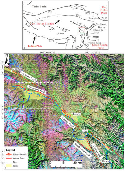
Figure 1.
Geometric distribution of the Litang fault. (a) Index maps of the west of China. The black arrows indicate the motion of the India plate relative to the Eurasian plane. The red rectangular box shows the Litang fault in Figure 1b. The black lines show the main active faults in the Tibetan plateau and the adjacent areas: LTF: Litang Fault; ATF: Altyn Tagh Fault; HYF: Haiyuan Fault; KLF: Kunlunshan Fault; GYF: Ganzi-Yushu Fault; XSHF: Xianshuihe Fault; ANHF: Anninghe Fault; ZMHF: Zemuhe Fault; XJF: Xiaojiang Fault; LMSF: Longmen Shan Fault; KKF: Karakoram Fault; GCF: Gyaring Co fault; BCF: Beng Co Fault; MFT: Main Frontal Thrust. (b) The Litang fault on the Landsat 7 satellite image. The Litang fault is a sinistral-lateral strike slip fault and it is composed of the Cuopu fault, the Maoyaba fault, the Litang fault and the Jiawa-Dewu fault. The white rectangular box represents the geometric distribution of the Maoyaba fault in Figure 2.
The Maoyaba fault is located in the northwestern section of Litang fault and it extends at least 55 km long with a nearly W-E striking (white rectangular box in Figure 1b). It is the main boundary fault almost along the north flank of the Maoyaba basin and it dominates the development of the Maoyaba basin. In fact, the Maoyaba basin consists of two asymmetrical sub-basins; and the western one is smaller than the eastern (Figure 2). In addition, the geomorphologic features are steep, with high mountains, and few rivers in the northern flank of the Maoyaba basin, while the southern side is almost flat with long rivers. The satellite image and field investigations also manifested that the active faults were mainly distributed along the northern edge of the Maoyaba basin rather than the southern. Previous studies have different views on the motion mode of the Maoyaba fault [61,62,63,64,65,66,67]. A series of well-developed fluvioglacial fans and fluvioglacial terraces with different ages were offset by the main fault. Many linear triangular facets and the fault scarps with the height of ~10–20 m were distinctly found along the northern margin of the Maoyaba basin. Moreover, a giant historical landslide (~0.64 × 10⁸–0.94 × 10⁸ m3) with an average sliding velocity of approximately 53.25 m/s is located in the northeast margin of Maoyaba basin (red polygon in Figure 2), which is known as the Luanshibao landslide [62,68,69]. The maximum sliding distance of the Luanshibao landslide is 3.83 km with an elevation drop of 820 m. Previous studies manifested that the Luanshibao landslide occurred at about 1980 ± 30a BP, and it may be caused by the ancient earthquake [70,71].The study site is located in the northeast of Heni village (30.23°N, 99.86°E) with ~4100 m high-elevation as showed in Figure 2, where about 60 km away from Litang city. From the Google Earth image and the panoramic image of the study site in Figure 3, the fault scarp offset terrace T1 and T2 are visible along the northern margin fault of the Maoyaba basin. Furthermore, the surface evidences of the main fault are clearly identified by the surface expression and geomorphologic features, and they all indicate that the Maoyaba fault has been highly active in the late Quaternary with the normal component. This study site provides a good opportunity to evaluate the integration of TLS and GPR for depicting the 3D surface and subsurface geometry of the fault on the Maoyaba fault.
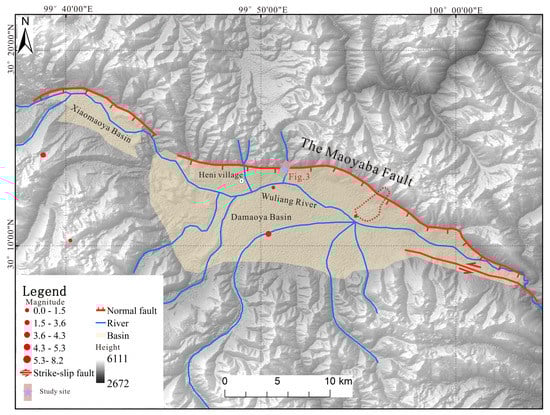
Figure 2.
Geometric distribution of the Maoyaba fault. The Maoyaba fault is the main boundary fault almost along the north flank of the Maoyaba basin (red lines). The red dots show the historical earthquakes. The rectangular box represents the survey site in Figure 3 and the red polygon indicates the location of the Luanshibao landslide.
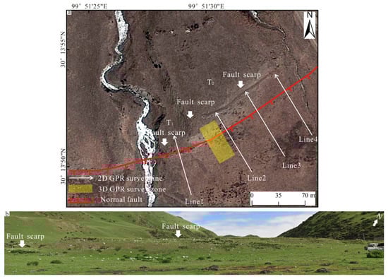
Figure 3.
Google Earth image and the panoramic image of the study site (the red rectangular box in Figure 2). (a) Google Earth image of the study site. Red lines represent the identified faults at the surface. White lines are the 2D 250 MHz and 500 MHz GPR survey lines. The yellow rectangular box indicates the 3D GPR survey zone. (b) The panoramic image of the study site.
3. Materials and Methods
3.1. TLS Data Acquisition and Processing
A Faro Focus3D X330 scanners was used to provide the high-resolution 3D model of the fault. This phase-shift scanner has the advantage of acquiring more density and precision data than the pulse-based laser scanner. It has an effective range of 330 m at 90% reflectivity and the resolution of the point clouds could reach 2 mm at a range of 25 m. The point clouds datasets were gathered with a horizontal view of 360° and a vertical view of 100°, and time consumption of one scanning station was about 12 min. In addition, the RGB information of point clouds was captured by an 8 M pix HDR camera into the scanner, and it could offer the texture maps for the point clouds.
The general sequence of TLS data acquisition includes the planning of the scanning stations, the location of the spherical reflector targets, scanning parameter settings and the geodetic coordinates of ground control points (GCP). In order to avoid possible omissions and ensure unabridged geomorphologic features of the fault, a total of 28 scanning stations were carried out with a distance between 30 to 50 m. At least three spherical reflector targets were placed into the overlap region of the adjacent scanning stations to combine all the point clouds into the same coordinates system. The GPS static measurement method was selected for gathering the geodetic coordinates of the GCPs with centimeter precision, and the spherical reflector targets were regarded as the GCPs in this study. Finally, the point clouds were transformed in a real word coordinate system by means of the geodetic coordinates of the GCPs. This provides the chance that TLS data can be merged with GPR data or other spatial data for comprehensive interpretation and analysis of active faults.
With the help of the spherical reflector targets, the point clouds were combined into a single set of point clouds datasets using Faro Scene software. In order to clearly show the surface model of point clouds datasets, filtering procedures were applied to eliminate the noise points using the Geomagic Studio software, such as vegetation, rocks, vehicles and people (Figure 4a). Generally, the most easily identifiable noise points (such as vehicles, people and the power lines) were manually removed in Geomagic Studio software within a 3D viewer. Then, the maximum local slope filter was used to suppress the unwanted laser returns, which were unable to be removed by the manual operation (Figure 4). After that, the point clouds resampling algorithm was conducted to reduce the amount of the point clouds datasets and retain the useful information.
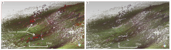
Figure 4.
The filter processing of the point clouds. (a) The raw point clouds. The point clouds were filtered using the Geomagic Studio software. Red points are the noise points, such as vegetation, rocks and vehicles and so on. (b) The filtering results of the point clouds.
3.2. GPR Data Acquisition and Processing
The GPR survey was performed to characterize the detailed subsurface geometry of the fault using a RAMAC system of MALA Geosciences (Figure 5). Data acquisition parameters were listed in Table 1. In this study, the 250 MHz and 500 MHz shielded antenna were chosen to optimize the sufficient penetration and proper spatial resolution [72]. The 250 MHz GPR antenna was employed to provide a general view of subsurface geometry of the fault along the four survey lines (white lines 1, 2, 3, 4 in Figure 3a), and the deformation zones on the GPR profiles were preliminarily distinguished by the distinctly variation of radar reflection waves. For revealing a better lateral and vertical resolution of the subsurface geometry, the deformation zones on the 250 MHz GPR profiles were scanned again by the 500 MHz GPR antenna. In view of the 250 MHz and 500 MHz GPR results, the 3D GPR investigation was carried out for depicting more detailed shallow geometry of the fault with a central frequency of 500 MHz (the yellow rectangular box in Figure 3a). A total of 10 parallel 2D 500 MHz GPR profiles were collected in the same direction with 1 m spacing.
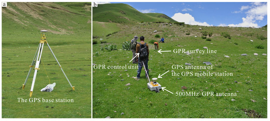
Figure 5.
The integrated system of GPR and the differential GPS. (a) The GPS base station. The GPS base station is often placed on a tripod, where located in the study site with a high elevation. (b) The integrated system of GPR and DGPS. The GPS antenna of the mobile station is situated on the middle-position of the GPR antenna. When the GPR antenna is pulled on the surface, the GPR data and the geographical coordinates are simultaneously obtained with the help of the pulse signals of the survey wheel.

Table 1.
Data acquisition parameters of the different GPR antennas.
In this work, the 250 MHz and 500 MHz profiles were conducted using a calibrated odometer fixed on the survey wheel. In order to determine the precise location of the subsurface structures, the integrated system of GPR and differential GPS (DGPS) was used to obtain the GPR data with geographical information (Figure 5). When the GPR antenna was pulled on the surface, the pulse signals of the survey wheel were applied to trigger the GPR control unit and the GPS signal receiver, respectively. Meanwhile, the GPR data and the geographical coordinates were simultaneously achieved by the GPR and the GPS signal receiver.
In general, there were many undesired signals or unwanted noises in the raw GPR data. In order to enhance the visual quality of the GPR signals and improve the data interpretation, different filters were essential to reduce the unwanted noises on the GPR raw data. In this study, the ReflexW 7.2 software was applied to process and interpret the GPR data. The general sequence was a relative standard procedure as shown in Figure 6. After optimizing and eliminating the invalid trace data in GPR raw data (Figure 6a), continuous or very low frequency components were decreased by the subtract-DC-shift filter (Figure 6b). The time zero correction was applied to refine the air/ground wavelength’s first time by the maximum amplitude peak of the trace, and the zero timing of 5.4 ns was performed in Figure 6c. Due to the electromagnetic energy will be weaken as the depth increases, the automatic gain control (AGC) was conducted to amplify the GPR signals using a mathematical function (Figure 6d). The signal reverberation and the horizontal reflections were suppressed by the background removal filter in Figure 6e. The band pass filter was used to remove the noise signals in GPR profile (Figure 6f), and the cut-off frequency of 150–450 MHz and 250–650 MHz were chosen to process the 250 MHz and 500 MHz GPR profiles. The running average filter was employed to suppress the background noises on the radar image and remove the antenna ringing signals (Figure 6g). The average electromagnetic wave velocity of ~0.08 m/ns was calculated using the time-to-depth conversation by the known depth. Finally, the topographic correction was conducted to compensate the two-way travel times in the vertical direction of the GPR data by the high-resolution topographic data (Figure 6h), which was recorded by the integrated GPR and DGPS system.
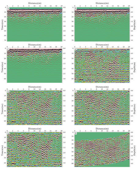
Figure 6.
The processing workflow of GPR data. (a) The raw GPR data. (b) subtract-DC-shift, (c) time-zero correction, (d) automatic gain control, (e) background removal, (f) band-pass filter, (g) running average filter, (h) topographic correction.
3.3. Data Integration Method of TLS and GPR
The TLS collects the dense point clouds with Cartesian coordinates (x, y, z) and texture maps to show the high resolution topographic data of active faults. The point clouds includes x, y, z coordinates of the scanning scene, the point attributes (such as the intensity value of the reflected laser beam) and the RGB images captured by the camera. GPR has been used to delineate the subsurface materials or buried-object on a gray or color 2D radar gram, which is composed of the continuous single channel reflection waves with the same trace interval. The subsurface materials or buried-object on the GPR image were identified by the variation in the pattern and relative amplitude of the electromagnetic waves.
Data integration workflow of TLS and GPR was described in Figure 7. First, the raw point clouds and the GPR data were both processed in the light of the data processing procedure illustrated in Section 3.1 and Section 3.2. With the help of the spherical reflector targets, the point clouds of the scanning stations were combined into a single set of point clouds datasets using the Faro Scene software. The filtering and re-sampled procedures were also used to reduce the amount of the point clouds datasets and retain the useful information by the Geomagic Studio software. To show the realistic geomorphologic features of the fault, the color point clouds were generated by the processed point clouds and the panoramic images. These color point clouds were transformed as the xyz feature in the geodetic coordinate system by means of the geodetic coordinates of the GCPs. Second, the GPR data and the geographical coordinates were simultaneously achieved by the pulse signals of the survey wheel on the GPR equipment, and the geographical information of GPR data was determined by the post-processed differential correction using a based station data or a reference station data. Furthermore, the time synchronization algorithm was proposed for data integration of GPR and DGPS, and each trace on the GPR profile had a well spatial correlation with the geographical coordinates of the GPS signal receiver. In view of the mathematical model of electromagnetic wave, the time depth conversion was implemented to each trace on the GPR profiles. Then the GPR data was converted into the point clouds datasets with xyz feature in the geodetic coordinate system, which was the same as the TLS point clouds. At last, once the TLS data and GPR data were geo-referenced in the same geodetic coordinate system, the subsurface data (GPR) should be integrated with the surface data (TLS) for comprehensive interpretation and analysis of the fault.
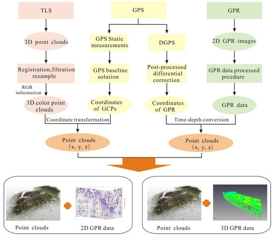
Figure 7.
Data integration method of TLS and GPR.
4. Results
4.1. Terrestrial Laser Scanning
The 3D color point clouds of the fault were shown in Figure 8a. Due to the limitation of vertical view, the blank areas indicate the location of the TLS scanning stations. It was difficult to identify the geomorphologic features of the fault on the point clouds. Compared with the point clouds, the digital elevation model (DEM) could provide the chance to qualitative and quantitative analysis for the morphologic features of the fault. In this study, the DEM was created by the filtered point clouds using the Delaunay triangulation in Geomagic Studio software (Figure 8b). The terrace T1 and T2 with nearly the W-E trending were apparently shown on the DEM. Moreover, the footwall and hanging wall of the fault and the surface ruptures were also clearly observed in Figure 8b. For the sake of showing more detailed geomorphologic features, an overlain map of the surface slope map and the topographic contours map with the contour intervals of 0.5 m were performed in ArcGIS software as shown in Figure 8c. There was a remarkable change in slope angle and the contour intervals across the fault, which is a good indication for the location of active faults. On the overlain map, the red areas were the exposed fault plane with the slope value of ~2243°. The hanging wall and footwall (the blue area) were both rather flat terrain with the lower slope (within 5°). In addition, the western portion of the fault plane was well preserved between the hanging wall and footwall. While the eastern portion might be affected by a human activities and there was a lower slope in the middle of the fault plane. The 3D surface model was established by the point clouds using the Golden Software Surfer 16 as shown in Figure 8d. A lower elevation area in the hanging wall, paralleling to active faults, was revealed on the 3D surface model (white polygon in Figure 8d). This implied that the hanging wall had been locally affected by later sedimentation.
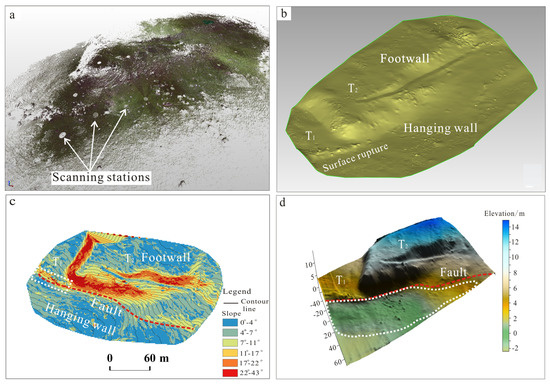
Figure 8.
TLS results. (a) The 3D color point clouds. (b) DEM. The fault offset terrace T1 and T2 with nearly the W-E trending are apparently described on the DEM. (c) The overlain map of the surface slope map and the topographic contours map. Red areas indicate the exposed fault plane with the slope values of ~22–43°, the blue areas show the flat terrain with the lower slope. Red lines represent active faults and black lines are the topographic contours. (d) 3D surface model of the fault. The white polygon represents the lower elevation area in the hanging wall.
4.2. Ground Penetrating Radar
4.2.1. 2D GPR Data
The topographic data of the GPR survey line (white line 1 in Figure 3a) was shown in Figure 9a, and there was an obvious topographic change at the horizontal distance of ~52 m. The maximum depth of ~7 m and 3 m were present on the processed 250 MHz and 500 MHz GPR profiles with SW-NE trending (Figure 9b,c). At the horizontal distance of ~52 m, the significantly variation in the waveform of the electromagnetic wave was observed on the 250 MHz and 500 MHz GPR images, especially in the 500 MHz GPR data. Compared with the high amplitude radar reflections, the reflection pattern of electromagnetic wave was dominantly by the low-amplitude radar reflections at a horizontal distance of ~52 m. The range of the low amplitude reflections area was visible from the surface to the bottom of the GPR image with a SE dipping. As a result, the interface of high amplitude radar reflections and low amplitude radar reflections at distance of ~52 m was supposed to be the fault F1 with a SE dipping, and it exhibited well consistency with the abrupt topographic changes on the surface as shown in Figure 9a,d (surface ruptures in the Figure 8b,c).
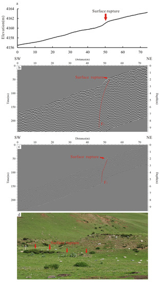
Figure 9.
The 250 MHz and 500 MHz GPR interpreted images. (a) show the topographic data of the GPR survey line 1. (b,c) show the processed 250 MHz and 500 MHz GPR profiles with SW-NE trending in the survey line 1. (d) show the surface ruptures on the GPR survey line 1.
The SW-NE trending profiles were performed to image the shallow geometry of the fault along the survey line 2 (Figure 10a,b). Between the horizontal distances of ~20 to 54 m, a wedge-shaped distortion and deformation zone was found on the processed 250 MHz and 500 MHz GPR profiles, especially in the 250 MHz GPR image. However, the reflection patterns of electromagnetic waves were different in the anomalous area. The middle portion of the anomalous area (~34 m) was characterized by the low-amplitude radar reflections, while the high amplitude reflections were exhibited at the two flanks of the deformation zone. At a distance of ~20–34 m, the deformation zone of electromagnetic waves was mainly dominated by high amplitude continuous horizontal reflections with relative regular waveforms, which associated to the homogeneous material in shallow subsurface. On the contrary, the right portion of the deformation zone (~34–54 m) was characterized by strong irregular or chaotic reflections attributed to the heterogeneous material. Therefore, the pronounced variations in the waveform and amplitude of the radar reflections were inferred as the fault plane at the GPR sections as shown in Figure 10a,b. The fault F1 and F3 were considered as the boundary fault, which was responsible for the development of the fault zone, whereas the F2 was the secondary fault in the fault zone.
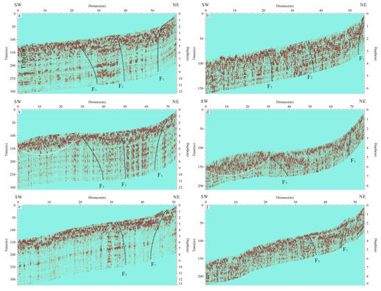
Figure 10.
The 250 MHz and 500 MHz GPR interpreted images. (a,b) show the 250 MHz and 500 MHz interpreted GPR results in the survey line 2. (c,d) show the 250 MHz and 500 MHz GPR images in the survey line 3 and (e,f) are the processed 250 MHz and 500 MHz GPR images in the survey line 4.
On the 250 MHz and 500 MHz GPR images along the measuring line 3 (Figure 3a), there were two obvious abnormal areas of electromagnetic waves at the horizontal distance of 0 to ~30 m and ~30 to 70 m (Figure 10c,d). At a distance of 0~30 m, the upmost part of 0 to ~1 m in depth was relative moderate amplitude reflections, while the high-amplitude continuous reflections related to the homogeneous material were displayed at the depth of ~1 to 2 m (white dash-dotted lines in Figure 10c,d). At a distance of ~30–70 m, a fault zone was observed by the remarkable changes of radar reflections on the 250 MHz and 500 MHz profiles, and the junctions of the high-amplitude and low-amplitude reflections at a distance of ~32 m, ~45 m and ~70 m were regarded as the fault plane, especially in the 250 MHz GPR image. In addition, the fault zone on the GPR data (Figure 10c,d) show a good consistency with the deformation zone on the 250 MHz and 500 MHz profile in Figure 10a,b, including the shallow geometry of the fault zone, the locations and the dipping of the fault plane. The GPR interpreted results were also proved by the GPR images along the survey line 4. The 250 MHz and 500 MHz GPR profiles (Figure 10e,f) were well aligned with the GPR data in Figure 10a–d (the fault F1 and F3). Due to the width of the fault zones lessening in survey line 4, the width of the fault zone on the surface was only ~15 m (Figure 10e,f) and it was narrower than the width of the deformation zone in Figure 8a,b and Figure 10c,d.
In view of the GPR results along the four survey lines, the wedge-shaped area between fault F1 and F3 was inferred as the main fault zone, and the maximum width on the surface could reach up to ~40 m. Moreover, the deformation zone on the GPR profiles was interpreted as a small graben structure by the geometry structure and the reflection pattern of electromagnetic waves, where a lower elevation area existed in the hanging wall of the fault (Figure 8d). Three faults were identified on the main fault zone as shown in Figure 10a–f. The fault F1 and F3 were a boundary fault and the fault F2 was the secondary fault in the fault zone. The fault F1 was supposed to be the main fault with a SE dipping and the fault F2 and were both tended to NE dipping. To sum up, the detailed shallow geometry of the fault at the depth of 0 to ~7 m were revealed by the 250 MHz and 500 MHz GPR profiles. The wedge-shaped deformation zone on the GPR data was deduced as a small garden structure and it indicated that the Maoyaba fault was a typical normal fault.
4.2.2. 3D GPR Data
The 3D GPR image was obtained by ten parallel 2D 500 MHz profiles, as shown in Figure 11 (the yellow rectangular box in Figure 3a). The 2D 500 MHz GPR profiles with the same trace interval of 1 m spacing were converted to the point clouds and displayed on the Bentley Pointools Software 1.5 (Figure 11a). The 3D GPR image was established by point clouds as shown in Figure 11b. In order to enhance the radar reflections contrasts, the GPR data was exhibited by the maximum amplitude values with a color map scale. As a consequence, the blue color on the GPR data indicated the deformation zone with the high-amplitude radar reflections, while the green color represented the low-amplitude radar reflections corresponding to the undesired or unwanted areas. Fault F1 and F2 were unambiguously distinguished at the boundaries of the high-amplitude radar reflections and low-amplitude radar reflections on the 3D GPR image (Figure 11). The interpreted results of the 3D GPR image were well aligned with the 2D GPR profiles in Figure 10a–d. Furthermore, the geomorphologic features of active faults on the surface were also further revealed by the 3D GPR data, such as the location of the fault plane, the striking, and dipping of the fault. Unfortunately, it is important to mention that fault F3 was not found on the 3D GPR image because of the limitation of the 3D GPR measuring lines. As a whole, the 3D GPR image had the chance to provide more detailed and realistic information for delineating the shallow geometry of the fault than the 2D GPR profile, and it played a vital role in identifying the subsurface structure of active faults on the GPR image. From the 3D GPR data, the wedge-shaped deformation zone between the fault F1 and F2 was clearly observed by the pronounced variations in the waveform and amplitude of the radar reflections. Furthermore, the characteristics of fault F1 and F2 were also directly confirmed on the 3D GPR data, such as the location of the fault plane, strikes, and dipping. Fault F1 was regarded as the main fault with a SE dipping of the nearly 90°, while fault F2 was the secondary fault in the fault zone with a NE dipping.
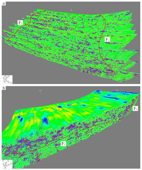
Figure 11.
3D GPR image. (a) show the 2D GPR profiles with the same trace interval of 1 m spacing. (b) indicates the 3D GPR image of the fault.
4.3. Data Visualization of Point Clouds and GPR Data
In view of the data integration method of TLS and GPR in Section 3.3, the GPR data (2D and 3D data) and the color point clouds were merged into a single dataset in Bentley Pointools Software 1.5 as displayed in Figure 12. Figure 12a,b show the data visualization of point clouds and 2D/3D GPR profiles. On the Figure 12b, the surface ruptures (white arrows) and fault F1 (red dotted line) were clearly observed on the fused data of point clouds and 2D GPR profiles, including the striking and the dipping of the fault. In addition, the topographic changes in the point clouds showed a good correlation with the location of the fault F1 on the GPR profile. To better interpret and understand the GPR data, the 3D surface and subsurface geometry of the fault were established by the integrated data of TLS and GPR as shown in Figure 12a,c. As a result, the integrated data of TLS and GPR rendered more the realistic surface and subsurface geometry of active faults, which not only allows discerning the fault traces at the surface (red dotted line in Figure 12a) and its strikes, but also obtain the range of the deformation zone and the location of fault dislocation. In addition, this hybrid data could offer the opportunity that the subsurface structures of the fault can be better understanding with its corresponding superficial data.
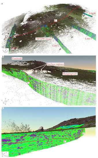
Figure 12.
Data visualization of point clouds and GPR profiles. (a,b) show data visualization of point clouds and 2D and 3D GPR profiles. (c) show data visualization of point clouds and 3D GPR profiles.
5. Discussion
5.1. The Integrated of TLS and GPR Method
Compared to single TLS or GPR method, the integration of TLS and GPR has the capability of detecting and identifying geomorphologic features and shallow geometry of active faults as the following: (1) the geomorphologic features and shallow geometry of active faults are simultaneously obtained by a non-destructive and cost-effective fashion; (2) multi-scale and multi-perspective spatial data are provided by the integration of TLS and GPR for imaging and analyzing the geomorphologic features and subsurface structures of active faults; (3) the 3D geometry of active faults can be established by the integrated data of TLS and GPR, and it also provides the chance that the shallow structures of the fault can be better understanding with its corresponding superficial data [50,52,56,57,58].
The TLS method has the capability of gaining the high-resolution topographic data and providing the detailed 3D virtual reconstructions of active faults. The fault offset T1 and T2 landscape with nearly the W-E trending and other geomorphic evidences of the faulting were apparently revealed on the TLS-derived data. A relative lower elevation area, paralleling to the fault, was well revealed on the TLS results and it implied that the hanging wall had been locally affected by later sedimentation (Figure 8d). In order to further verify the TLS results, the GPR system with the central frequencies of 250 MHz and 500 MHz were implemented to image the shallow geometry of active faults along the four survey lines (Figure 3a). The subsurface structures of the fault at the depth of ~7 m could be clearly shown on the 250 MHz and 500 MHz GPR processed profiles. In addition, a prominent abnormal zone of the electromagnetic waves was distinctly observed on the 250 MHz and 500 MHz GPR sections, especially in the survey lines 2 to 4 (Figure 10a–f). The radar reflections of the deformation zone were characterized by the remarkable variation in the waveform of the electromagnetic wave. On the GPR profiles in the survey lines 2 and 3 (Figure 10a–d), the width of the abnormal area could up to ~40 m at the surface and ~7m at the depth. However, the width of the fault zone on the surface was ~15 m in the survey lines 4, and it was narrower than the width of the deformation zone in Figure 10a–c,f. In view of the GPR results, the wedge-shaped anomalous area between fault F1 and F3 was inferred as the main fault zone and the maximum width on the surface could up to ~40 m (Figure 10a,c). Three faults were identified on the main fault zone as shown in Figure 10a–f. The fault F1 and F3 were the boundary fault and the fault F2 was the secondary fault in the fault zone. The GPR interpreted results associated to the subsurface geometry of fault was consistent with the geomorphologic features of the TLS-derived data. The wedge-shaped deformation zone on the GPR data was deduced as a small garden structure and it indicated that the Maoyaba fault was a typical normal fault.
Based on the data integration method of TLS and GPR, the GPR data and the color point clouds were combined into a single dataset for depicting the 3D surface and subsurface geometry of active faults. The study results demonstrate that the integration of TLS and GPR is suitable for delineating the 3D surface and subsurface geometry of the fault on the Maoyaba fault. Nevertheless, the integration of TLS and GPR was initially used to delineate the geomorphologic features and the subsurface geometry of the fault on the Maoyaba fault in this work. The application of the integration of TLS and GPR was still needed to further study in different geological environment. In particular, it is worth to pay a great attention to study the integration of GPR data and other spatial data for active faults investigation, such as the high-resolution remote sensing image, unmanned aerial vehicle, airborne LiDAR and so on.
5.2. The Maoyaba Fault
The remarkable geomorphic features of the late Quaternary in the Litang fault are numerous tectonic basins with NW, nearly EW and NNW striking, such as the Litang basin, Maoyaba basin and Jiawa basin. As the largest basin along the Litang fault, the Maoyaba basin is approximate diamond shape with nearly E-W striking, and it dominated by the Maoyaba fault. Zhou et.al. [73] suggested that the blocks between the Batang fault (a right-lateral strike-slip fault) and the Litang fault (a sinistral-lateral strike slip fault) slipped to south by the principal compressive stress with nearly EW directing, causing a nearly EW trending normal fault in the blocks, such as the Maoyaba fault. Based on the geomorphic features and morphology and tectonic of the basin, Ma et al. [62] illustrated that the Maoyaba basin is the rifted-basin, which is controlled by normal faults with nearly E-W striking, and the basin was formed from the nearly N-S trending extension and tension stress. The GPS data and focal mechanism analysis also confirmed that there was obvious tensional movement in the Litang-Batang area [71,74,75,76]. We concluded that the Maoyaba basin is a rifted-basin, which controlled by normal faults with nearly E-W striking. It is not a compressional fault basin as some researchers previously thought [61].
The Maoyaba fault, located in the northwestern section of the Litang fault, is the main boundary fault of the Maoyaba basin and it dominates the development of the Maoyaba basin. Satellite image and field investigations demonstrate that active faults are hander to follow on the south flank of the Maoyaba basin, and it indicates that the master fault is represented by the active fault along the northern edge of the Maoyaba basin. Numerous triangular facets are particularly impressive on the northern edge of the basin, which hints the normal component of the Maoyaba fault. In addition, the well-developed fault scarps cutting late Quaternary geomorphic features are well visible on the alluvial fans at the northern edge of the Maoyaba basin, and the steams or gullies flowing through the fault seem a plume spread at the base of the scarp [60,62,63,64,76]. This typical geomorphology show a well consistency with the normal motion of the Maoyaba fault, as well as the graben, horst and well-developed alluvio-glacial fans attest to the normal motion of the fault and its recent normal faulting activity. Owing to the severe natural environment on the Maoyaba fault, the traditional methods were time consuming and expensive to record the topographic data and shallow geometry of active faults. The integration of TLS and GPR was chosen to detect and reveal the 3D surface and subsurface geometry of the fault on the Maoyaba fault. Our study results show that the Maoyaba fault is characterized by normal fault activity in terms of tectonic geomorphology and shallow structure, so it should be a typical active normal fault, rather than a sinistral strike-slip fault with thrust components.
6. Conclusions
In this study, the integration of TLS and GPR was used to image the 3D surface and subsurface geometry of the Maoyaba fault, and also to reveal its motion mode. The conclusions associated to the study were described as the following:
- (1)
- The fault offset T1 and T2 landscape with nearly the W-E trending and other geomorphic evidences of faulting were revealed by the TLS-derived data. A relative lower elevation area, paralleling to the fault, was revealed on the TLS results and it implied that the hanging wall had been locally affected by later sedimentation.
- (2)
- On the 250 MHz and 500 MHz GPR profiles along the survey lines 2 to 4, a wedge-shaped zone of the electromagnetic wave was observed and it was considered as the main fault zone with a small graben structure, which the maximum width at the surface could up to ~40 m.
- (3)
- The characteristics of the fault F1 and F2 were directly confirmed on the 3D GPR data, such as the location of the fault plane, the strikes and dipping. The fault F1 was regarded as the main fault with a SE dipping of the nearly 90°, while the fault F2 was the secondary fault in the fault zone with a NE dipping.
- (4)
- The 3D surface and subsurface geometry of the fault were established by the integrated data of TLS and GPR. This hybrid data rendered more the realistic surface and subsurface geometry of active faults, which not only allows discerning the fault traces at the surface and its strikes, but also obtain the range of the deformation zone and the location of fault dislocation.
- (5)
- The study results demonstrate that integration of the TLS and GPR is suitable for delineating the 3D surface and subsurface geometry of the fault on the Maoyaba fault. In future research, the integration of TLS and GPR will be widely used for active fault investigation and seismic hazard assessment in different geological environments, especially in the Qinghai-Tibet Plateau area.
Author Contributions
Conceptualization, Z.W., methodology, D.Z., Z.W. and D.S., investigation, D.Z., Z.W. and J.L., writing—original draft preparation, D.Z., Z.W. and D.S., writing—review and editing, Z.W. and D.Z., software, Y.L., supervision, Z.W., project administration, D.Z., funding acquisition, D.Z. All authors have read and agreed to the published version of the manuscript.
Funding
This research was funded by Project funded by China Postdoctoral Science Foundation (No.2020M680606), Beijing Postdoctoral Research Foundation, the Science and Technique Foundation of Henan Province (No.222102320155, 22102210242) and the Key scientific research Foundation of the university in Henan Province (No.22A420003).
Data Availability Statement
The data presented in this study are available on request from the corresponding author.
Acknowledgments
We acknowledge support from the Chinese Geological Survey (DD20160268; DD20200319) of the Institute of Geomechanics, Chinese Academy of Geological Sciences for the Litang fault surveys in 2015 and 2020. We also thank Liu Jie for assistance with the field work and GPR data acquirement.
Conflicts of Interest
The authors declare no conflict of interest.
References
- Maruyama, T.; Lin, A. Active strike-slip faulting history inferred from offsets of topographic features and basement rocks: A case study of the Arima–Takatsuki Tectonic Line, southwest Japan. Tectonophysics 2002, 344, 81–101. [Google Scholar] [CrossRef]
- Hooper, D.M.; Bursik, M.I.; Webb, F.H. Application of high-resolution, interferometric DEMs to geomorphologic studies of fault scarps, Fish Lake Valley, Nevada-California, USA. Remote Sens. Environ. 2003, 84, 255–267. [Google Scholar] [CrossRef]
- Deng, Q.D.; Chen, L.C.; Ran, Y.K. Quantitative studies and applications of active tectonic. Earth Sci. Front. 2004, 11, 383–392. [Google Scholar]
- Arrowsmith, J.R.; Zielke, O. Tectonic geomorphology of the San Andreas Fault zone from high resolution topography: An example from the Cholame segment. Geomorphology 2009, 113, 70–81. [Google Scholar] [CrossRef]
- Liu, J.; Chen, T.; Zhang, P.Z.; Zhang, H.P.; Zheng, W.J.; Ren, Z.K.; Liang, S.M.; Sheng, C.Z.; Gan, W.J. Illuminating the active Haiyuan fault, China by Airborne Light Detection and Ranging. Chin. Sci. Bull. 2013, 58, 41–45. [Google Scholar]
- Ren, Z.K.; Zielke, O.; Yu, J.X. Active tectonics in 4D high-resolution. J. Struct. Geol. 2018, 117, 264–271. [Google Scholar] [CrossRef]
- Wu, Z.H. The Definition and Classification of Active faults: History, Current Status and Progress. Acta Geosci. Sin. 2019, 40, 661–697. [Google Scholar]
- Zhou, L.; Kaneda, H.; Mukoyama, S.; Nonomura, A.; Chibae, T. Detection of subtle tectonic–geomorphic features in densely forested mountains by very high-resolution airborne LiDAR survey. Geomorphology 2013, 182, 104–115. [Google Scholar]
- Chen, T.; Zhang, P.Z.; Liu, J.; Li, C.Y.; Ren, Z.K.; Hudnut, K.W. Quantitative study of tectonic geomorphology along Haiyuan fault based on airborne LiDAR. Chin. Sci. Bull. 2014, 59, 1293–1304. [Google Scholar] [CrossRef]
- Tang, Y. Measurement of the Spatial Scale of Fracture Dislocation through High-resolution Remote Sensing Images. China Earthq. Eng. J. 2019, 41, 1274–1279+1373. [Google Scholar]
- Wei, Z.Y.; He, H.L.; Su, P.; Zhuang, Q.T.; Sun, W. Investigating paleoseismicity using fault scarp morphology of the Dushanzi Reverse Fault in the northern Tian Shan, China. Geomorphology 2019, 327, 542–553. [Google Scholar] [CrossRef]
- Xiong, B.; Li, X. Offset measurements along active faults based on the structure from motion method-A case study of Gebiling in the Xorkoli section of the Altyn Tagh Fault. Sci. Technol. Eng. 2020, 20, 10848–10855. [Google Scholar] [CrossRef]
- Rao, G.; He, C.Q.; Chen, H.L.; Yang, X.P.; Shi, X.H.; Chen, P.; Hu, J.M.; Yao, Q.; Yang, C.J. Use of small unmanned aerial vehicle (sUAV)-acquired topography for identifying and characterizing active normal faults along the Seerteng Shan, North China. Geomorphology 2020, 359, 107168. [Google Scholar] [CrossRef]
- Ran, Y.K.; Deng, Q.D. History, status and trend about research of paleseismology. Chin. Sci. Bull. 1999, 44, 12–20. [Google Scholar] [CrossRef]
- Deng, Q.D. Advances and overview on researches of active tectonics in China. Geol. Rev. 2002, 18, 168–177. [Google Scholar]
- Wu, Z.H.; Zhang, Y.Q.; Hu, D.G. Neotectonics, active tectonics and earthquake geology. Geol. Bull. China 2014, 33, 391–402. [Google Scholar]
- Saint Fleur, N.; Klinger, Y.; Feuillet, N. Detailed map, displacement, paleoseismology, and segmentation of the Enriquillo-Plantain Garden Fault in Haiti. Tectonophysics 2020, 778, 228368. [Google Scholar] [CrossRef]
- Kayen, R.; Pack, R.T.; Bay, J.; Sugimoto, S.; Tanaka, H. Terrestrial-LIDAR Visualization of Surface and Structural Deformations of the 2004 Niigata Ken Chuetsu, Japan, Earthquake. Earthq. Spectra 2006, 22, 147–162. [Google Scholar] [CrossRef]
- Derron, M.H.; Jaboyedoff, M. Preface “LIDAR and DEM techniques for landslides monitoring and characterization”. Nat. Hazards Earth Syst. Sci. 2010, 10, 1877–1879. [Google Scholar] [CrossRef]
- Wei, Z.Y.; Shi, F.; Gao, X.; Xu, C.P.; He, H.L. Topographic characteristics of rupture associated with Wenchuan earthquake. Earth Sci. Front. 2010, 17, 53–66. [Google Scholar]
- Ma, H.C. Review on applications of LiDAR mapping technology to geosciences. Earth Sci. J. China Univ. Geosci. 2011, 36, 347–354. [Google Scholar]
- Gold, P.O.; Oskin, M.E.; Elliott, A.J.; Hinojosa-Corona, A.; Taylor, M.H.; Kreylos, O.; Cowgill, E. Coseismic slip variation assessed from terrestrial lidar scans of the El Mayor-Cucapah surface rupture. Earth Planet. Sci. Lett. 2013, 366, 151–162. [Google Scholar] [CrossRef]
- Ren, Z.K.; Chen, T.; Zhang, H.P.; Zheng, W.Z.; Zhang, P.Z. LiDAR Survey in Active Tectonics Studies:An Introduction and Overview. Acta Geol. Sin. 2014, 88, 1197–1202. [Google Scholar]
- Zheng, W.J.; Lei, Q.Y.; Du, P.; Chen, T.; Ren, Z.; Yu, J.X.; Zhang, N. 3D laser scanning (LiDAR): A new technology acquiring high precision palaeoearthquake trench information. Seismol. Geol. 2015, 37, 232–241. [Google Scholar]
- Tang, Y.Y.; Wei, S.Q.; Song, J.H.; Zhang, D.L.; Zheng, W.J. Key technology and application of terrestrial LiDAR in 3D active faults model. Acta Sci. Nat. Univ. Sunyatseni 2021, 60, 78–87. [Google Scholar]
- Zhang, D.; Li, J.C.; Wu, Z.H.; Liu, S.D.; Lu, Y. Using terrestrial LiDAR to accurately measure the microgeomorphologic geometry of active faults: A case study of fault scarp on the Maoyababa fault zone. J. Geomech. 2021, 27, 63–72. [Google Scholar]
- Carbonel, D.; Rodríguez-Tribaldos, V.; Gutiérrez, F.; Galve, J.P.; Guerrero, J.; Zarroca, M.; Roqué, C.; Linares, R.; McCalpin, J.P.; Acosta, E. Investigating a damaging buried sinkhole cluster in an urban area (Zaragoza city, NE Spain) integrating multiple techniques: Geomorphological surveys, DInSAR, DEMs, GPR, ERT, and trenching. Geomorphology 2015, 229, 3–16. [Google Scholar] [CrossRef]
- Wang, Z.P.; Liu, J.P.; Lei, Y.I. Effect and Application of 2D and 3D High Density Resistivity Method for Fault Detection. Sci. Technol. Eng. 2019, 19, 75–82. [Google Scholar]
- Nappi, R.; Paoletti, V.; D’Antonio, D.; Soldovieri, F.; Capozzoli, L.; Ludeno, G.; Porfido, S.; Michetti, A.M. Joint Interpretation of Geophysical Results and Geological Observations for Detecting Buried Active Faults: The Case of the “Il Lago” Plain (Pettoranello del Molise, Italy). Remote Sens. 2021, 13, 1555. [Google Scholar] [CrossRef]
- Finizola, A.; Ricci, T.; Deiana, R.; Cabusson, S.B.; Rossi, M.; Praticelli, N.; Giocoli, A.; Romano, G.; Delcher, E.; Suski, B.; et al. Adventive hydrothermal circulation on Stromboli volcano (Aeolian Islands, Italy) revealed by geophysical and geochemical approaches: Implications for general fluid flow models on volcanoes. J. Volcanol. Geotherm. Res. 2010, 196, 111–119. [Google Scholar] [CrossRef]
- Yalçıner, C.Ç.; Altunel, E.; Bano, M.; Meghraoui, M.; Karabacak, V.; Akyüz, H.S. Application of GPR to normal faults in the Buyuk Menderes Graben, western Turkey. J. Geodyn. 2013, 65, 218–227. [Google Scholar] [CrossRef]
- Dujardin, J.R.; Bano, M.; Schlupp, A.; Ferry, M.; Munkhuu, U.; Tsend-Ayush, N.; Enkhee, B. GPR measurements to assess the Emeelt active faults’s characteristics in a highly smooth topographic context, Mongolia. Geophys. J. Int. 2014, 198, 174–186. [Google Scholar] [CrossRef]
- Anchuela, Ó.P.; Lafuente, P.; Arlegui, L.; Liesa, C.L.; Simón, J.L. Geophysical characterization of buried active faults: The Concud Fault (Iberian Chain, NE Spain). Int. J. Earth Sci. 2016, 105, 2221–2239. [Google Scholar] [CrossRef]
- Zhang, D.; Li, J.C.; Wu, Z.H.; Ren, L.L. Review and application of ground penetrating radar in active faults. J. Geomech. 2016, 22, 733–746. [Google Scholar]
- Maurya, D.; Chowksey, V.; Tiwari, P.; Chamyal, L. Tectonic geomorphology and neotectonic setting of the seismically active South Wagad Fault (SWF), Western India, using field and GPR data. Acta Geophys. 2017, 65, 1167–1184. [Google Scholar] [CrossRef]
- Lunina, O.V.; Gladkov, A.S.; Gladkov, A.A. Surface and shallow subsurface structure of the Middle Kedrovaya paleoseismic rupture zone in the Baikal Mountains from geomorphological and ground-penetrating radar investigations. Geomorphology 2019, 326, 54–67. [Google Scholar] [CrossRef]
- Lubowiecka, L.; Armesto, J.; Arias, P.; Lorenzo, H. Historic bridge modelling using laser scanning, ground penetrating radar and finite element methods in the context of structural dynamics. Eng. Struct. 2009, 31, 2667–2676. [Google Scholar] [CrossRef]
- Solla, M.; Lorenzo, H.; Novo, A.; Riveiro, B. Evaluation of ancient structures by GPR (ground penetrating radar): The arch bridges of Galicia (Spain). Sci. Res. Essays 2011, 6, 1877–1884. [Google Scholar]
- Solla, M.; Lorenzo, H.; Rial, F.; Novo, A. Ground-penetrating radar for the structural evaluation of masonry bridges: Results and interpretational tools. Constr. Build. Mater. 2012, 29, 458–465. [Google Scholar] [CrossRef]
- Teixidó, T.; Peña, J.A.; Fernández, G.; Burillo, F.; Mostaza, T.; Zancajo, J. Ultradense topographic correction by 3D-laser scanning in pseudo-3D ground-penetrating radar data: Application to the constructive pattern of the monumental platform at the Segeda I Site (Spain). Archaeol. Prospect. 2014, 21, 113–123. [Google Scholar] [CrossRef]
- Zhao, W.K.; Forte, E.; Levi, S.T.; Pipan, M.; Tian, G. Improved high-resolution GPR imaging and characterization of prehistoric archaeological features by means of attribute analysis. J. Archaeol. Sci. 2015, 54, 77–85. [Google Scholar] [CrossRef]
- Aziz, A.S.; Stewart, R.R.; Green, S.L.; Flores, J.B. Locating and characterizing burials using 3D ground-penetrating radar (GPR) and terrestrial laser scanning (TLS) at the historic Mueschke Cemetery, Houston, Texas. J. Archaeol. Sci. Rep. 2016, 8, 392–405. [Google Scholar]
- Masini, N.; Capozzoli, L.; Chen, P.; Chen, F.; Romano, G.; Lu, P.; Tang, P.; Sileo, M.; Ge, Q.; Lasaponara, R. Towards an Operational Use of Geophysics for Archaeology in Henan (China): Methodological Approach and Results in Kaifeng. Remote Sens. 2017, 9, 809. [Google Scholar] [CrossRef]
- Puente, I.; Solla, M.; Lagüela, S.; Sanjurjo-Pinto, J. Reconstructing the Roman Site “Aquis Querquennis” (Bande, Spain) from GPR, T-LiDAR and IRT Data Fusion. Remote Sens. 2018, 10, 379. [Google Scholar] [CrossRef]
- Downs, C.; Rogers, J.; Collins, L.; Doering, T. Integrated Approach to Investigating Historic Cemeteries. Remote Sens. 2020, 12, 2690. [Google Scholar] [CrossRef]
- Solla, M.; Lorenzo, H.; Novo, A.; Caamaño, J.C. Structural analysis of the Roman Bibei bridge (Spain) based on GPR data and numerical modeling. Autom. Constr. 2012, 22, 334–339. [Google Scholar] [CrossRef]
- Puente, I.; Solla, M.; González-Jorge, H.; Arias, P. Validation of mobile LiDAR surveying for measuring pavement layer thicknesses and volumes. NDT E Int. 2013, 60, 70–76. [Google Scholar] [CrossRef]
- Lagüela, S.; Solla, M.; Puente, I.; Prego, F.J. Joint use of GPR, IRT and TLS techniques for the integral damage detection in paving. Constr. Build. Mater. 2018, 174, 749–760. [Google Scholar] [CrossRef]
- Pérez, J.P.C.; De Sanjosé Blasco, J.J.; Atkinson, A.D.J.; Del Río Pérez, L.M. Assessment of the Structural Integrity of the Roman Bridge of Alcántara (Spain) Using TLS and GPR. Remote Sens. 2018, 10, 387. [Google Scholar] [CrossRef]
- Kayen, R.; Barnhardt, A.; Carkin, B.A.; Grossman, E.E.; Minasian, D.; Thompson, M. Imaging the M7.9 Denali Fault Earthquake 2002 Rupture at the Delta River Using LiDAR, RADAR, and SASW Surface Wave Geophysics; AGU Fall Meeting: San Francisco, CA, USA, 2004. [Google Scholar]
- Lee, K.; Tomasso, M.; Ambrose, W.A.; Bouroullec, R. Integration of GPR with stratigraphic and lidar data to investigate behind-the-outcrop 3D geometry of a tidal channel reservoir analog, upper Ferron Sandstone, Utah. Lead. Edge 2007, 26, 929–1080. [Google Scholar] [CrossRef]
- Spahic, D.; Exner, U.; Behm, M.; Grasemann, B.; Haring, A. Structural 3D modeling using GPR in unconsolidated sediments (Vienna basin, Austria). Trabajos de Geología 2010, 30, 250–252, Erratum in Trabajos de Geología 2010, 29, 250–252. [Google Scholar]
- Aqeel, A.M. Measuring the Orientations of Hidden Subvertical Joints in Highways Rock Cuts Using Ground Penetrating Radar in Combination with LIDAR; Missouri University of Science and Technology: Rolla, MO, USA, 2012. [Google Scholar]
- Zhu, R.K.; Bai, B.; Yuan, X.J.; Luo, Z.; Wang, P.; Gao, Z.Y.; Su, L.; Li, T.T. A new approach for outcrop characterization and geostatistical analysis of meandering channels sandbodies within a delta plain setting using digital outcrop models: Upper triassic Yanchang tight sandstone formation, Yanhe outcrop, Ordos Basin. Acta Sedimentol. Sin. 2013, 31, 867–877. [Google Scholar]
- Maerz, N.H.; Aqeel, A.M.; Anderson, N. Measuring Orientations of Individual Concealed Sub-Vertical Discontinuities in Sandstone Rock Cuts Integrating Ground Penetrating Radar and Terrestrial LIDAR. Environ. Eng. Geosci. 2015, 21, 293–309. [Google Scholar] [CrossRef]
- Schneiderwind, S.; Mason, J.; Wiatr, T.; Papanikolaou, I.; Reicherter, K. 3-D visualisation of palaeoseismic trench stratigraphy and trench logging using terrestrial remote sensing and GPR—A multiparametric interpretation. Solid Earth 2016, 7, 323–340. [Google Scholar] [CrossRef]
- Bubeck, A.; Wilkinson, M.; Roberts, G.P.; Cowie, P.A.; McCaffrey, K.J.W.; Phillips, R.; Sammonds, P. The tectonic geomorphology of bedrock scarps on active normal faults in the Italian Apennines mapped using combined ground penetrating radar and terrestrial laser scanning. Geomorphology 2015, 237, 38–51. [Google Scholar] [CrossRef]
- Cowie, P.A.; Phillips, R.J.; Roberts, G.P.; McCaffrey, K.; Zijerveld, L.J.J.; Gregory, L.C.; Faure Walker, J.; Wedmore, L.N.J.; Dunai, T.J.; Binnie, S.A.; et al. Orogen-scale uplift in the central Italian Apennines drives episodic behaviour of earthquake faults. Sci. Rep. 2017, 7, 44858. [Google Scholar] [CrossRef]
- Zhang, D.; Wu, Z.H.; Li, C.Y.; Liu, S.T.; Ma, D.; Lu, Y. The delineation of three-dimensional shallow geometry of active fault based on TLS and GPR: A case study of an normal fault on the north margin of Maoyaba Basin in Litang, Western Sichuan Province. Seismol. Geol. 2019, 41, 377–399. [Google Scholar]
- Colucci, R.R.; Forte, E.; Boccali, C.; Dossi, M.; Lanza, L.; Pipan, M.; Guglielmin, M. Evaluation of Internal Structure, Volume and Mass of Glacial Bodies by Integrated LiDAR and Ground Penetrating Radar Surveys: The Case Study of Canin Eastern Glacieret (Julian Alps, Italy). Surv. Geophys. 2015, 36, 231–252. [Google Scholar] [CrossRef]
- Xu, X.W.; Wen, X.Z.; Yu, G.H.; Zheng, R.Z.; Luo, H.Y.; Zheng, B. Average slip rate, earthquake rupturing segmentation and recurrence behavior on the Litang fault zone, western Sichuan Province, China. Sci. China Ser. D Earth Sci. 2005, 48, 1183–1196. [Google Scholar] [CrossRef]
- Ma, D.; Wu, Z.H.; Li, J.C.; Li, Y.H.; Jiang, Y.; Liu, Y.H.; Zhou, C.J. Geometric Distribution and the Quaternary Activity of Litang Active Fault Zone Based on Remote Sensing. Acta Geol. Sin. 2014, 88, 1417–1435. [Google Scholar]
- Wu, Z.H.; Long, C.X.; Fan, T.Y.; Zhou, C.J.; Feng, H.; Yang, Z.Y.; Tong, Y.B. The arc rotational-shear active tectonic system on the southeastern margin of Tibetan Plateau and its dynamic characteristics and mechanism. Geol. Bull. China 2015, 34, 1–31. [Google Scholar]
- Chevalier, M.L.; Leloup, P.H.; Replumaz, A.; Pan, J.W.; Liu, D.L.; Li, H.B.; Gourbet, L.; Métois, M. Tectonic-geomorphology of the Litang fault system, SE Tibetan Plateau, and implication for regional seismic hazard. Tectonophysics 2016, 682, 278–292. [Google Scholar] [CrossRef]
- Zhou, C.J.; Wu, Z.H.; Zhang, K.Q.; Li, J.C.; Jiang, Y.; Tian, T.T.; Liu, Y.H.; Huang, X.J. New chronological constraint on the co-seismic surface rupture segments associated with the Litang Fault. Seismol. Geol. 2015, 37, 455–467. [Google Scholar]
- Zhou, R.J.; Chen, G.X.; Li, R.; Zhou, C.G.; Gong, Y.; He, Y.L.; Li, X.G. Study on Active Faults and Seismogenic Structure for the 1989 Batang M6.2~6.7 Earthquake Swarm in the Litang-Batang Region of West Sichuan,China %J Earthquake Research in China. Earthq. Res. China 2005, 3, 292–305. [Google Scholar]
- Zhang, Y.Z.; Replumaz, A.; Wang, G.C.; Leloup, P.H.; Gautheron, C.; Bernet, M.; Beek, P.V.D.; Paquette, J.L.; Wang, A.; Zhang, K.X.; et al. Timing and rate of exhumation along the Litang fault system, implication for fault reorganization in Southeast Tibet. Tectonics 2015, 34, 1219–1243. [Google Scholar] [CrossRef]
- Guo, C.B.; Zhang, Y.S.; Montgomery, D.R.; Du, Y.B.; Zhang, G.Z.; Wang, S.F. How unusual is the long-runout of the earthquake-triggered giant Luanshibao landslide, Tibetan Plateau, China? Geomorphology 2016, 259, 145–154. [Google Scholar] [CrossRef]
- Dai, Z.L.; Wang, F.W.; Cheng, Q.G.; Wang, Y.F.; Yang, H.F.; Lin, Q.W.; Yan, K.M.; Liu, F.C.; Li, K. A giant historical landslide on the eastern margin of the Tibetan Plateau. Bull. Eng. Geol. Environ. 2019, 78, 2055–2068. [Google Scholar] [CrossRef]
- Guo, C.B.; Du, Y.B.; Tong, Y.Q.; Zhang, Y.S.; Zhang, G.Z.; Zhang, M.; Ren, S.S. Huge long-runout landslide characteristics and for-mation mechanism: A case study of the Luanshibao landslide, Litang County, Tibetan Plateau. Geol. Bull. China 2016, 35, 1332–1345. [Google Scholar]
- Cao, Y.Y.; Huang, T.; Yin, X.K.; Zhou, P.H.; Xia, B. Shallow seismic explorations on unfavorable geological bodies in the Maoyaba basin of the Litang section of the Sichuan-Tibet railway. Prog. Geophys. 2022, 37, 774–785. [Google Scholar]
- Jol, H.M. Ground Penetrating Radar: Theory and Applications; Elsevier Science: Kidlington, UK, 2009. [Google Scholar]
- Zhou, R.J.; Chen, G.X.; Li, Y.; Zhou, C.H.; Gong, Y.; He, Y.L.; Li, X.G. Research on active faults in Litang-Batng region, Western Sichuan Province, and the seismogenic structures of the 1989 Batang M 6.7 earthquake swarm. Seismol. Geol. 2005, 27, 31–43. [Google Scholar]
- Li, Y.H.; Hao, M.; Ji, L.Y.; Qin, S.L. Fault slip rate and seismic moment deficit on major active faults in mid and south part of the Eastern margin of Tibet plateau. Chin. J. Geophys. 2014, 57, 1062–1078. [Google Scholar]
- Yin, G.X.; Long, F.; Liang, M.J.; Zhao, M.; Qi, Y.P.; Gong, Y.; Qiao, H.Z.; Wang, Z.; Wang, S.W.; Shui, L.R. Seismogenic structure of the M 4.9 and M5.1 Litang earthquakes on 23 September 2016 in southwestern China. Seismol. Geol. 2017, 39, 949–963. [Google Scholar]
- Zhao, B.; Gao, Y.; Liu, J.; Liang, S.S.; Xu, Z.G.; Du, G.B. Focal mechanism inversion and source depth locating of moderate-major b earthquakes in the Sichuan region since 2010. Chin. J. Geophys. 2019, 62, 130–142. [Google Scholar]


Publisher’s Note: MDPI stays neutral with regard to jurisdictional claims in published maps and institutional affiliations. |
© 2022 by the authors. Licensee MDPI, Basel, Switzerland. This article is an open access article distributed under the terms and conditions of the Creative Commons Attribution (CC BY) license (https://creativecommons.org/licenses/by/4.0/).