Abstract
On 2 January 2022, an earthquake of Ms 5.5 occurred in Ninglang County, Lijiang City, the earthquake-prone area of northwestern Yunnan. Whether this earthquake caused significant deformation and thermal anomalies and whether there is a relationship between them needs further investigation. Currently, multi-source remote sensing technology has become a powerful tool for long-time-series monitoring of earthquakes and active ruptures which mainly focuses on single crustal deformation and thermal anomaly. This study aims to reveal the crustal deformation and thermal anomaly characteristics of the Ninglang earthquake by using both Interferometric Synthetic Aperture Radar (InSAR) and Robust Satellite Techniques (RST). First, Sentinel-1A satellite SAR data were selected to obtain the coseismic deformation field based on Differential InSAR (D-InSAR), and the Small Baseline Set InSAR (SBAS-InSAR) technique was exploited to invert the pre- and post-earthquake displacement sequences. Then, RST was used to extract the thermal anomalies before and after the earthquake by using Moderate Resolution Imaging Spectroradiometer Land Surface Temperature (MODIS LST). The results indicate that the seismic crustal deformation is dominated by subsidence, with 23 thermal anomalies before and after the earthquake. It is speculated that the Yongning Fault in the deformation area is the main seismogenic fault of the Ninglang earthquake, which is dominated by positive fault dip-slip motion. Meanwhile, the seismic fault system composed of NE- and NW-oriented faults is an important factor in the formation of thermal anomalies, which are accompanied by changes in stress at different stages before and after the earthquake. Moreover, the crustal deformation and seismic thermal anomalies are correlated in time and space, and the active rupture activities in the region produce deformation accompanied by changes in thermal radiation. This study provides clues from remote sensing observations for analyzing the Ninglang earthquake and provides a reference for the joint application of InSAR and RST for earthquake monitoring.
1. Introduction
The distribution of seismic zones, the occurrence of moderate to strong earthquakes, and regional tectonic activities are all related to active ruptures []. The crustal motion of active fractures is long and slow, producing deformation with changes in geophysical fields such as thermal radiation. Earthquakes, as a local part of the rupture activity cycle, are brief and sudden tectonic events in the long-term activity of active ruptures. China is a country with serious seismic hazards. In particular, the geologically complex Sichuan–Yunnan region involves dense active fractures [], and medium to strong earthquakes are frequent in this region. It is difficult to obtain timely earthquake information with traditional seismic monitoring methods. In the early 1970s, remote sensing was first used for investigating seismic activity rupture and tectonic geomorphology []. With the development of remote sensing technology, various satellite sensors such as optical, thermal infrared, and microwave are applied for earth observation. Meanwhile, a large amount of remote sensing image data (multi-temporal, multi-spectral, multi-sensor, multi-platform, and multi-resolution) can be acquired for the same area. Hence, remote sensing technology has been extensively used in the field of seismotectonics [], including studies on active ruptures and tectonic landforms in seismic zones [,,,], crustal deformation [,,,,,,], pre- and post-earthquake thermal anomalies [,,,,,], pre-earthquake gas and aerosol changes [,,,], etc.
Interferometric Synthetic Aperture Radar (InSAR) has the characteristics of full-time, all-weather, high-accuracy, and wide-area coverage. It is widely used to measure the coseismic deformation, interseismic deformation, and postseismic deformation of earthquakes. The Differential InSAR (D-InSAR) technique was first used to measure the coseismic deformation of the 1992 Landers earthquake in California, USA, in 1993 []. Later, hundreds of earthquakes worldwide were studied by using D-InSAR [,,,,,,]. In recent years, D-InSAR deformation monitoring results have become the primary data source for seismic monitoring and source inversion []. However, the D-InSAR technique is limited by temporal and spatial decoherence in dense vegetation-covered areas. To address this issue, time series InSAR was born, and a series of advanced algorithms were proposed, such as Small Baseline Set InSAR (SBAS-InSAR) [] and Persistent Scatterer InSAR (PS-InSAR) []. The temporal InSAR technique has been used for interseismic slow deformation monitoring of active ruptures such as the Altyn Tagh Fault [,,,,], the Haiyuan Fault [,,], the Xianshui River Fault [], and the North Anatolian Fault [,] in Turkey. SBAS-InSAR selects multi-dominant interferograms with shorter spatio-temporal baselines, which can overcome the effects of spatio-temporal decoherence and atmospheric delay better than PS-InSAR [,].
Thermal infrared remote sensing uses satellite-based or airborne sensors to collect and record thermal infrared information of features. Polar-orbiting sun-synchronous satellites can obtain global observations every one or two days. Therefore, thermal infrared remote sensing can be exploited to monitor earthquake-prone areas and obtain information on surface temperature changes associated with impending earthquakes. In 1988, Gorny et al. pointed out that short-lived thermal infrared radiation enhancements precede many moderate-to-strong earthquakes at fault intersections in the seismically active areas of Central Asia []. Based on this, the idea that satellite thermal infrared can predict earthquakes was first proposed. The extraction of seismic thermal anomaly information using remote sensing has evolved from the initial visual judgment to fusing multiple parameters and methods, including Robust Satellite Techniques (RST), wavelet analysis, vorticity algorithms, power spectrum, and many other methods. Among them, the RST [] proposed by Tramutoli et al. uses long time series of satellite data to construct a normal background of the signal and uses the Gaussian distribution characteristics of remote sensing data values to extract the deviation degree relative to the background field. RST has been used to detect spatial and temporal thermal anomalies on the Earth’s surface recorded by satellites months to weeks before the occurrence of several earthquakes in China, Greece, Italy, and India [,,,,,,], for example.
Studying the crustal deformation and thermal anomaly characteristics of active ruptures in seismic regions and their change processes with rupture activities helps to further understand tectonic activities. Meanwhile, combining thermal infrared and radar remote sensing observations can obtain information on regional tectonic deformation and the strength of fault activity, as well as clues to find active ruptures [].
According to the China Earthquake Network Center (CENC), on 2 January 2022, at 15:02 (GMT + 8), an Ms 5.5 earthquake with a source depth of 10 km occurred in Ninglang County, Lijiang City, Yunnan Province, southwestern China (27.79°N, 100.65°E, Table 1). The macroscopic epicenter of the earthquake was in the area of Zhongwadu, Shangwadu, and Gala of Yongning Village, Yongning Town, 60 km from Ninglang County and 64 km from Muli County, Sichuan Province. The following earthquakes of Ms 3.4, Ms 4.6, Ms 4.1, and Ms 4.2 occurred in the area on 6 April, 16, 17 and 30 April. There is no clear answer to whether the Ninglang earthquake caused significant deformation and thermal anomalies and the relationship between them, and in-depth investigations are needed.

Table 1.
The focal mechanism solutions of the Ninglang earthquake on 2 January 2022 given by different institutions. (Institute of Geophysics of the China Earthquake Administration, IGP-CEA []; Global Centroid-Moment-Tensor, GCMT []; United States Geological Survey, USGS []; Helmholtz Centre Potsdam—German Research Centre for Geosciences, GFZ []).
In this study, the InSAR technique was combined with RST. The ascending and descending Sentinel-1A SAR data (the range is shown in Figure 1) and the nighttime Moderate Resolution Imaging Spectroradiometer Land Surface Temperature (MODIS LST) data were selected. From this data, the coseismic deformation field of the 2022 Ninglang Ms 5.5 earthquake was obtained by D-InSAR, and the crustal deformation before and after the earthquake was obtained by SBAS-InSAR. Meanwhile, the thermal anomalies before and after the earthquake were extracted by RST. Then, combined with the regional geotectonic background and the solution of the seismic mechanism from related institutions, the coupling relationship between the InSAR crustal deformation and seismic thermal anomalies of the Ninglang earthquake was investigated. Finally, the macroscopic epicenter location, coseismic characteristics, and possible seismogenic ruptures of the 2022 Ninglang earthquake were further revealed.
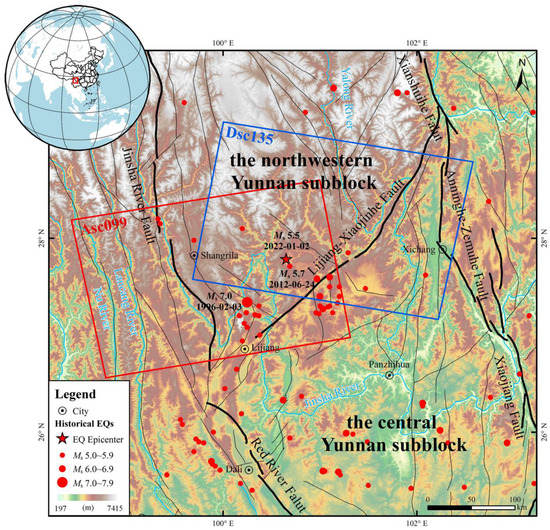
Figure 1.
The historical earthquake distribution map of the northwestern Yunnan subblock to the central Yunnan subblock and neighboring areas. The faults are based on the “Active Tectonic Map of China (1:4 million)” []. Historical earthquakes are from CENC’s catalogue of earthquakes greater than 5.0 magnitude from 1970 to the present. The base map is NASADEM from Earthdata [].
2. Geological and Tectonic Background
The Ninglang area of Lijiang, China, is located in the middle of the Sichuan–Yunnan rhombic block, in the southwest section of the Lijiang–Xiaojinhe Fault. Due to the collision and subduction of the Indo-Eurasian plate, a large amount of material from the southeastern margin of the Tibetan Plateau escaped in the southeastern direction, and the Sichuan–Yunnan region rotated clockwise around the Himalayan East tectonic knot, forming the current tectonic pattern of the Sichuan–Yunnan rhombic block [,,,,]. The complex interlocking geological formations, strong crustal deformation, and fracture activities cause moderate to strong earthquakes to occur frequently in the Ninglang area of Lijiang, and this area is known as the “earthquake nest” [,]. According to the historical earthquake catalog of the CENC (from 1970 to present), the southwest section of the Lijiang–Xiaojinhe Fault (Lijiang–Ninglang section) is more seismically active than the northeast section, with 23 earthquakes of Ms 5.0 to 5.9, four earthquakes of Ms 6.0 to 6.9, and one earthquake of Ms 7.0 to 7.9. The largest earthquake was the Lijiang Ms 7.0 earthquake on 3 February 1996 (Figure 1).
The oldest strata exposed in the area include the Cambrian (Є) siltstone, shale sandwich tuff, flint nodule tuff, and dolomitic tuff, which are distributed in the western part of Yuanbaoshan (Figure 2). Except for the absence of Jurassic and Cretaceous strata, the Ordovician (O) to Quaternary (Q) strata are distributed in the area. Near the epicenter, there are mainly Quaternary alluvium, floodplain, lacustrine, and slope deposits (Qh), three and four sections (E2n4 and E2n3) of the Paleocene Ninglang Formation. Especially, the lithologies of the third and fourth sections of the Ninglang Formation are conglomerate and miscellaneous mudstone intercalated with marl with purple–red conglomerate and sandstone intercalated with sandstone and mudstone, respectively. In addition, there are sandstones and sunken conglomerates intercalated with tuffs and coal lines of the Permian Heinishao Formation (P2h), basalt intercalated with tuffs of the Permian Nieertangdao Formation (P2n), and basalt intercalated with volcanic conglomerates intercalated with tuff lenses of the Yangjiaping Formation (P2y).
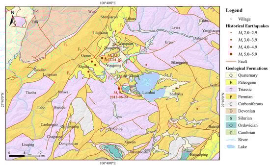
Figure 2.
The geological and tectonic map of the Ninglang area. (modified from the 1:200,000 regional geological map of G4705 Yongning [,,], F1 Wenquan Fault, F2 Yongning Fault, F3 Alaao Fault, F4 Rigulu-Yanwa Fault, F5 Anjiacun Fault; F6 Guangxishan Fault).
Since the Cenozoic, under the action of the modern tectonic stress field dominated by the near-horizontal NNW-oriented main compressive stress, two groups of NE- and NW-oriented fractures developed in the Ninglang area. Specifically, the NE-oriented and the NW-oriented fractures are dominated by left-slip motion and right-slip motion, respectively, and the two groups of fractures intersect each other to form a tessellated fracture pattern (Figure 2) [,,]. The seismic zone is dominated by the NW-oriented Wenquan Fault, the Yongning Fault, and the Alaao Fault, and the NE-oriented Rigulu-Yanwa Fault, the Guangxishan Fault, and the Anjacun Fault.
The Wenquan Fault, the Yongning Fault, and the Alaao Fault, have lengths of 16, 30, and 10 km, respectively, an overall strike of 290~335°, and a tendency to NE. They are mainly right-slip and orthotropic, and the latest activity is of the Late Pleistocene age. Among them, the Wenquan Fault and the Yongning Fault jointly control the east and west sides of the Yongning Basin, and they also affect the morphology of the Lugu Lake [,].
The Guangxishan Fault is a NE-oriented orthotropic fault with a strike of about 30°, a tendency to NW, and a dip of about 40°, and its generation period may be the late Variscan. The Anjacun Fault has a length of about 105 km, with a strike of about 40°, a tendency to NW, and a dip of about 40~50°. The former data from human exploration indicate that it is a high-angle reverse fault in nature, formed after the Jinning movement, and it has obvious signs of Early Paleozoic activity [,].
The Rigulu–Yanwa Fault consists of two faults, namely, the Gewayekou Fault and the Majiaping Fault, with a length of about 70 km. It starts in the Yanwa area to the southwest, passes through Rigulu, Lijiazu, and Luwabao to the northeast, and ends in the north of Wachang; meanwhile, it intersects with the NW Yongning Fault and other faults in Yongning and wadu. This fault is 45° in direction, with a NW dip in the main body and SE dip in the local area, with a dip angle of 40°~70°. It mainly recoils in the early stage and mainly left-slips since the Quaternary. It controls the Paleoproterozoic and Neoproterozoic basins such as Yanwa, Rigulu, and Lijiazu, and it is also a marginal fault of the Yongning Quaternary Basin [,].
3. Data and Methods
3.1. SAR Data and InSAR Processing
The traditional D-InSAR technique interferes differentially with two views of SAR images obtained at different times to obtain the surface deformation in the line of sight (LOS) direction of the two images. However, the accuracy of D-InSAR is often limited by topographic errors, atmospheric delays, and temporal decoherence. The SBAS-InSAR technique, developed from D-InSAR, pairs images according to a set spatio-temporal baseline threshold to form multiple interferometric pairs with short spatio-temporal baselines. As one of the time series InSAR techniques, SBAS-InSAR can eliminate the effects of spatio-temporal decoherence, atmospheric delayed phase, and topographic phase errors to obtain millimeter-scale deformation information of the study area. Currently, it is an indispensable tool for space-to-ground observations in seismotectonic studies [].
Suppose N + 1 SAR images covering the study area are acquired in a certain time period (t0,t1, … tN−1,tN) and one of them is selected as the master image for alignment. M differential interferograms can be obtained from a free combination of all differential interferometric pairs according to the set temporal and spatial baseline thresholds, where (Equation (1)):
After removing the effects of flat-earth and topographic phase, assuming that the jth differential interferogram (j∈(1, M)) is generated by acquiring the SAR image from the tB moment and the reference image at the tA moment (tB > tA), then the interference phase of the pixel at the azimuthal and distance coordinates (x,r) in the jth interferogram can be expressed as (Equation (2)):
where d(tB,x,r) and d(tA,x,r) are the cumulative deformations in the line of sight (LOS) direction at tB and tA, respectively, with respect to the initial moment t0. δφdef,j(x,r), δφtopo,j(x,r), δφatm,j(x,r), δφnoise,j(x,r), denote the deformation phase caused by displacement in the line of sight (LOS) direction, terrain phase error due to external DEM inaccuracy, and phase difference due to atmospheric delay and noise, respectively.
After estimating and removing the atmospheric phase, the elevation phase difference and the phase difference caused by noise, the phase φ is expressed as the product of the average phase velocity between any two acquisition times and the time. For M differential interferograms, the deformation time series can be expressed as (Equations (3)–(5)).
where A is the coefficient matrix of M × N. δφ is the unwrapped phase value vectors associated with the differential interferogram. Vlos and represent the LOS velocity vector and the LOS displacement at ti, respectively; A−1 represents the pseudo-inverse of matrix A which is evaluated using singular value decomposition (SVD) method [].
Sentinel-1A is a European radar imaging satellite launched in 2014. As the first Sentinel-1 satellite launched by the EU Copernicus program, it carries a C-band SAR with four imaging modes. In this study, the Single-look Complex (SLC) Level-1 product data of the Sentinel-1A satellite with interferometric wide-swath mode (IW) were selected to obtain coseismic deformation and seismic deformation time series by the InSAR technique. The spatial resolution of the data is 20 m × 5 m. The data were obtained from the European Space Agency (ESA) through the Alaska Satellite Facility Distributed Active Archive Centers (ASF DAAC). A total of 28 ascending orbit images and 30 descending orbit images from June 2021 to June 2022 in the Ninglang area were obtained, including the D-InSAR processed pre- and post-earthquake ascending and descending images of the Ninglang earthquake (Table 2). The size of the temporal and spatial baselines guarantees high coherence of the seismic zone data processing results. Then, the Shuttle Radar Topography Mission Digital Elevation Model (SRTM DEM) data (with a resolution of 30 m) released by the National Aeronautics and Space Administration (NASA) were used to simulate and remove the effect of the topographic phase. The satellite orbit information was obtained from the Precise Orbit Determination (POD) released by the ESA.
Table 2.
The parameter list of Sentinel 1A satellite images before and after the Ninglang Ms 5.5 earthquake in 2022.
The InSAR Scientific Computing Environment (ISCE) software developed by NASA Jet Propulsion Laboratory (NASA JPL) and Stanford University was employed for processing InSAR data []. Meanwhile, the two-pass D-InSAR method was used. The Goldenstein filtering method was exploited to obtain the filtered interferogram [], and 8 × 2 (Range × Azimuth) multilooking processing was performed in order to suppress the phase noise and improve the signal-to-noise ratio. Additionally, phase unwrapping was performed by using the Statistical-Cost Network-Flow Algorithm for Phase Unwrapping (SNAPHU) []. Finally, track errors were removed and re-deplaned by using the POD precision track data and SRTM DEM to obtain the coseismic deformation field (LOS) of the Ninglang Ms 5.5 earthquake after geocoding.
Before the SBAS-InSAR timing analysis, the SAR images were combined by using the TopStack module of ISCE to produce interferometric pairs. Then, a network-based enhanced spectral diversity method was applied to obtain high-precision alignment of the SLC images []. Interferograms were generated by a sequential interferogram network, and the interferograms were paired in time with their two closest neighbors. After the data preprocessing by using the ISCE performed, image registration, topographic phase estimation, and interferometric processing, MintPy was adopted to realize surface deformation time series inversion and mean rate estimation [], and Generic Atmospheric Correction Online Service for InSAR (GACOS) was applied to correct the InSAR atmospheric delay errors [], and the changes of displacement field before and after the Ninglang earthquake were obtained finally (Figure 3).
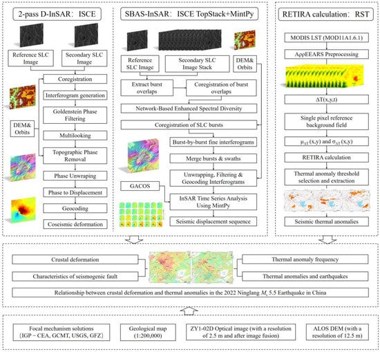
Figure 3.
The general research framework.
3.2. MODIS LST Data and RST Analysis
RST performs statistical analysis of multi-temporal data based on multi-year contemporaneous remote sensing satellite data in the same region, and it highlights the anomalies in the spatial domain relative to the temporal domain. After being proposed by Tramutoli et al., it was first used mainly with AVHRR-NOAA TIR data and thus called the RAT algorithm. Later, RST was extended to other remote sensing satellite data and has been applied to monitor natural and environmental disasters such as volcanic ash clouds [], volcanoes [], oil spills [], floods [], and forest fires []. In addition, RST has been applied to satellite thermal infrared monitoring in earthquake-prone areas by introducing the concept of signal-to-noise ratio (S/N) of seismic thermal anomalies. Specifically, the thermal anomalies caused by earthquakes are regarded as a signal (S), those caused by other factors are regarded as noise (N), and the S/N is exploited to express the intensity of thermal anomalies []. The thermal anomaly extraction threshold is selected to discriminate the thermal anomaly by calculating a specific indicator index (Robust Estimator of Thermal Infrared Anomalies, RETIRA) (Equations (6) and (7)).
where ∆T(x, y, t) is the difference relative to the regional thermal anomaly mean, μ∆T(x,y) is the multi-year mean of ∆T(x, y, t) in the same region over the same period, and σ∆T(x,y) is the standard deviation corresponding to the mean. The method constructs a robust background field of the signal, uses the Gaussian-like distribution characteristics of remote sensing data to calculate the deviation degree relative to the background field, i.e., to calculate the deviation degree of each image element in space relative to the background field, and uses ∆T(x, y, t) instead of T(x, y, t) to eliminate the influence of topography, meteorology, and other factors.
MODIS integrates 490 detectors and channels designed for 36 spectral bands with a spectral range from 0.4 to 14.5 μm, covering the visible to thermal infrared bands. It is carried on the polar-orbiting sun-synchronous satellites Terra and Aqua and the morning and afternoon stars. Thus, MODIS can obtain global observations (including daytime visible images and day/night infrared images) every one or two days. LST is an important indicator of the energy balance at the Earth’s surface, and it is a key factor in the physical processes at regional and global scales [].
In this paper, the MODIS LST (MOD11A1.6.1) at a resolution of 1 km from October to January 2013 to 2022 from the Terra satellite was selected to calculate the RETIRA index (Figure 3). Meanwhile, the nighttime observations were used to exclude surface temperature variations unrelated to seismic activities because solar radiation and topographic shadows can strongly interfere with the ground temperature information during the daytime. The data were obtained from Application for Extracting and Exploring Analysis Ready Samples (AρρEEARS) [], and the MODIS LST product was preprocessed with cropping and projection conversions. The MODIS LST used the MODIS cloud mask product, which contains only cloud-free pixels. The background field was constructed from 10 years of monthly MODIS LST data. Due to the formation of null areas caused by cloud pixel interference in the MODIS LST data, cloud coverage areas are too large, and the data may fail to reflect the regional mean. Thus, images with cloud pixel coverage greater than 80% were discarded in this study []. Additionally, spatial anomalies with a difference from the mean value greater than k (k ≥ 2) times the standard deviation were excluded []. Finally, the mean μ∆T and standard deviation σ∆T of the LST for each month in the seismic region was calculated, and the RETIRA indices of the screened images before and after the earthquake in Ninglang were generated (from June 2021 to June 2022).
4. Results
4.1. Coseismic Deformation
The ascending and descending interferograms and LOS-oriented deformation of the Ninglang earthquake on 2 January 2022 were obtained by using D-InSAR (Figure 4a–d). Due to the different satellite heading angles and incidence angles, different orbital coseismic deformation fields differ in position and magnitude but exhibit similar shapes. Meanwhile, the interference fringes have good coherence, and the overall shape is elliptical. Furthermore, the coseismic feature is more obvious and is located in the west of the epicenter. The orientation of the long axis of the coseismic deformation field of the ascending orbit is NW, and that of the descending orbit is nearly SN. The central part of the interfering streak is denser. Additionally, the coseismic deformation field is divided into northeast and southwest sides. The maximum settling deformation value and the maximum rising deformation value are −12.40 cm and +6.83 cm, respectively. The settling deformation is larger than the rising deformation, and the overall trend is subsidence. Moreover, in the interferogram of the descending orbit, the LOS deformation in the southwest side is opposite to the ascending orbit, while the northeast side is dominated by subsidence, and the right side of the epicenter shows a weak uplift deformation. The maximum subsidence deformation value and the maximum uplift deformation value are −6.06 cm and +5.69 cm, respectively.
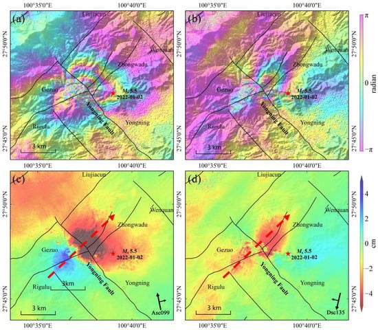
Figure 4.
The coseismic deformation field of 2022 Ninglang earthquake: (a) the ascending orbit interference fringe; (b) the descending orbit interference fringe; (c) the ascending orbit LOS deformation; (d) the descending orbit LOS deformation; The red star is the location of the epicenter given by the CENC. The red dashed arrow shows the location of the profile in Figure 5.
To understand the differences between the coseismic deformation fields, the profiles of the SW-NE orientation of the deformation fields are plotted at the same spatial location (Figure 5a,b). It can be seen that the tendency of the LOS-oriented coseismic deformation profiles in both the ascending and descending orbits is dominated by subsidence, which is consistent with the characteristic of the subsidence-dominated deformation caused by positive fault-type earthquakes. According to the relationship between the sink deformation zone and the uplift deformation zone in the coseismic deformation field, it can be initially assumed that the seismic rupture zone tends to the northeast. The northeast side is the upper wall of the normal fault, and the southwest side is the lower wall of the normal fault.
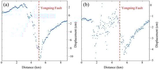
Figure 5.
(a) the coseismic deformation profile of the ascending orbit; (b) the coseismic deformation profile of the descending orbit.
4.2. Seismic Displacement Field
The SBAS-InSAR time series analysis of the interferometric pairs preprocessed by the ISCE TopStack was performed by using MintPy. The first view of the ascending and descending orbits image is taken as the baseline without deformation, where the ascending orbit is 1 June 2021, and the descending orbit is 3 June 2021. Then, the displacement field change process before and after the Ninglang earthquake and its deformation characteristics associated with the seismogenic rupture in the region at different stages were obtained.
To analyze the change law of the seismic displacement field with time, 20 points on both sides of the epicenter deformation zone in the pre- and post-earthquake displacement sequences of the ascending orbit InSAR (Figure 6), were selected to analyze their deformation time series (Figure 7a,b). A1–A10 are locate in the northeast subsidence area, and B1–B10 are locate in the southwest uplift area. After the earthquake (after 2 January 2022), the displacement field of the northeast side of the deformation field showed subsidence, and the southwest side showed an uplift. It can be seen from the obtained time series displacement field that the displacement had a clear phase with the earthquake occurrence: the region was basically in a state of small and slow deformation with small cumulative deformation from 1 June 2021 to 22 December 2021. The maximum accumulated deformation was about −3.53 cm, which is the pre-earthquake creeping displacement. From 22 December 2021 to 3 January 2022, across the epicenter moment, the deformation around the epicenter increased abruptly. The maximum value exceeded −7.27 cm, and the displacement changed rapidly and abruptly. After the earthquake on 3 January 2022, the deformation slowed down significantly, and the deformation continued to occur under the influence of small and medium-sized earthquakes on 5 January and April 2022. In the region, points A1–A10 showed a general downward trend, points B1–B10 showed a general upward trend, and all other points showed similar deformation trends.
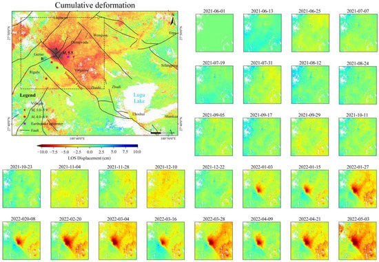
Figure 6.
The displacement time series before and after the earthquake of the ascending InSAR; A and B are the areas where the 20 selected deformation points (A1–A10, B1–B10) in Figure 7 are located.
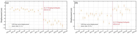
Figure 7.
(a) The deformation time series at point A1 to point A10; (b) The deformation time series at point B1 to point B10.
Similarly, the pre- and post-earthquake displacement sequences of the descending-orbit InSAR were analyzed (Figure 8, which excludes dates with large Root Mean Square (RMS)). From 1 June 2021 to 22 December 2021, the region was in a state of pre-earthquake creeping displacement in the period, which was consistent with the ascending track displacement sequence. After the earthquake on 2 January 2022, the deformation variables around the epicenter increased abruptly. Twenty points on both sides of the epicenter deformation zone were selected to analyze their deformation time series, all of which were dominated by subsidence and subsequent continuous deformation (Figure 9a,b). C1–C10 are located in the northeast subsidence area, and D1–D10 are located in the southwest subsidence area. The selected area is consistent with the ascending orbit. During the spanned time period, the obvious changes in the surface displacement field at different stages were consistent with the level of seismic activity in Ninglang, reflecting the accumulation, concentration, release, and adjustment process of strain energy.
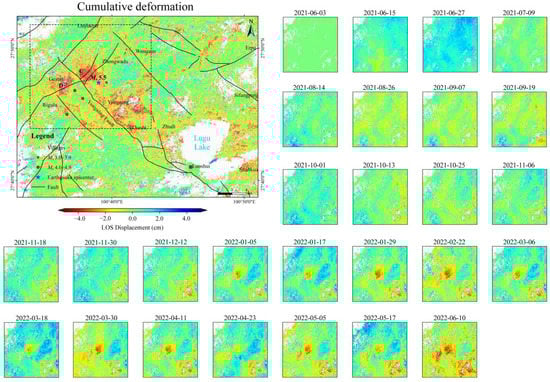
Figure 8.
The displacement time series before and after the earthquake of the descending InSAR. C and D are the areas where the 20 selected deformation points (C1–C10, D1–D10) in Figure 9 are located.
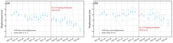
Figure 9.
(a) The deformation time series at point C1 to point C10; (b) The deformation time series at point D1 to point D10.
4.3. Seismic Thermal Anomalies
A total of 2431 images of MODIS LST data over a 10-year period (i.e., 2013–2022) were selected by pre-screening and filtering images with more than 80% cloud cover for the calculation of μ∆t(x, y) and σ∆t(x, y) of the RETIRA index. Each cloud-free image contains 1794 pixels, and the cloud-covered pixels in the image are identified as “Nodata”. The final RETIRA index was calculated for 255 images from June 2021 to June 2022, with 16 images in June, 12 in July, 13 in August, 21 in September, 26 in October, 27 in November, 28 in December, 28 in January, 25 in February, 26 in March, 17 in April, and 16 in May. A higher relative deviation threshold (RETIRA ≥ 3) was adopted, and a total of 23 anomalies were extracted before and after the earthquake.
By analyzing the distribution of the extracted thermal anomalies, it was found that the thermal anomalies appeared several times at the intersection of the Yongning fault and the ruptures in the region, especially in the Yongning, Zhashi, and northeastern Erpu and western Rigulu areas (Figure 10 and Figure 11). No thermal anomalies were extracted in June 2021 and June 2022.
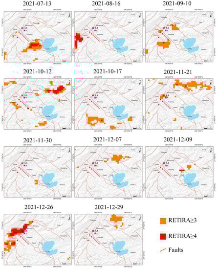
Figure 10.
The RETIRA thermal anomalies before the Ms 5.5 earthquake on 2 January 2022. The purple star and red circles are the epicenters in January and April, respectively.
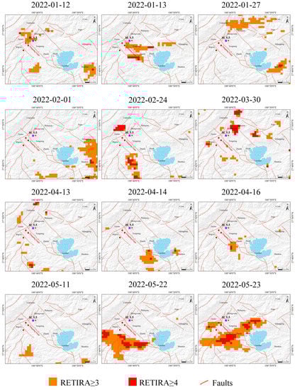
Figure 11.
The RETIRA thermal anomalies after the Ms 5.5 earthquake on 2 January 2022. The purple stars and red circles are the epicenters in January and April, respectively.
Before the Ms 5.5 earthquake on 2 January 2022, the thermal anomaly first appeared on 13 July in the southeastern section of the Yongning fault near Lugu Lake. A month later, on 16 August, a thermal anomaly appeared at the southwest end of the Rigulu-Yanwa Fault, and on 10 September, another thermal anomaly appeared near the Wenquan Fault and the Alaao Fault. On 12 October, a stronger thermal anomaly appeared in the Erpu area. Then, on 11 October and 12 October, thermal anomalies appeared in the southwestern and southern part of Yongning town, with RETIRA exceeding five in some areas. In addition, on 21 and 30 November, thermal anomalies appeared in the northern part of Yongning town, the Yongning fault zone, the Erpu area and the western side of Lugu Lake, respectively, and the epicenter area of the Yongning fault zone. From 7 December to 29 December, the thermal anomaly appeared again in the Erpu area, where the thermal anomaly appeared in October and November. During this period, several weak thermal anomalies appeared in the Yongning Fracture Zone, and a stronger thermal anomaly appeared on 26 December.
After the Ms 5.5 earthquake on 2 January 2022, thermal anomalies appeared again in the epicenter area, the Yongning Fault, and the northeast section of the Rigulu Fault on 12, 13, and 27 January. Thermal anomalies came to the east side of Lugu Lake on 27 January and 1 February. Subsequent thermal anomalies on 24 February, 30 March, and 13 April were more sporadically distributed near the rupture in the region. On 14 April and 16 April, the Yongning Fault on the west side of Lugu Lake showed thermal anomalies again, and in May the thermal anomalies migrated westward and northeastward, forming a larger-scale thermal anomaly with a higher RETIRA. The periodicity and reciprocity of the appearance of the thermal anomaly indicate strong rupture activity at this location.
5. Discussion
5.1. Characterization of Seismogenic Fault and Focal Mechanism Solutions
According to the characteristics of radar imaging geometry, the surface displacement in the LOS direction is a vector synthesis of the surface deformation in the north–south, east–west, and vertical directions projected in the LOS direction, respectively. For both uplifted and downgraded tracks, surface vertical deformation contributes to above 90% of the LOS-direction observations []. InSAR is most sensitive to the vertical deformation of the fault, and in terms of the coseismic deformation and the displacement field, the deformation is mainly dominated by subsidence before and after the earthquake. This is corroborated by the trend of the ascending and descending orbit deformation profile lines (Figure 5), showing the surface deformation caused by positive-fault type earthquakes. After superimposing the extent of the coseismic deformation zone on the remote sensing image with a resolution of 2.5 m of the resource satellite ZY-1 02D and Advanced Land Observing Satellite-1 DEM (ALOS DEM) with a resolution of 12.5 m, it can be seen that the deformation is mainly located in the northwest section of the Yongning Fault (Figure 12a,b). As the basin-controlling fault of the Yongning Basin, the Yongning Fault shows a straight linear extension with obvious topographic elevation differences on both sides, and steeply standing fault cliffs can be observed in the area from Yongning Town to Chenjiawan.
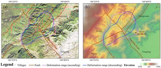
Figure 12.
(a) the ZY-1 02D remote sensing image superimposed deformation range; (b) the DEM superimposed deformation range; The red star is the location of the epicenter given by the CENC.
For a purely positive fault-type earthquake, the sinking deformation zone in the coseismic field should be located in the upper wall (northeast side in this region) of the normal fault, while the uplifting deformation zone should be located in the lower wall (southwest side) of the normal fault []. The uplift coseismic field acquired by InSAR is consistent with this property, i.e., the upper wall (northeast side) exhibits LOS to subsidence motion, the lower wall (southwest side) exhibits LOS to uplift motion, and the deformation volume of the upper wall is larger than that of the lower wall. However, the characteristics of the deformation field obtained by InSAR are not fully consistent with those of positive fault earthquakes; meanwhile, the lower wall (southwest side) shows LOS directional subsidence motion, so it is assumed that the Ninglang earthquake is dominated by positive fault and right-slip motion. During the relative motion of the upper wall descending on the orthotropic fault, the two walls will move in opposite directions of tension, causing uplift and subsidence changes in the southwest and northeast sides under different imaging modes of uplift and downgrade.
The solution of the source mechanism directly reflects the mechanical properties and motion of the earthquake rupture surface. Due to the different data used, the measured fault geometry and seismic source mechanism differ from one institution to another (Table 1). Overall, the two nodal directions of the fault are 183°~206° and 300°~316°, with dip angles of 41°~71° and 58°~81°, and sliding angles of −50°~−9° and −165°~−119°, respectively. Comparing the characteristics of the seismogenic rupture revealed by the isoseismic deformation and seismic displacement field obtained in this study with the solution of the seismogenic mechanism, the strike of 293°~316° is basically consistent with that of the Yongning Fault. Meanwhile, the fault type reflected by the dip angle also matches the kinematic characteristics of the Yongning Fault walking slip cum orthostatic rupture. Therefore, the NW-trending Yongning Fault is considered the seismogenic fault of this earthquake.
5.2. Thermal Anomalies and Earthquakes
The 23 days of seismic thermal anomaly information obtained using RST from June 2021 to June 2022 were overlaid and analyzed to study the spatial distribution and frequency (i.e., cumulative thermal anomalies of the same pixel). During these 23 days, the total number of thermal anomalies for each image element in the region was counted, and the 2 January earthquake was used as the boundary to obtain the preseismic, posseismic, and total thermal anomaly frequency distributions separately (Figure 13a–c).
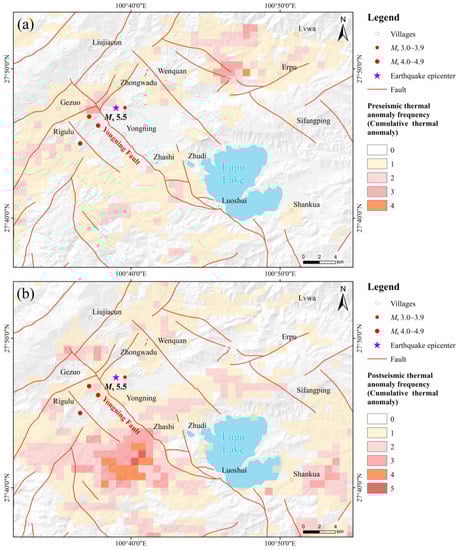
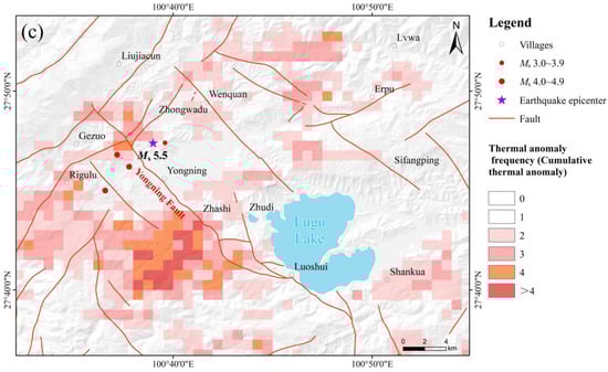
Figure 13.
(a) The frequency statistics of preseismic thermal anomalies; (b) The frequency statistics of postseismic thermal anomalies; (c) The frequency statistics of 23 thermal anomalies.
The preseismic thermal anomaly frequency ranges from 1 to 4 (Figure 13a) and is mainly distributed near the epicenter and its surrounding ruptures, especially in the northeastern part of Erpu. The postseismic thermal anomaly frequency ranges from 1 to 5 (Figure 13b) and thermal anomalies are mainly distributed in the southern part of the epicenter, the southwest side of the Yongning Fault, and some areas on the east side of Lugu Lake. The areas with the highest frequency of thermal anomalies before and after the earthquake are the western part of Erpu and the southwestern part of Zhashi, respectively, and there are certain common areas. After the Ms 5.5 earthquake on 2 January, four more earthquakes of magnitude 3~5 occurred in the region in April. The change in the concentration area of thermal anomalies may indicate that the post-earthquake thermal anomalies extracted for 12 days were associated with different earthquakes, superimposed on the pre-earthquake thermal anomalies in April, and that the earthquakes in January and April were independent of each other.
There is no research on the mechanism of seismic thermal anomalies in this region. Currently, many scholars have proposed theoretical theories to decipher the seismic thermal anomalies such as earth outgassing, stress heat generation, crustal rock cell conversion, latent heat release of radon decay, and multi-layer coupling effect by various methods, such as air electric field observation and rock loading radiation monitoring tests [,,,]. In particular, the first two are widely known, due to the intensification of pre-earthquake tectonic activities, the micro-fracture opening of rocks and ground surface in the region causes the underground enclosed gases such as H2, CO, CO2, CH4, Rn, etc., to escape from the ground along the fracture channels. Meanwhile, the warming effect of greenhouse gases will occur under the action of the atmospheric electric field. In addition, under the action of tectonic stresses, pre-earthquake deep subsurface fluids can be transported upward along fractures and fissures and decomposed into water and gases in the subsurface. Furthermore, the pre-earthquake crustal stress effect converts mechanical energy into thermal energy, which is transmitted to the surface through the pores in the rocks and the micro-rupture before the earthquake [,].
From the geological and tectonic background, two groups of NE- and NW-oriented fractures are developed in the area, forming a checkerboard fracture pattern. The spatial distribution of thermal anomalies is mainly in the NE-oriented Yongning Fault and the NW-oriented Rigulu–Yanwa Fault. The seismic fault system formed by the micro-rupture superimposed on the NE- and NW-oriented faults due to stress effects can provide a channel for the release of gas or thermal energy. The generation of thermal anomalies associated with the Ninglang earthquake may have the following stages: increasing stresses, forming micro-ruptures, leading to increased gas or thermal energy release [,,]. However, the stress field locally becomes high enough for the microfractures to close and the release of gas or heat energy to decrease until the earthquake occurs. At the time of the earthquake, there is a new increase in gas or heat energy release due to the creation of larger cracks in the fracture zone until the activity state in the zone gradually returns to normal [], such as the thermal anomaly in the epicenter for two consecutive days at different locations 10 days after the earthquake (12 and 13 January), and the two thermal anomalies in the area near the epicenter in May.
5.3. Relationship between Crustal Deformation and Thermal Anomalies
To further explore the relationship between the InSAR crustal deformation and seismic thermal anomalies of the Ninglang earthquake, the frequency distribution of thermal anomalies was superimposed on the cumulative crustal deformation obtained by SBAS-InSAR. Meanwhile, the time series of seismic thermal anomalies and deformation for 23 days are compared to further reveal the spatial and temporal correlation between the two different phenomena [].
In terms of time, the seismic displacement field obtained by InSAR indicates that the crustal deformation in the region undergoes a state of pre-earthquake creep—sudden change during the earthquake—continuous deformation, reflecting the activity information of active ruptures in the region. During the pre-earthquake creep, the thermal anomalies are mainly distributed at the intersection of ruptures around the epicenter, and the range of thermal anomalies gradually expands during the epicenter. After the sudden change during the earthquake, due to the rupture activity and the seismic activity in April, continuous deformation occurred in the region, and the thermal anomaly extended to other areas and increased in intensity.
Spatially, for the epicenter region, the frequency of thermal anomalies is higher in the northeast wall of the Yongning Fault than in the southwest wall, which corresponds to the larger deformation in the northeast wall than in the southwest wall obtained from the elevation track (Figure 14a,b); the frequency of thermal anomalies is positively correlated with crustal deformation variables. The relationship between crustal deformation and thermal anomalies in other regions is less obvious, but is mainly surrounded by areas with larger deformation variables.
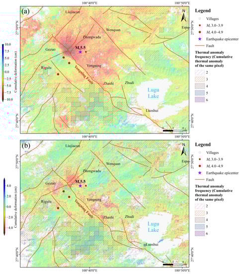
Figure 14.
(a) The thermal anomaly frequency superimposed on the ascending orbit deformation field; (b) The thermal anomaly frequency superimposed on the descending orbit deformation field.
The spatial and temporal correlation between crustal deformation and seismic thermal anomalies in the region, combined with the geological and tectonic background, confirms that the active rupture activity in the region generates deformation accompanied by changes in thermal radiation. The joint InSAR and RST reveal the spatial–temporal relationship between crustal deformation and seismic thermal anomalies in Ninglang, but further studies on the mechanism of seismic thermal anomalies in the region are needed.
5.4. Methodological Challenges
Since they were proposed, InSAR and RST techniques have been widely used to analyze earthquakes in several regions around the world. In this paper, InSAR and RST are exploited jointly for seismic monitoring and applied to the Ninglang earthquake of Ms 5.5 in the multi-earthquake region of northwest Yunnan, southwest China. However, the data and observations in this paper have certain limitations. Due to the operation mode of SAR satellite polar orbit and side-view imaging, when the fault orientation is nearly parallel to the satellite orbit direction, the slip displacement of the fault can hardly be observed by InSAR. Meanwhile, the crustal deformation obtained by InSAR is only the deformation of the Earth’s surface generating the LOS direction before and after the earthquake, so the surface motion characteristics of the fault obtained may be different from those of the deep part of the fault. In recent years, more and more scholars have combined multi-source data to invert the parameters of the seismogenic faults by using aftershock precision positioning and InSAR observations to further reveal the seismogenic characteristics [,].
For MODIS data, it is limited by the study area and the selected year or time, and it may be disturbed by clouds, especially in southwest China, thus leading to missing image elements. In addition, the mean values calculated in the spatial domain are not spatially representative. Thus, the use of related improved RST algorithms or reconstructed LST time series will improve the ability to detect seismic thermal infrared anomalies by using thermal infrared data. The fusion of multiple methods using multiple data is the future direction of seismic monitoring.
6. Conclusions
In this study, based on the combination of InSAR and RST analysis, a total of 58 views of Sentinel 1A imagery from June 2021 to June 2022 and 2431 views of MODIS LST daily nighttime observations from 2013 to 2022 were used to obtain the Ninglang earthquake coseismic deformation field, the InSAR displacement sequence of ascending and descending orbits before and after the earthquake, and the tectonic activity associated with surface thermal anomaly information. The conclusions are given below:
- (1).
- According to the crustal deformation, the seismic coseismic deformation mainly exhibits a subsidence-based deformation pattern, and the seismogenic faults are dominated by positive fault dip-slip motion. The seismic displacement field indicates that the cumulative deformation in the region is mainly caused by multiple small and medium-sized earthquakes in the epicenter, and the pre-seismic trend is stable and creeping displacement. Meanwhile, multiple earthquakes after the earthquake of Ms 5.5 on 2 January 2022 continued to generate deformation in the epicenter. Based on the solution of the source mechanism, it is considered that the NW-trending strike-slip-cum-positive rupture Yongning Fault is the seismogenic rupture of this earthquake.
- (2).
- From the thermal anomalies before and after the earthquake, the relative deviation threshold RETIRA ≥ 3 was selected, and 23 anomalies were extracted from June 2021 to June 2022. The seismic fault system composed of NE- and NW-oriented faults is an important factor in the formation of thermal anomalies, which are accompanied by changes in stress at different stages before and after the earthquake.
- (3).
- The active fracture activity in the zone produces deformation accompanied by changes in thermal radiation. Temporally, as the rupture activity intensifies, the thermal anomalies gradually expand outward from the rupture around the epicenter and become stronger as the deformation is generated. Spatially, the thermal anomalies are surrounded by the larger deformation zone, and the frequency of thermal anomalies in the area of obvious deformation in the epicenter is positively correlated with the deformation variation.
To sum up, microwave remote sensing is combined with thermal infrared remote sensing and applied to analyze the Ninglang earthquake in the southwest plateau region of China. The study results provide data support for the resolution of this earthquake and a reference for the application of multi-source remote sensing technology to earthquake monitoring.
Author Contributions
Conceptualization, Z.L. and Z.Z.; Data curation, Z.L. and J.C.; Formal analysis, X.Z.; Funding acquisition, Z.Z.; Investigation, W.C. and Y.Y.; Methodology, Z.L., J.C. and M.W.; Resources, Z.Z.; Software, Z.L., J.C., M.W. and J.L.; Validation, H.Y., W.C. and Y.Y.; Visualization, X.Z.; Writing—original draft, Z.L. and J.C.; Writing—review and editing, Z.Z., H.Y. and Q.C. All authors have read and agreed to the published version of the manuscript.
Funding
This study is supported by “National Natural Science Foundation of China” (Grant No. 41872251), “China-Myanmar Joint Laboratory for Ecological and Environmental Conservation” (K26202000920), “the Scientific Research Foundation of Yunnan Province Education Department” (Grant No. 2023Y0188), “the China Geological Survey Project” (Grant No. DD20221824), “Science and Technology Plan Project of Yunnan Province Science and Technology Department” (Grant No. 202101BA070001-145), “the List of Key Science and Technology Projects in the Transportation Industry of the Ministry of Transport in 2021” (Grant No. 2021-MS4-105).
Data Availability Statement
The Sentinel-1 data used in this study were downloaded from the European Space Agency (ESA) through the Alaska Satellite Facility Distributed Active Archive Centers (ASF DAAC, https://search.asf.alaska.edu/#/, accessed on 20 December 2022). The MODIS LST were obtained from Application for Extracting and Exploring Analysis Ready Samples developed by NASA’s LP DAAC (AρρEEARS, https://appeears.earthdatacloud.nasa.gov/, accessed on 20 December 2022). High resolution orthophoto was from Yunnan Remote Sensing Center. The ALOS DEM was downloaded from Japan Aerospace Exploration Agency (JAXA) through ASF DAAC.
Acknowledgments
The authors gratefully acknowledge the editor and anonymous reviewers for their constructive comments and suggestions on this paper. We thank ESA, NASA, JAXA, and Yunnan Remote Sensing Center for providing data for this paper. InSAR data processing in this paper was carried out using ISCE and MintPy software; some graphic elements were mapped by Generic Mapping Tools (GMT) [] and Matplotlib []. We would also like to express our gratitude to MJEditor (www.mjeditor.com) for providing English editing services during the preparation of this manuscript.
Conflicts of Interest
The authors declare no conflict of interest.
References
- Meng, Q.; Kang, C.; Shen, X.; Jing, F.; Qu, C. Seismic Infrared Remote Sensing, 2nd ed.; Seismological Press: Beijing, China, 2017; pp. 171–184. [Google Scholar]
- Zhang, P.; Deng, Q.; Zhang, G.; Ma, J.; Gan, W.; Min, W.; Mao, F.; Wang, Q. Strong Seismic Activity and Active Land Masses in Mainland China. Sci. China Ser. D-Earth Sci. 2003, 33, 12–20. (In Chinese) [Google Scholar] [CrossRef]
- Clark, M.R. Finding Active Faults Using Aerial Photographs. Earthq. Inf. Bull. (USGS) 1978, 10, 169–173. [Google Scholar]
- Tronin, A. Satellite Remote Sensing in Seismology. A Review. Remote Sens. 2009, 2, 124–150. [Google Scholar] [CrossRef]
- Mahmood, S.A.; Gloaguen, R. Appraisal of Active Tectonics in Hindu Kush: Insights from DEM Derived Geomorphic Indices and Drainage Analysis. Geosci. Front. 2012, 3, 407–428. [Google Scholar] [CrossRef]
- Gao, M.; Zeilinger, G.; Xu, X.; Wang, Q.; Hao, M. DEM and GIS Analysis of Geomorphic Indices for Evaluating Recent Uplift of the Northeastern Margin of the Tibetan Plateau, China. Geomorphology 2013, 190, 61–72. [Google Scholar] [CrossRef]
- Radaideh, O.M.A.; Mosar, J. Tectonics Controls on Fluvial Landscapes and Drainage Development in the Westernmost Part of Switzerland: Insights from DEM-Derived Geomorphic Indices. Tectonophysics 2019, 768, 228179. [Google Scholar] [CrossRef]
- Papanikolaou, I.; Dafnis, P.; Deligiannakis, G.; Hengesh, J.; Panagopoulos, A. Active Faults, Paleoseismological Trenching and Seismic Hazard Assessment in the Northern Mygdonia Basin, Northern Greece: The Assiros-Krithia Fault and the Drimos Fault Zone. Quat. Int. 2022. [Google Scholar] [CrossRef]
- Wright, T.; Parsons, B.; Fielding, E. Measurement of Interseismic Strain Accumulation across the North Anatolian Fault by Satellite Radar Interferometry. Geophys. Res. Lett. 2001, 28, 2117–2120. [Google Scholar] [CrossRef]
- Wright, T.J.; Parsons, B.; England, P.C.; Fielding, E.J. InSAR Observations of Low Slip Rates on the Major Faults of Western Tibet. Science 2004, 305, 236–239. [Google Scholar] [CrossRef] [PubMed]
- Taylor, M.; Peltzer, G. Current Slip Rates on Conjugate Strike-Slip Faults in Central Tibet Using Synthetic Aperture Radar Interferometry: Strike-slip sar rates, central tibet. J. Geophys. Res. 2006, 111, B12402. [Google Scholar] [CrossRef]
- Biggs, J.; Wright, T.; Lu, Z.; Parsons, B. Multi-Interferogram Method for Measuring Interseismic Deformation: Denali Fault, Alaska. Geophys. J. Int. 2007, 170, 1165–1179. [Google Scholar] [CrossRef]
- Wang, H.; Wright, T.J. Satellite Geodetic Imaging Reveals Internal Deformation of Western Tibet: Internal deformation of western tibet. Geophys. Res. Lett. 2012, 39, L07303. [Google Scholar] [CrossRef]
- Liu, C.; Ji, L.; Zhu, L.; Zhao, C. InSAR-Constrained Interseismic Deformation and Potential Seismogenic Asperities on the Altyn Tagh Fault at 91.5–95° E, Northern Tibetan Plateau. Remote Sens. 2018, 10, 943. [Google Scholar] [CrossRef]
- Liu, F.; Elliott, J.R.; Craig, T.J.; Hooper, A.; Wright, T.J. Improving the Resolving Power of InSAR for Earthquakes Using Time Series: A Case Study in Iran. Geophys. Res. Lett. 2021, 48, e2021GL093043. [Google Scholar] [CrossRef]
- Qiang, Z.; Xu, X.; Lin, C. Satellite Thermal Infrared Anomaly—Precursor of Imminent Earthquake. Chin. Sci. Bull. 1990, 35, 1324–1327. (In Chinese) [Google Scholar]
- Tramutoli, V.; Aliano, C.; Corrado, R.; Filizzola, C.; Genzano, N.; Lisi, M.; Martinelli, G.; Pergola, N. On the Possible Origin of Thermal Infrared Radiation (TIR) Anomalies in Earthquake-Prone Areas Observed Using Robust Satellite Techniques (RST). Chem. Geol. 2013, 339, 157–168. [Google Scholar] [CrossRef]
- Jing, F.; Shen, X.H.; Kang, C.L.; Xiong, P. Variations of Multi-Parameter Observations in Atmosphere Related to Earthquake. Nat. Hazards Earth Syst. Sci. 2013, 13, 27–33. [Google Scholar] [CrossRef]
- Bhardwaj, A.; Singh, S.; Sam, L.; Joshi, P.K.; Bhardwaj, A.; Martín-Torres, F.J.; Kumar, R. A Review on Remotely Sensed Land Surface Temperature Anomaly as an Earthquake Precursor. Int. J. Appl. Earth Obs. Geoinf. 2017, 63, 158–166. [Google Scholar] [CrossRef]
- Wu, L.; Qin, K.; Liu, S. Progress in Analysis to Remote Sensed Thermal Abnormity with Fault Activity and Seismogenic Process. Acta Geod. Et Cartogr. Sin. 2017, 46, 1470–1481. (In Chinese) [Google Scholar]
- Peleli, S.; Kouli, M.; Vallianatos, F. Satellite-Observed Thermal Anomalies and Deformation Patterns Associated to the 2021, Central Crete Seismic Sequence. Remote Sens. 2022, 14, 3413. [Google Scholar] [CrossRef]
- Tributsch, H. Do Aerosol Anomalies Precede Earthquakes? Nature 1978, 276, 606–608. [Google Scholar] [CrossRef]
- Tronin, A.A. Atmosphere-Lithosphere Coupling. Thermal Anomalies on the Earth Surface in Seismic Processes. In Seismo. Electromagnetics: Lithosphere-Atmosphere -Ionosphere Coupling; Hayakawa, M., Molchanov, O.A., Eds.; TERRAPUB: Tokyo, Japan, 2002; pp. 173–176. [Google Scholar]
- Okada, Y.; Mukai, S.; Singh, R.P. Changes in Atmospheric Aerosol Parameters after Gujarat Earthquake of 26 January 2001. Adv. Space Res. 2004, 33, 254–258. [Google Scholar] [CrossRef]
- Dey, S.; Sarkar, S.; Singh, R.P. Anomalous Changes in Column Water Vapor after Gujarat Earthquake. Adv. Space Res. 2004, 33, 274–278. [Google Scholar] [CrossRef]
- Massonnet, D.; Rossi, M.; Carmona, C.; Adragna, F.; Peltzer, G.; Feigl, K.; Rabaute, T. The Displacement Field of the Landers Earthquake Mapped by Radar Interferometry. Nature 1993, 364, 138–142. [Google Scholar] [CrossRef]
- Jiang, G.; Wen, Y.; Liu, Y.; Xu, X.; Fang, L.; Chen, G.; Gong, M.; Xu, C. Joint Analysis of the 2014 Kangding, Southwest China, Earthquake Sequence with Seismicity Relocation and InSAR Inversion: The 2014 kangding earthquake sequence. Geophys. Res. Lett. 2015, 42, 3273–3281. [Google Scholar] [CrossRef]
- Wang, H.; Liu-Zeng, J.; Ng, A.H.-M.; Ge, L.; Javed, F.; Long, F.; Aoudia, A.; Feng, J.; Shao, Z. Sentinel-1 Observations of the 2016 Menyuan Earthquake: A Buried Reverse Event Linked to the Left-Lateral Haiyuan Fault. Int. J. Appl. Earth Obs. Geoinf. 2017, 61, 14–21. [Google Scholar] [CrossRef]
- Zhao, D.; Qu, C.; Shan, X.; Bürgmann, R.; Gong, W.; Zhang, G. Spatiotemporal Evolution of Postseismic Deformation Following the 2001 Mw7.8 Kokoxili, China, Earthquake from 7 Years of Insar Observations. Remote Sens. 2018, 10, 1988. [Google Scholar] [CrossRef]
- Hamling, I.J.; Upton, P. Observations of Aseismic Slip Driven by Fluid Pressure Following the 2016 Kaikōura, New Zealand, Earthquake. Geophys. Res. Lett. 2018, 45, 11030–11039. [Google Scholar] [CrossRef]
- Zheng, A.; Yu, X.; Xu, W.; Chen, X.; Zhang, W. A Hybrid Source Mechanism of the 2017 Mw 6.5 Jiuzhaigou Earthquake Revealed by the Joint Inversion of Strong-Motion, Teleseismic and InSAR Data. Tectonophysics 2020, 789, 228538. [Google Scholar] [CrossRef]
- Tong, X.; Xu, X.; Chen, S. Coseismic Slip Model of the 2021 Maduo Earthquake, China from Sentinel-1 InSAR Observation. Remote Sens. 2022, 14, 436. [Google Scholar] [CrossRef]
- He, Y.; Wang, T.; Fang, L.; Zhao, L. The 2020 Mw 6.0 Jiashi Earthquake: Coinvolvement of Thin-Skinned Thrusting and Basement Shortening in Shaping the Keping-Tage Fold-and-Thrust Belt in Southwestern Tian Shan. Seismol. Res. Lett. 2022, 93, 680–692. [Google Scholar] [CrossRef]
- Ji, L.; Zhu, L.; Liu, C.; Zhang, W.; Qiu, J.; Xu, X. Review on InSAR-Derived Coseismic Deformation and the Determination of Earthquake Source Parameters. J. Earth Sci. Environ. 2021, 43, 604–620. [Google Scholar] [CrossRef]
- Berardino, P.; Fornaro, G.; Lanari, R.; Sansosti, E. A New Algorithm for Surface Deformation Monitoring Based on Small Baseline Differential SAR Interferograms. IEEE Trans. Geosci. Remote Sens. 2002, 40, 2375–2383. [Google Scholar] [CrossRef]
- Ferretti, A.; Prati, C.; Rocca, F. Permanent Scatterers in SAR Interferometry. IEEE Trans. Geosci. Remote Sens. 2001, 39, 8–20. [Google Scholar] [CrossRef]
- Ding, X.; Chen, H.; Zhang, W. SAR Monitoring of Nowaday Deformation in the Eastern Segment of the Altyn Tagh Fault. Earth Sci. Front. 2008, 15, 370–375. (In Chinese) [Google Scholar]
- Elliott, J.R.; Biggs, J.; Parsons, B.; Wright, T.J. InSAR Slip Rate Determination on the Altyn Tagh Fault, Northern Tibet, in the Presence of Topographically Correlated Atmospheric Delays: Altyn tagh fault slip rate. Geophys. Res. Lett. 2008, 35, L12309. [Google Scholar] [CrossRef]
- Daout, S.; Doin, M.-P.; Peltzer, G.; Lasserre, C.; Socquet, A.; Volat, M.; Sudhaus, H. Strain Partitioning and Present-Day Fault Kinematics in NW Tibet From Envisat SAR Interferometry. J. Geophys. Res. Solid Earth 2018, 123, 2462–2483. [Google Scholar] [CrossRef]
- Cavalié, O.; Lasserre, C.; Doin, M.-P.; Peltzer, G.; Sun, J.; Xu, X.; Shen, Z.-K. Measurement of Interseismic Strain across the Haiyuan Fault (Gansu, China), by InSAR. Earth Planet. Sci. Lett. 2008, 275, 246–257. [Google Scholar] [CrossRef]
- Xu, X.; Qu, C.; Shan, X.; Ma, C.; Zhang, G.; Meng, X. An Experimental Study of Monitoring Fault Crustal Deformation Using PS-InSAR Technology. Adv. Earth Sci. 2012, 27, 452–459. (In Chinese) [Google Scholar]
- Huang, Z.; Zhou, Y.; Qiao, X.; Zhang, P.; Cheng, X. Kinematics of the ∼1000 Km Haiyuan Fault System in Northeastern Tibet from High-Resolution Sentinel-1 InSAR Velocities: Fault Architecture, Slip Rates, and Partitioning. Earth Planet. Sci. Lett. 2022, 583, 117450. [Google Scholar] [CrossRef]
- Wang, H.; Wright, T.J.; Biggs, J. Interseismic Slip Rate of the Northwestern Xianshuihe Fault from InSAR Data: Interseismic slip rate of xsh fault. Geophys. Res. Lett. 2009, 36, L03302. [Google Scholar] [CrossRef]
- Walters, R.J.; Holley, R.J.; Parsons, B.; Wright, T.J. Interseismic Strain Accumulation across the North Anatolian Fault from Envisat InSAR Measurements: Naf interseismic strain from insar. Geophys. Res. Lett. 2011, 38, L05303. [Google Scholar] [CrossRef]
- Gornyy, V.; Sal’man, A.G.; Tronin, A.; Shilin, B.V. The Earth’s Outgoing IR Radiation as an Indicator of Seismic activity. Proc. Acad. Sci USSR 1988, 301, 67–69. [Google Scholar]
- Tramutoli, V. Robust AVHRR Techniques (RAT) for Environmental Monitoring: Theory and Applications. In Earth Surface Remote Sensing II.; Cecchi, G., Zilioli, E., Eds.; SPIE: Barcelona, Spain, 1998; pp. 101–113. [Google Scholar]
- Genzano, N.; Aliano, C.; Filizzola, C.; Pergola, N.; Tramutoli, V. A Robust Satellite Technique for Monitoring Seismically Active Areas: The Case of Bhuj–Gujarat Earthquake. Tectonophysics 2007, 431, 197–210. [Google Scholar] [CrossRef]
- Ouzounov, D.; Liu, D.; Kang, G.; Cervone, G.; Kafatos, M.; Taylor, P. Outgoing Long Wave Radiation Variability from IR Satellite Data Prior to Major Earthquakes. Tectonophysics 2007, 431, 211–220. [Google Scholar] [CrossRef]
- Genzano, N.; Aliano, C.; Corrado, R.; Filizzola, C.; Lisi, M.; Mazzeo, G.; Paciello, R.; Pergola, N.; Tramutoli, V. RST Analysis of MSG-SEVIRI TIR Radiances at the Time of the Abruzzo 6 April 2009 Earthquake. Nat. Hazards Earth Syst. Sci. 2009, 9, 2073–2084. [Google Scholar] [CrossRef]
- Song, D.; Zang, L.; Shan, X.; Yuan, Y.; Cui, J.; Shao, H.; Shen, C.; Shi, H. A Study on the Algorithm for Extracting Earthquake Thermal Infrared Anomalies Based on the Yearly Trend of LST. Seismol. Geol. 2016, 38, 680–695. (In Chinese) [Google Scholar] [CrossRef]
- Zhang, Y.; Meng, Q. A Statistical Analysis of TIR Anomalies Extracted by RSTs in Relation to an Earthquake in the Sichuan Area Using MODIS LST Data. Nat. Hazards Earth Syst. Sci. 2019, 19, 535–549. [Google Scholar] [CrossRef]
- Kouli, M.; Peleli, S.; Saltas, V.; Makris, J.; Vallianatos, F. Robust Satellite Techniques for Mapping Thermal Anomalies Possibly Related to Seismic Activity of March 2021, Thessaly Earthquakes. Bull. Geol. Soc. Greece 2021, 58, 105. [Google Scholar] [CrossRef]
- Institute of Geophysics, China Earthquake Administration A Briefing on Scientific and Technological Support for a Magnitude 5.5 Earthquake in Ninglang County, Lijiang City, Yunnan Province, On 2 January 2022. Available online: https://www.cea-igp.ac.cn/kydt/278803.html (accessed on 20 December 2022).
- Global CMT Search Results. Available online: https://www.globalcmt.org/cgi-bin/globalcmt-cgi-bin/CMT5/form?itype=ymd&yr=2022&mo=1&day=2&otype=ymd&oyr=2022&omo=1&oday=2&jyr=1976&jday=1&ojyr=1976&ojday=1&nday=1&lmw=5&umw=10&lms=0&ums=10&lmb=0&umb=10&llat=-90&ulat=90&llon=-180&ulon=180&lhd=0&uhd=1000<s=-9999&uts=9999&lpe1=0&upe1=90&lpe2=0&upe2=90&list=0 (accessed on 20 December 2022).
- M 5.4-99 Km E of Shangri-La, China. Available online: https://earthquake.usgs.gov/earthquakes/eventpage/us7000g8fk/origin/detail (accessed on 20 December 2022).
- GEOFON Event Gfz2022acjl: Yunnan, China. Available online: http://geofon.gfz-potsdam.de/eqinfo/event.php?id=gfz2022acjl (accessed on 20 December 2022).
- Deng, Q.; Zhang, P.; Ran, Y.; Yang, X.; Min, W.; Chu, Q. Basic characteristics of active tectonics of China. Sci. China Ser. D-Earth Sci. 2003, 46, 356–372. [Google Scholar] [CrossRef]
- Crippen, R.; Buckley, S.; Belz, E.; Gurrola, E.; Hensley, S.; Kobrick, M.; Lavalle, M.; Martin, J.; Neumann, M.; Nguyen, Q. NASADEM Global Elevation Model: Methods and Progress. Int. Arch. Photogramm. Remote Sens. Spat. Inf. Sci. 2016, 41, 125–128. [Google Scholar] [CrossRef]
- Wang, E.; Burchfiel, B.C.; Royden, L.H.; Chen, L.; Chen, J.; Li, W.; Chen, Z. Late Cenozoic Xianshuihe-Xiaojiang, Red River, and Dali Fault Systems of Southwestern Sichuan and Central Yunnan, China; Geological Society of America: Boulder, FL, USA, 1998; Volume 327, pp. 1–108. [Google Scholar]
- Wang, E.; Burchfiel, B.C. Interpretation of Cenozoic Tectonics in the Right-Lateral Accommodation Zone Between the Ailao Shan Shear Zone and the Eastern Himalayan Syntaxis. Int. Geol. Rev. 1997, 39, 191–219. [Google Scholar] [CrossRef]
- Xu, X.; Wen, X.; Zheng, R.; Ma, W.; Song, F.; Yu, G. The Latest Tectonic Change Patterns and Dynamic Sources of Active Blocks in the Sichuan-Yunnan Region. Sci. China Ser. D-Earth Sci. 2003, 33, 151–162. (In Chinese) [Google Scholar]
- Wu, Z.; Long, C.; Fan, T.; Zhou, C.; Feng, H.; Yang, Z.; Tong, Y. The Arc Rotational-Shear Active Tectonic System on the Southeastern Margin of Tibetan Plateau and Its Dynamic Characteristics and Mechanism. Geol. Bull. China 2015, 34, 1–31. [Google Scholar]
- Chang, Z.; Yang, S.; Zhou, Q.; Zhang, Y.; Xie, Y. Discussion of Seismogenic Structure of the June 24, 2012 Ninglang-Yanyuan Ms 5.7 Earthquake. Seismol. Geol. 2013, 35, 37–49. [Google Scholar]
- An, X.; Chang, Z.; Chen, Y.; Mao, X.; Zhuang, R. Quaternary Active Faults in Yunnan and “Distribution Map of Quaternary Active Faults in Yunnan”; Seismological Press: Beijing, China, 2018. [Google Scholar]
- Kan, R.; Zhang, S.; Yan, F.; Yu, L. Present Tectonic Stress Field and Its Relation to the Characteristics of Recent Tectonic Activity in Southwestern China. Chin. J. Sin. 1977, 20, 96–109. (In Chinese) [Google Scholar]
- Regional Geological Survey Report of G−47−5 1:200,000 in Yongning. Available online: http://www.ngac.org.cn/Data/archivesDetails?mdidnt=cgdoi.n0001%2Fx00068440 (accessed on 20 December 2022).
- Casu, F.; Manzo, M.; Lanari, R. A Quantitative Assessment of the SBAS Algorithm Performance for Surface Deformation Retrieval from DInSAR Data. Remote Sens. Environ. 2006, 102, 195–210. [Google Scholar] [CrossRef]
- Rosen, P.A.; Gurrola, E.; Sacco, G.F.; Zebker, H. The InSAR Scientific Computing Environment. In Proceedings of the EUSAR 2012, 9th European Conference on Synthetic Aperture Radar, Nuremberg, Germany, 23 April 2012; pp. 730–733. [Google Scholar]
- Goldstein, R.M.; Werner, C.L. Radar Interferogram Filtering for Geophysical Applications. Geophys. Res. Lett. 1998, 25, 4035–4038. [Google Scholar] [CrossRef]
- Chen, C.W.; Zebker, H.A. Phase Unwrapping for Large SAR Interferograms: Statistical Segmentation and Generalized Network Models. IEEE Trans. Geosci. Remote Sens. 2002, 40, 1709–1719. [Google Scholar] [CrossRef]
- Fattahi, H.; Agram, P.; Simons, M. A Network-Based Enhanced Spectral Diversity Approach for TOPS Time-Series Analysis. IEEE Trans. Geosci. Remote Sens. 2017, 55, 777–786. [Google Scholar] [CrossRef]
- Zhang, Y.; Fattahi, H.; Amelung, F. Small Baseline InSAR Time Series Analysis: Unwrapping Error Correction and Noise Reduction. Comput. Geosci. 2019, 133, 104331. [Google Scholar]
- Yu, C.; Li, Z.; Penna, N.T.; Crippa, P. Generic Atmospheric Correction Model for Interferometric Synthetic Aperture Radar Observations. J. Geophys. Res. Solid Earth 2018, 123, 9202–9222. [Google Scholar] [CrossRef]
- Pergola, N.; Tramutoli, V.; Marchese, F.; Scaffidi, I.; Lacava, T. Improving Volcanic Ash Cloud Detection by a Robust Satellite Technique. Remote Sens. Environ. 2004, 90, 1–22. [Google Scholar] [CrossRef]
- Pergola, N.; D’Angelo, G.; Lisi, M.; Marchese, F.; Mazzeo, G.; Tramutoli, V. Time Domain Analysis of Robust Satellite Techniques (RST) for near Real-Time Monitoring of Active Volcanoes and Thermal Precursor Identification. Phys. Chem. Earth Parts A/B/C 2009, 34, 380–385. [Google Scholar] [CrossRef]
- Casciello, D.; Lacava, T.; Pergola, N.; Tramutoli, V. Robust Satellite Techniques for oil spill detection and monitoring using AVHRR thermal infrared bands. Int. J. Remote Sens. 2011, 32, 4107–4129. [Google Scholar] [CrossRef]
- Lacava, T.; Filizzola, C.; Pergola, N.; Sannazzaro, F.; Tramutoli, V. Improving Flood Monitoring by the Robust AVHRR Technique (RAT) Approach: The Case of the April 2000 Hungary Flood. Int. J. Remote Sens. 2010, 31, 2043–2062. [Google Scholar] [CrossRef]
- Cuomo, V.; Lasaponara, R.; Tramutoli, V. Evaluation of a New Satellite-Based Method for Forest Fire Detection. Int. J. Remote Sens. 2001, 22, 1799–1826. [Google Scholar] [CrossRef]
- Pergola, N.; Aliano, C.; Coviello, I.; Filizzola, C.; Genzano, N.; Lacava, T.; Lisi, M.; Mazzeo, G.; Tramutoli, V. Using RST Approach and EOS-MODIS Radiances for Monitoring Seismically Active Regions: A Study on the 6 April 2009 Abruzzo Earthquake. Nat. Hazards Earth Syst. Sci. 2010, 10, 239–249. [Google Scholar] [CrossRef]
- Chao, J.; Zhao, Z.; Lai, Z.; Xu, S.; Liu, J.; Li, Z.; Zhang, X.; Chen, Q.; Yang, H.; Zhao, X. Detecting Geothermal Anomalies Using Landsat 8 Thermal Infrared Remote Sensing Data in the Ruili Basin, Southwest China. Environ. Sci. Pollut. Res. 2022. [Google Scholar] [CrossRef]
- AppEEARS Team Application for Extracting and Exploring Analysis Ready Samples (AppEEARS). Available online: https://lpdaac.usgs.gov/tools/appeears/ (accessed on 20 December 2022).
- Aliano, C.; Corrado, R.; Filizzola, C.; Genzano, N.; Pergola, N.; Tramutoli, V. Robust TIR Satellite Techniques for Monitoring Earthquake Active Regions: Limits, Main Achievements and Perspectives. Ann. Geophys. 2008, 51, 303–318. [Google Scholar] [CrossRef]
- Qu, C.; Shan, X.; Zhang, G.; Xu, X.; Song, X.; Zhang, G.; Liu, Y. The Research Progress in Measurement of Fault Activity by Time Series Insar and Discussion of Related Issues. Seismol. Geol. 2014, 36, 731–748. (In Chinese) [Google Scholar]
- He, P.; Wen, Y.; Ding, K.; Xu, C. Normal Faulting in the 2020 Mw 6.2 Yutian Event: Implications for Ongoing E–W Thinning in Northern Tibet. Remote Sens. 2020, 12, 3012. [Google Scholar] [CrossRef]
- Qiang, Z.; Kong, L.; Guo, M.; Wang, Y.; Zheng, L.; Lin, C.; Zhao, Y. An Experimental Study on Temperature Increasing Mechanism of Satellitic Thermo-Infrared. Acta Seismol. Sin. 1997, 19, 197–201. (In Chinese) [Google Scholar] [CrossRef]
- Deng, M.; Geng, N.; Cui, C.; Zhi, Y.; Fan, Z.; Ji, Q. The Study on the Variation of Thermal State of Rocks Caused by the Variation of Stress State of Rocks. Earthq. Res. China 1997, 13, 179–185. (In Chinese) [Google Scholar]
- Filizzola, C.; Corrado, A.; Genzano, N.; Lisi, M.; Pergola, N.; Colonna, R.; Tramutoli, V. RST Analysis of Anomalous TIR Sequences in Relation with Earthquakes Occurred in Turkey in the Period 2004–2015. Remote Sens. 2022, 14, 381. [Google Scholar] [CrossRef]
- Wessel, P.; Smith, W.H.F.; Scharroo, R.; Luis, J.; Wobbe, F. Generic Mapping Tools: Improved Version Released. Eos Trans. AGU 2013, 94, 409–410. [Google Scholar] [CrossRef]
- Hunter, J.D. Matplotlib: A 2D Graphics Environment. Comput. Sci. Eng. 2007, 9, 90–95. [Google Scholar] [CrossRef]
Disclaimer/Publisher’s Note: The statements, opinions and data contained in all publications are solely those of the individual author(s) and contributor(s) and not of MDPI and/or the editor(s). MDPI and/or the editor(s) disclaim responsibility for any injury to people or property resulting from any ideas, methods, instructions or products referred to in the content. |
© 2023 by the authors. Licensee MDPI, Basel, Switzerland. This article is an open access article distributed under the terms and conditions of the Creative Commons Attribution (CC BY) license (https://creativecommons.org/licenses/by/4.0/).