Toward Real Hyperspectral Image Stripe Removal via Direction Constraint Hierarchical Feature Cascade Networks

Abstract

In hyperspectral imaging (HSI), stripe noise is one of the most common noise types that adversely affects its application. Convolutional neural networks (CNNs) have contributed to state-of-the-art performance in HSI destriping given their powerful feature extraction and learning capabilities. However, it is difficult to obtain paired training samples for real data. Most CNN destriping methods construct a paired training dataset with simulated stripe noise for network training. However, when the stripe noise of real data is complex, destriping performance of the model is constrained. To solve this problem, this study proposes a real HSI stripe removal method using a toward real HSI stripe removal via direction constraint hierarchical feature cascade network (TRS-DCHC). TRS-DCHC uses the stripe noise extract subnetwork to extract stripe patterns from real stripe-containing HSI data and incorporates clean images to form paired training samples. The destriping subnetwork advantageously utilizes a wavelet transform to explicitly decompose stripe and stripe-free components. It also adopts multi-scale feature dense connections and feature fusion to enrich feature information and deeply mine the discriminate features of stripe and stripe-free components. Our experiments on both simulated and real data of various loads showed that TRS-DCHC features better performance in both simulated and real data compared with state-of-the-art method.

1. Introduction

With the continuous expansion of remote sensing image applications, the demand for hyperspectral imaging (HSI) applications is also increasing, especially in the domains of land cover classification, specific target detection and recognition, environmental monitoring, and precision agriculture [1,2,3,4]. HSI data have many bands, and are highly susceptible to interference during the imaging process by a series of degradation phenomena, such as thermal noise, impulse noise, stripe noise, and dead lines. These factors cause numerous adverse effects on his data processing, and the real spectral information is critically damaged, which constrains the application of HSI data. Therefore, the improvement of image quality in HSI data preprocessing is a key link in HSI data processing.

Of the many degradation factors, stripe noise is a common and special type of noise that usually has line characteristics. The main driver of stripe noise is the instability of a sensor and the inconsistent response of a sensor unit. For removal of the stripe noise, many methods have been proposed. Here, we divided the stripe removal methods into two groups: model-driven destriping method, and data-driven destriping method.

1.1. Model-Driven Destriping Method

Most of the traditional destriping methods belong to this category of methods. This kind of method usually designs an optimization model based on the generation mechanism of HSI stripes and prior knowledge of image processing for destriping [5]. Previously, for stripe removal, most traditional methods have used hand-crafted features to separate stripe components and stripe-free components. This allowed for the retrieval of a destriped image by analysis of the generation mechanism of the stripe based on prior knowledge [6,7,8,9]. They mainly used the frequency domain, non-local self-similarity, low rank, and sparse point of view to design filtering algorithms to perform the destriping operation [10,11,12,13]. For instance, Chen et al. [14] proposed a nonlocal tensor-ring approximation HSI denoising method based on tensor ring decomposition to explore the nonlocal self-similarity and global spectral correlation. Wei et al. [15] introduced an intra-cluster-structured low-rank matrix analysis HSI denoising method with automatically assigned rank numbers. Liu et al. [16] applied a 3D wavelet transform and low-rank model coupled with a group-sparse prior for pushbroom satellite image stripe removal. Wang et al. [17] focused on HSI mixed noise removal and constructed a multidirectional low-rank model combined with spatial-spectral total variation.

The wavelet-based method is a commonly used destriping method for model-driven destriping methods. Usually, the background of HSI data in the spatial domain is complex, and it is difficult to separate stripe and stripe-free components. The domain transforms an image from the spatial to the frequency domain. In the frequency domain, different image components exhibit different frequency signals, which can be used for effective distinction between stripe and stripe-free components [18]. Rasti et al. [19] proposed a wavelet-based sparse reduced-rank regression method for hyperspectral image restoration. Chen et al. [20] applied principal component analysis (PCA) and wavelet transform to remove noise in low-energy PCA output channels. Despite the considerable number of destriping methods, these traditional model-driven approaches are to some extent affected by image priors, and are limited by a handcrafted feature when the real stripe-contained HSI are more complex. Thus, these approaches cannot provide good performance in complex situations, and it is difficult to select and optimize model parameters.

However, these approaches, which had carefully designed handcrafted feature extraction operators based on the essential characteristics of stripes, cannot be used to fully characterize stripe and stripe-free components. Moreover, when the stripe generation mechanism and the feature extraction operator do not fit well enough, the destriping method applicability is limited.

1.2. Data-Driven Destriping Method

In recent years, researchers have been increasingly focusing on the application of CNN-based methods for HSI quality improvement. The CNN-based methods show a powerful feature representation ability due to the addition of the learning ability to the model itself; massive training data also play a pivotal role. Generally, most current methods for HSI destriping are based on supervised learning for model training, which requires a paired training dataset consisting of noisy images and corresponding clean images. However, it is difficult to acquire paired data [21]. To overcome this problem, synthetic noise can be added to a clean image to create paired data. Then, the simulated stripe-clean training pairs can be used to train the destriping network. For example, Cao et al. [22] proposed a deep spatial-spectral reasoning network for better denoising and restoration that considers both local and global context information. Zhang et al. [23] introduced a CNN-based method combining a spatial-spectral gradient image structure information prior network for HSI hybrid noise removal. Likewise, Zhong et al. [24] added image gradient information to the network as an auxiliary information to improve the stripe removal performance. On the other hand, by estimating the noise intensity as the training data feed to the model, which can efficiently adapt the model performance for noise at different intensities. Maffei et al. [25] designed a single network with a noise level map as input, which can remove noise in an efficient and flexible way. Furthermore, Yuan et al. [26] estimated the noise intensity through a dedicated subnetwork, which can improve the denoising ability of the model. Wang et al. [27] performed self-supervision by extracting noise samples from real data through a noise estimator. Subsequently, they added them to the clean band images in the data to form a noise-clean paired dataset. This method is advantageous but limited for determining the noise estimator and may affect extraction of noise samples. Song et al. [21] introduced a cycleGAN unsupervised stripe removal network based on a combined wavelet to solve the problem of difficult accessibility to paired data. Dong et al. [28] applied 3D UNet to combine spatial-spectral representation learning for HSI denoising. Chang et al. [29] proposed a CNN model with a wavelet, which achieved satisfactory results in a variety of stripe-type simulation experiments.

As the distribution of stripe noise is spatially random, expanding the receptive field using multi-scale feature extraction to obtain global features is a commonly used strategy. Liu et al. [30] proposed a denoising network based on the 3D pyramid dilation convolution to extract multiscale features. Chang et al. [31] developed HSI-DeNet interspersed with a dilation convolution layer to expand the receptive field and obtain multiscale features. Moreover, attention mechanisms have been extensively applied in the domain of computer vision [32,33,34], thus contributing to the state-of-the-art HSI processing. The attention mechanism has been broadly applied for HSI classification, semantic segmentation, pan sharpening, object detection, and change detection [35,36,37,38,39]. In recent years, attention mechanisms have also been applied in the image quality improvement domain. Anwar et al. [40] designed a real image blind denoising network with feature attention for extracting the dependency of inner channels. Shi et al. [41] applied 3D attention to deep aggregating the spatial-spectral feature for more efficient denoising.

The CNN-based method for HSI destriping has been extensively studied, yielding very promising methods and results. At present, most destriping methods are based on supervised learning, and training samples are generated by adding simulated stripes to clean samples. However, there is inconsistency between simulated stripes and real stripes that affects the model performance. This improves model performance in simulation experiments, but the real data performance remains instable. Notably, a large amount of real data has not yet been fully mined and utilized. The methods that consider real noise data used a threshold-based statistical approach to the extraction and estimation of realistic noise samples [27]. This kind of realistic noise sample extraction strategy is difficult to optimize, the parameters are complex, and it is more difficult to handle stripe pattern removal in complex situations. There have been fewer attempts to use the prior knowledge of the frequency domain to enhance the destriping performance of the model in a targeted manner.

1.3. Contributes

In response to the aforementioned challenges, this study proposes a solution based on full use of a large volume of real degraded data. Stripe samples for network training were obtained from real data samples, and from simulated stripe samples; they were then combined in synergy for training the samples. Theoretically, this solution enables the network to bridge the domain difference and break through the barriers between the simulated and the real stripe samples; moreover, it allows the model to exhibit better destriping performance on real data.

Thus, a real hyperspectral image stripe removal via a direction constraint hierarchical feature cascade network (TRS-DCHC) is proposed. The main innovations of TRS-DCHC can be summarized as follows:

• The training stripe samples for TRS-DCHC are both realistic and simulated data. On one hand, the model can process stripes with unknown distribution and structure. On the other hand, there is no need to thoroughly design the complicated stripe generation method; moreover, a blind destriping dataset can be obtained.
• In the stripe sample extraction and generation part, we mainly focus on spatial context information by adopting the strategy of extrapolating from local to global, and by proposing a constraint on the direction extraction strategy of points and lines, and lines and surfaces that extracts stripe samples from a global perspective.
• In the stripe removal part, we propose a multi-scale dense hierarchical feature cascading wavelet network through multi-scale feature extraction and multilevel feature fusion to obtain abundant information flow for the stripe component. In particular, we use the discrete wavelet transform (DWT) to explicitly decompose the input data into different frequency information as network input. This strategy combines the prior knowledge of an image with deep learning, which is more suitable for stripe removal. Moreover, it can alleviate the challenge of training, reduce information loss, and maintain spectrum consistency.

The remaining part of the manuscript is structured as follows. A systematic review of the HSI data stripe removal methods is described in Section 2. Details of the proposed destriping network are presented in Section 3. The experimental results and discussion are provided in Section 4. The main findings and the conclusions are summarized in Section 5.

2. Materials and Methods

In this section, we introduce the HSI degradation formula and describe the proposed TRS-DCHC in detail. As illustrated in Figure 1, the unified HSI destriping algorithm can be divided into two modules: a direction-constrained stripe adaptive extraction subnetwork, and a wavelet-based hierarchical feature cascaded destriping subnetwork.

2.1. HSI Degradation Formula

HSI spaceborne systems are susceptible to interference caused by environment-related and instrumental factors during the imaging process, which produce stripe noise. Generally, the HSI stripe noise model can be expressed as

$$Y=C+S$$

(1)

where Y denotes an observed three-dimensional (3D) HSI cube of size W × H × B, and W, H, and B denote the width, height, and band number of the HSI cube, respectively. C is a stripe-free component and S denotes a stripe component. The goal of destriping is to obtain the restored stripe-free component. Moreover, all the stripes should be empirically considered as additive components.

The models trained by simulated stripe-clean pairs can achieve satisfactory results in simulation experiments; however, the stripes are more complex than the simulated stripes in real situations, and when the real situation is inconsistent with the simulated stripe, the trained model cannot be well migrated to real situations. This limits their application in real situations.

2.2. Direction Constrained Stripe Adaptive Unsupervised Extraction Subnetwork

To improve the destriping ability of the model, we take full advantage of large volumes of real noisy data. In particular, we extract stripe samples from real data and change the single stripe-clean training paired construction mode to generate a specific distribution of simulated stripe samples. The direction-constrained stripe adaptive extraction subnetwork adopts a local-to-global, point-to-line, and line-to-surface strategy, leading to unsupervised adaptive extraction of stripe patterns in real data; the structure of the extraction subnetwork as shown in Figure 2a.

The direction-constrained stripe adaptive extraction subnetwork consists of a convolution layer (Conv), ReLU layer, residual block (RB), and direction-constrained spatial context module (DCSC). The DCSC structure is shown in Figure 2b, and is composed of two modules: a spatial context aggregation residual block (SCARB), and a multi-direction awarded local to global module (MDL2G), as displayed in Figure 2c,d. We use structures such as image spatial recurrent neural network (IRNN) [42] to aggregate the spatial context information with two stages of recurrent translations in a local to global manner. To this end, we apply four fixed directions to accurately capture stripe patterns from real data.

We designed the MDL2G module using the aforementioned IRNN architecture. The MDL2G retrieves global context information by executing a four-direction-aware IRNN twice and the feature extraction process of the IRNN, as shown in Figure 3. In the first stage, the information in the four directions (up, left, down, right) of each position in the input feature map is recursively obtained through a 1 × 1 convolution. Then, the output feature map (denoted as F), which collects each position for contextual information in the horizontal and vertical directions, and the recurrent convolution operation is repeated for F in the second stage. After the convolution operation (embedded in the first two stages), the global context information of the feature map can be obtained to realize the extraction of global feature information from the local to the global context.

Moreover, to obtain and learn spatial context information more specifically, we also designed another branch. This step was required to further extract the discriminate stripe feature using the sigmoid function and to directly generate the attention map of the input feature map. The latter can be used as guidance information. Moreover, it can provide auxiliary information for more accurate extraction of stripe patterns.

As the data with real stripes do not contain corresponding ground truth data, they are unsupervised in the real stripe sample extraction process. Hence, the model cannot be trained by calculating the loss between the network output and ground truth as supervised learning. Rudin et al. [43] has demonstrated that the total variation (TV) of noise-contained images is larger than that of clean images. Owing to this, we used TV loss as the loss function of the extraction subnetwork during the training process. As the extraction subnetwork is aimed to generate stripe patterns from real stripe-contained data, which are more complex and random than simulated stripes, it does not concentrate on the consistency between the extracted stripe and the stripe on the real image. Therefore, it can be constrained by TV loss, which is calculated by

$$L_{\mathrm{TV}}={‖{\nabla }_{h}I‖}_2^2+{‖{\nabla }_{v}I‖}_2^2$$

(2)

where I denotes the image subtracted by the input image to the output one, and ${\nabla }_h$ and ${\nabla }_v$ are the horizontal direction gradient and vertical direction gradient, respectively.

2.3. Wavelet-Based Hierarchical Feature Cascaded Destriping Subnetwork

HSI data have a highly complex background and contain rich spectral information It is challenging to effectively distinguish stripe patterns and ground objects, thereby, hampering the HSI stripe removal. Features at different levels and frequency represent different types of information. Low-level features represent more specific features, whereas high-level features are more abstract. The fusion of features at different levels can enable the network to learn more discriminating features that distinguish the patterns (stripe or strip-free).

2.3.1. Wavelet Decomposition

It should be noted that the input data of the wavelet-based direction-constrained stripe adaptive extraction subnetwork are no longer the original image data, but wavelet sub-bands (coefficients) [44] after DWT. Image data can be explicitly decomposed from the spatial domain transform to the frequency domain into different frequency information through wavelet transformation. This removes the complexity in the calculation and information loss. Here, we utilize the Haar wavelet transform as the mapping method between the image data and frequency domain. Let I denote the input image data, the Haar wavelet transform which decomposes I into four sub-band images through four bandpass filters: approximation of image (LL), horizontal detail (LH), vertical detail (HL), and diagonal detail (HH) bands [45]. Given the orthogonality of the DWT filter, the image can be reconstructed by the inverse wavelet transform (IWT). As stripe patterns usually emerge with certain directional characteristics, they exhibit certain performance in fixed coefficients after DWT operation. As shown in Figure 4, stripe patterns show notable performance in vertical coefficients, but insignificant in the horizontal and diagonal coefficients. Owing to this, we combine DWT with CNN to provide prior information for the extraction subnetwork and to ultimately improve the efficiency of extracting stripe patterns.

2.3.2. Multi-Scale Hierarchical Feature Fusion

Multi-scale feature extraction and residual learning are widely used for the remote sensing image processing. In the wavelet-based hierarchical feature cascaded destriping subnetwork, we use dense connections to better retain detailed information to reduce the information loss in the feature extraction process. Further, MsRB applies inter-layer multi-scale feature aggregation to obtain multi-scale features to enhance the information extraction ability, which is beneficial for improving the destriping performance.

Specifically, we use a two-stage structure to extract and fusion multiscale features in MsRB. The input feature F passes through convolutional layers with kernel sizes of 3 × 3, 5 × 5, and 7 × 7, and retrieves features F_{3_1}, F_{5_1}, and F_{7_1}, respectively. Then, concentrate operation is performed on F_{3_1}, F_{5_1}, and F_{7_1}, and the concentrate result is passed through the convolutional layer with kernel sizes of 3 × 3, 5 × 5, and 7 × 7 to perform feature extraction again to obtain F_{3_2}, F_{5_2}, and F_{7_2}; this operation is performed iteratively. Through two multi-scale feature extracts and feature fusion, MsRB can learn the primary features of the input feature. A global skip connection is introduced to prevent gradient explosion and feature information loss. As the depth of the network increases, the extracted features become more abstract and more significant. Therefore, the fusion of features at different levels can provide richer feature information and mine more representative and discriminatory information.

The mean square error (MSE) is then introduced as the loss function for the destriping subnetwork, which is defined as

$$L_D=\frac{1}{2n}{\displaystyle \sum _{i=1}^n‖X_i-}{R_i‖}^2$$

(3)

where n denotes the number of batches, X denotes the clean image, and R is the destriped image.

3. Experimental Results and Discussion

To evaluate the effectiveness of the proposed method, we provide the details of the training data and verification data, while also providing training parameter settings, evaluation indicators, and ablation experiments. We conducted experiments on simulated and real stripe contained data with different loads and compared them with various representative methods.

3.1. Experimental Datasets and Parameter Setting

We selected 22 Chinese GaoFen-5 (GF-5) hyperspectral satellite images as the real stripe-containing dataset for stripe pattern extraction; the images measured 2008 × 2083. The GF-5 satellite is an advanced hyperspectral imager (AHSI) with visible and near-infrared (VNIR) and shortwave infrared (SWIR) sensors [46]. GeoFen-5 is a polar-orbiting satellite of the China High-Resolution Earth Observation System (CHEOS) belonging to the China National Space Administration; it was launched in 2018 [47]. The VNIR sensor has 150 bands, and the SWIR has 180 bands. Figure 5 shows a segment of the real data for the stripe extraction used in this study. Moreover, we selected the Washington DC Mall his dataset (WDC) as the training and simulation test data. For the real data experiment, we selected the GF-5 data, Chinese ZhuHai-1 hyperspectral satellite (ZhuHai-1) data, Earth Observing-1 (EO-1) image data, and HYDICE UrbhisHSI data as the test data in the real data experiment. The

Table 1. Characteristic of The Experimental Datasets.

	Dataset
	WDC	GF-5	ZhuHai-1	EO-1	Urban
Size	1208 × 307 × 191	2008 × 2083 × 150/2008 × 2083 × 180	512 × 512 × 32	200 × 200 × 210	307 × 307 × 210
Sensor	Hydice	AHSI	CMOS	Hyperion	Hydice

list the characteristic of the datasets mentioned above. At the data processing stage, foremost, we normalized the real stripe-containing data and the WDC data to (0, 1), and then cut the data into sub-cubes of size 64 × 64 × 10; the rotation and flip operation were performed for data augmentation. Shuffle is performed before entering the next epoch. The total loss of the TRS-DCHC can be defined as

$$L_{total}=\lambda L_{\mathrm{TV}}+L_D$$

(4)

The proposed method was implemented on a Python 3.6 environment with the Pytorch package and NVIDIA Tesla V100 GPU. For the training phase, the ADAM solver [48] was applied as the optimizer with β = (0.9, 0.999), and the learning rate was fixed at 0.0001. The epoch was set as 300 with batch size = 64, λ set as 0.01 empirical.

In addition, to evaluate the effectiveness of the proposed TRS-DCHC (The code is available in https://github.com/November666/TRS-DCHC (accessed on 12 December 2021)) method, we selected current state-of-the-art methods, that is, ASSTV [49], LRTV [50], NGMeet [51], LRMR [52], TDL [53], HSI-DeNet [31], and SGIDN [24], for comparison. For the accurate comparison, the evaluation indices, peak signal-to-noise ratio (PSNR), and structural similarity (SSIM) [54] indices were used for the simulated experimental destriped image quantitative assessment. For the real experiment, there was no reference, thereby constraining quantitative evaluation. To overcome this constraint, we used no-reference indices (an inverse coefficient of variation (ICV) [55] and the mean relative deviation (MRD) [56]) to quantitatively evaluate the effect of destriping. Furthermore, we performed land-cover mapping on the destriped image to verify the destriping performance.

3.2. Simulated Data Experimental Results and Analysis

In the simulated experiment, we designed a variety of stripe types to confirm the destriping performance of the TRS-DCHC method, and designed three simulated stripe patterns as follows:

Case 1 (Period Stripe): the stripe intensities obey a normal distribution with standard deviation σ = 25; in different bands, the intensities are the same.

Case 2 (Random stripe): the stripe intensities obey a normal distribution with random standard deviation σ ∈ [10, 49], and in different bands, the intensities are different.

Case 3 (Stripe noise and dead lines): added stripe noise and dead lines obey the normal distribution with random standard deviation σ = 20.

The evaluation results are shown in

Table 2. Quantitative Evaluation of Simulated Experiments.

	Case 1		Case 2		Case 3
	MPSNR	MSSIM	MPSNR	MSSIM	MPSNR	MSSIM
LRTV [50]	30.21	0.8206	29.26	0.7661	25.37	0.6427
LRMR [52]	27.27	0.7102	28.91	0.7850	26.54	0.6771
TDL [53]	27.51	0.7099	27.81	0.7364	26.16	0.6555
NGMeet [51]	28.06	0.7434	33.64	0.8565	33.76	0.8703
ASSTV [49]	29.36	0.7542	32.63	0.8423	33.61	0.8626
HSI-DeNet [31]	36.17	0.9128	34.69	0.8974	33.84	0.8741
SGIDN [24]	35.97	0.9036	35.85	0.9002	34.33	0.8846
DCHC	42.83	0.9786	36.07	0.9013	36.86	0.9025
TRS-DCHC-noW	42.21	0.9675	35.63	0.8942	36.07	0.8870
TRS-DCHC	43.04	0.9867	36.22	0.9170	36.91	0.9078

. We also show the destriping results without incorporated real data (denoted as DCHC) and incorporated real data but without wavelet (denoted as TRS-DCHC-noW). The best results are indicated in bold. The simulated destriping results are displayed in Figure 6, Figure 7 and Figure 8 with pseudo color images (bands: 57, 27, and 17). In Case 1, LRTV has a good processing effect (see Figure 6). Moreover, Figure 6e,f) shows that LRMR, TDL, and NGMeet are not very effective in processing periodic stripe noise, and there are still large areas of stripe residue. In particular, NGMeet also introduces the problem of spectral loss. The stripe removal ability of ASSTV was better than that of the previously mentioned methods. It exhibits some suppression impact on stripes, but the impact is limited. Figure 6g shows considerable stripe noise that has not been completely removed. Considering the CNN-based methods, HSI-DeNet and SGIDN have prominent processing effects on stripes, which can remove nearly all stripes, but the consistency of the spectral information of the destriped image is poor; especially for HSI-DeNet where there is loss of detail (see Figure 6h for details). TRS-DCHC stands out with promising advantages in stripe removal, as it can remove all stripes and can achieve satisfactory results in the recovery of the destriped image, which is basically the same as the original image.

The results of Case 2 are shown in Figure 7. As can be seen, LRTV can partially alleviate stripe noise, but it cannot completely suppress it. Moreover, a problem of large spectral changes emerges as shown in Figure 7c. Although LRMR has a small loss of spectral information, it cannot completely remove all stripe noise, as seen from Figure 7d. The destriped result of TDL, similar to LRTV, is displayed in Figure 7e. It suffers from the same problem of incomplete stripe removal and the loss of spectral information. NGMeet has a prominent effect on stripe removal by removing nearly all stripes, but it also destroys the original spectral information of ground features, as shown in Figure 7f. ASSTV removes a large area of stripe, and the spectral information is retained better; however, the stripe residues are not completely suppressed in some areas, as can be seen in Figure 7g. Figure 7h demonstrates that the HSI-DeNet has no prominent stripe residues, but the balance between stripe removal and image restoration is plagued. In particular, the processed image has a certain amount of blur and loss of detail. The destriping performance of SGIDN is good; however, there are a few areas where details are not completely restored (see Figure 7i). The TRS-DCHC can provide relatively satisfactory results in stripe removing and image recovery as the stripe is nearly completely removed, and the spectral information is close to the original image with minimal loss.

Figure 8 shows that for Case 3, the stripe noise mixed with dead lines hampers the stripe removal. LRTV, LRMR, and TDL do not perform well on the stripe-mixed dead lines. In particular, LRTV also triggers the loss of spectral information, as shown in Figure 8c–e. NGMeet has a strong inhibitory effect on stripe, but it shows nearly no efficiency in the treatment of the dead lines. Moreover, it cannot provide an obvious repair effect on the dead lines, as indicated by Figure 8f. Likewise, ASSTV has a significant inhibitory effect on stripes, but it does not eliminate the dead lines. At the same time, the spectral information is affected to some extent, as shown in Figure 8g. HSI-DeNet has a good suppression effect on stripe and the dead lines. Figure 8h demonstrates that most of the stripes can be removed, but a small part of the stripe remains. In terms of the dead lines, HSI-DeNet can also provide a better restoration effect; however, the overall spectral information of the restored image changed. SGIDN has a prominent effect on the processing of stripe noise. There is no large area of stripe residue, except for a small part of the stripe that has not been well processed. The dead lines can also be better repaired and the spectral of the repaired image can be obtained. A better retention is identified, as shown in Figure 8i. TRS-DCHC not only has the ability to remove stripes, but it can also repair dead lines with satisfactory results, as shown in Figure 8j.

From the index evaluate results, as reported in Table 2, the DCHC and TRS-DCHC -noW can also provide a better destriping performance. However, the overall index of TRS-DCHC was the best, the performance was relatively stable, the processing of various stripes was with facility, and the repair performance was also ideal. Both visual comparison and quantitative comparison proved the superiority and the efficiency of TRS-DCHC compared to previous approaches.

3.3. Real Data Experimental Results and Analysis

Examination of the destriping performance on real data is a more realistic way to evaluate the effectiveness of the method. To this end, we considered a real data experiment and selected seven scenes of the HSI data with different loads (GF-5, Zhuhai-1, Hyperion EO-1, and HYDICE Urban datasets) to confirm the effectiveness and competitiveness of the TRS-DCHC method. These real data contain various levels of complex stripes and hybrid noise, which represent complex state-of-the art challenges for HSI destriping methods. We selected an area of 10 × 10 to calculate MRD and ICV. The evaluation results are shown in

Table 3. Quantitative Evaluation Results for Real Data Experiments.

Images	Index	Methods
		LRTV	LRMR	TDL	NGMeet	ASSTV	HSI-DeNet	SGIDN	DCHC	TRS-DCHC-noW	TRS-DCHC
GF-5 Scene 1	MRD	1.763	1.787	2.490	3.731	1.706	3.309	1.605	3.830	3.508	3.599
	ICV	8.031	8.685	8.428	6.915	7.924	5.906	7.767	12.141	11.505	13.341
GF-5 Scene 2	MRD	0.778	0.555	3.218	3.838	1.002	1.101	1.506	0.539	0.630	0.522
	ICV	2.590	2.772	2.912	3.334	2.333	2.226	1.945	3.326	3.491	3.863
GF-5 Scene 3	MRD	4.368	2.904	2.929	2.523	2.196	5.129	7.428	4.020	3.334	3.623
	ICV	5.393	3.723	3.747	4.062	2.863	3.441	6.493	2.408	3.590	3.317
Zhuhai-1 Scene 1	MRD	1.804	2.176	1.961	1.539	1.382	1.415	2.697	2.052	1.126	0.960
	ICV	5.335	4.996	4.525	4.872	5.170	4.434	4.012	5.120	5.377	5.443
Zhuhai-1 Scene 2	MRD	2.813	1.680	1.308	1.672	1.539	0.820	4.384	1.374	1.283	1.134
	ICV	3.607	3.913	4.260	4.765	4.475	4.368	5.261	4.310	4.235	5.484
Hyperion EO-1	MRD	2.160	2.663	2.788	2.383	2.738	3.185	2.929	2.532	2.193	2.375
	ICV	2.507	1.854	2.102	2.044	1.978	2.606	1.953	2.672	2.598	2.714
HYDICE Urban	MRD	2.209	2.292	3.011	3.177	1.878	1.936	1.986	2.044	1.895	1.779
	ICV	0.785	0.779	0.8992	0.729	0.754	1.118	0.688	0.795	1.051	1.387

; similarly, we also report the quantitative evaluate results of DCHC and TRS-DCHC-noW. Therein, the best results for each scene are marked in bold, and the second-best results are marked in blue.

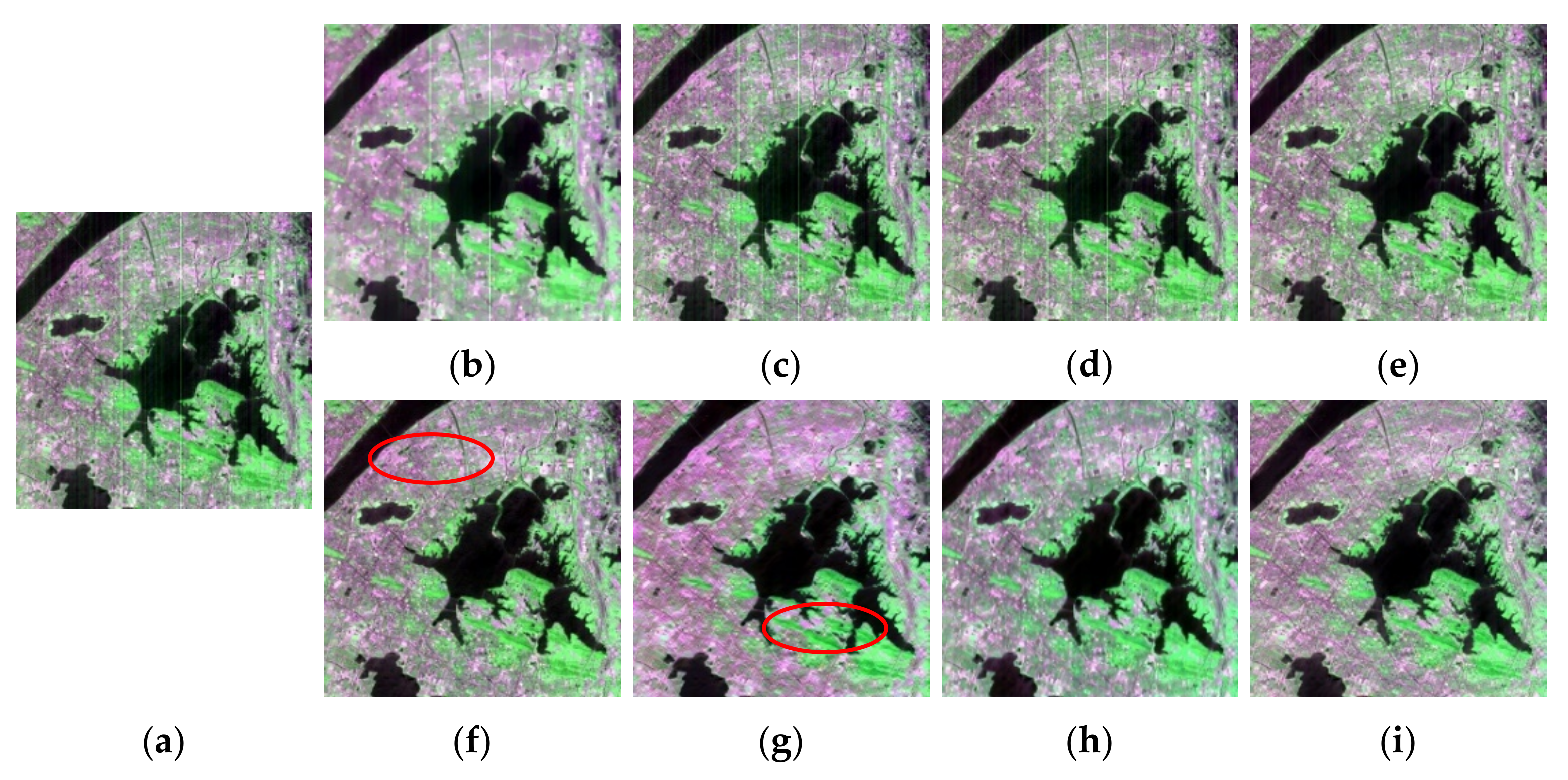
3.3.1. GF-5 HSI Dataset

We selected two scenes of GF-5 data for the real data experiment corrupted by mixed stripe and random noises. The destriped results are presented in Figure 9 and Figure 10. Some unobvious stripe residues or spectral loss areas are marked by the red eclipse.

For scene 1 with 512 × 512 × 180 size, the original image contained many stripes, and the noise level is strong. The experimental results show that although LRTV can suppress a portion of the stripe noise (see Figure 9b), the structure and texture of the stripe-free component of the image itself are destroyed. LRMR and TDL are not effective with stripe removal, as can be seen in Figure 9c,d. After the NGMeet processing, most of the stripe noise is removed over land, but the residuals of strip noise are evident over the water body. A small fraction of strips is not completely removed, and the spectral information of the destriped image also differs from that of the original image, as illustrated in Figure 9e. Further, Figure 9f shows that the ASSTV method has a good inhibitory effect on the stripe; the striped result has prominent noise residue. Although the HSI-DeNet can effectively alleviate the stripe noise, the spectral information of the restored image is modified. Moreover, the over-smoothing phenomenon emerges as shown in Figure 9g. After the SGIDN processing, the stripe was more effectively suppressed, but some spectral information was lost as indicated in Figure 9h. Figure 9i illustrates that the TRS-DCHC method achieved a satisfactory result, while the spectral information of the destriped image and the details and texture of the ground object remain intact.

For scene 2, the data were severely disturbed by mixed noise with stripe and random noises. As shown in Figure 10, the LRTV removes most of the stripe; only a small fraction of stripes remains. However, the spectral information is different from that of the original image. The LRMR and TDL methods can remove a portion of the stripes, but the effect is not evident as seen from Figure 10b–d. Further, Figure 10e shows that the NGMeet exhibits a more distinct destriping performance. However, there are still unremoved stripes over homogeneous areas, such as water bodies. Although ASSTV can remove most of the stripes, the destriped result is not satisfactory as it destroys the homogeneity of the water body (see Figure 10f). For the HSI-DeNet, the problem of over-smoothing is still evident, thereby highlighting unsatisfactory performance as displayed in Figure 10g. SGIDN can remove most of the stripe noise and random noise, but a minor fraction of noise remains. Moreover, Figure 10h shows that the spectral information is lost, especially when the color difference of the land part is emphasized. The TRS-DCHC method provides satisfactory results and has a better suppression effect on stripe noise. At the same time, the recovery image spectrum information is recovered well, and the details of the ground object remain intact.

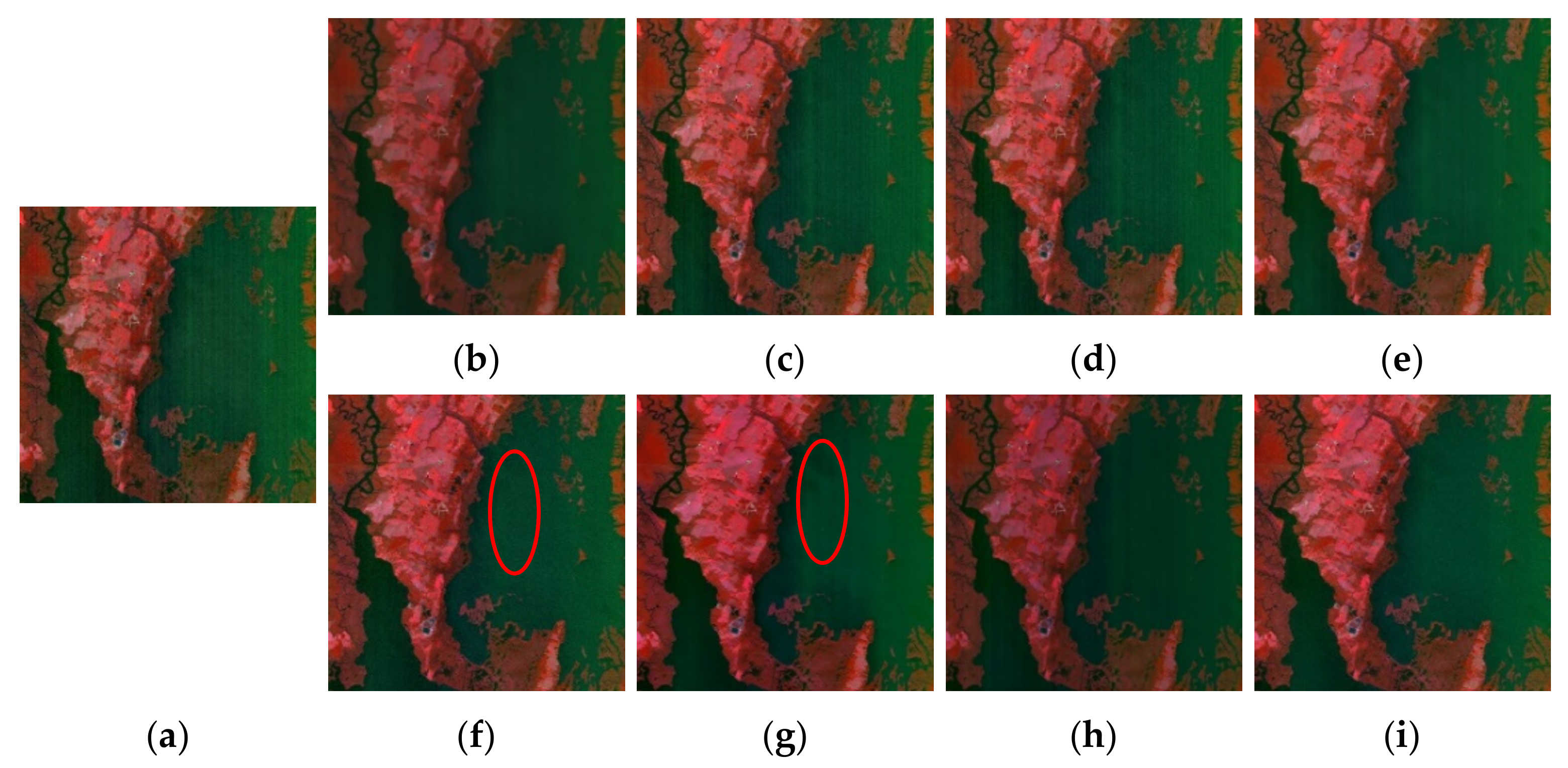
3.3.2. Zhuhai-1 Dataset

The Zhuhai-1 data had considerable stripe noise. We selected two scenes of size 512 × 512 as the experimental data. The stripes in scene 1 have different lengths and random widths, while the distribution is relatively sparse. These features meet the requirement for the method evaluation. The experimental results show (Figure 11) that the contrast method used in this study has varying degrees of inhibition on the stripes; some stripes remain. After the LRTV processing, numerous stripes remain. Meanwhile, LRMR, TDL, and NGMeet are not sufficiently stringent for stripe processing, as shown in Figure 11b–e. The ASSTV can suppress a part of the stripe, but stripes which are too intense exert only minor positive effect, while some portion of the stripe remains. The HSI-DeNet can effectively remove most stripes, but the loss of details and excessive smoothness emerge as a drawback. The SGIDN can inhibit a part of the stripe but cannot completely remove stripe noise, as shown in Figure 11h. After the TRS-DCHC processing, almost all stripe noise can be removed, while the original spatial and spectral information is better preserved.

For scene 2, a small and dense stripe is shown in Figure 12. Most parts of this stripe are hidden in the background and indistinguishable. LRTV efficiently removes most stripes, and it also leads to the loss of spectral information. LRMR and TDL cannot achieve a good processing effect on scene 2, and many stripes remain, as shown in Figure 12b–d. For NGMeet, a portion of the stripe is suppressed, but it is not sufficiently stringent given the emerged interference from the stripe. For ASSTV, most of the stripe can be removed well and the spectral information can be better preserved. However, there are some dense and small stripe residues, as demonstrated in Figure 12f. Figure 12g shows that HSI-DeNet removes stripes, but causes spectral loss. Similarly, SGIDN has a strong removal effect on stripe noise in scene 2, but some spectral loss inevitably occurs, as indicated by Figure 12h. TRS-DCHC can achieve better results, and the spectral information of the restored image is retained to a greater extent.

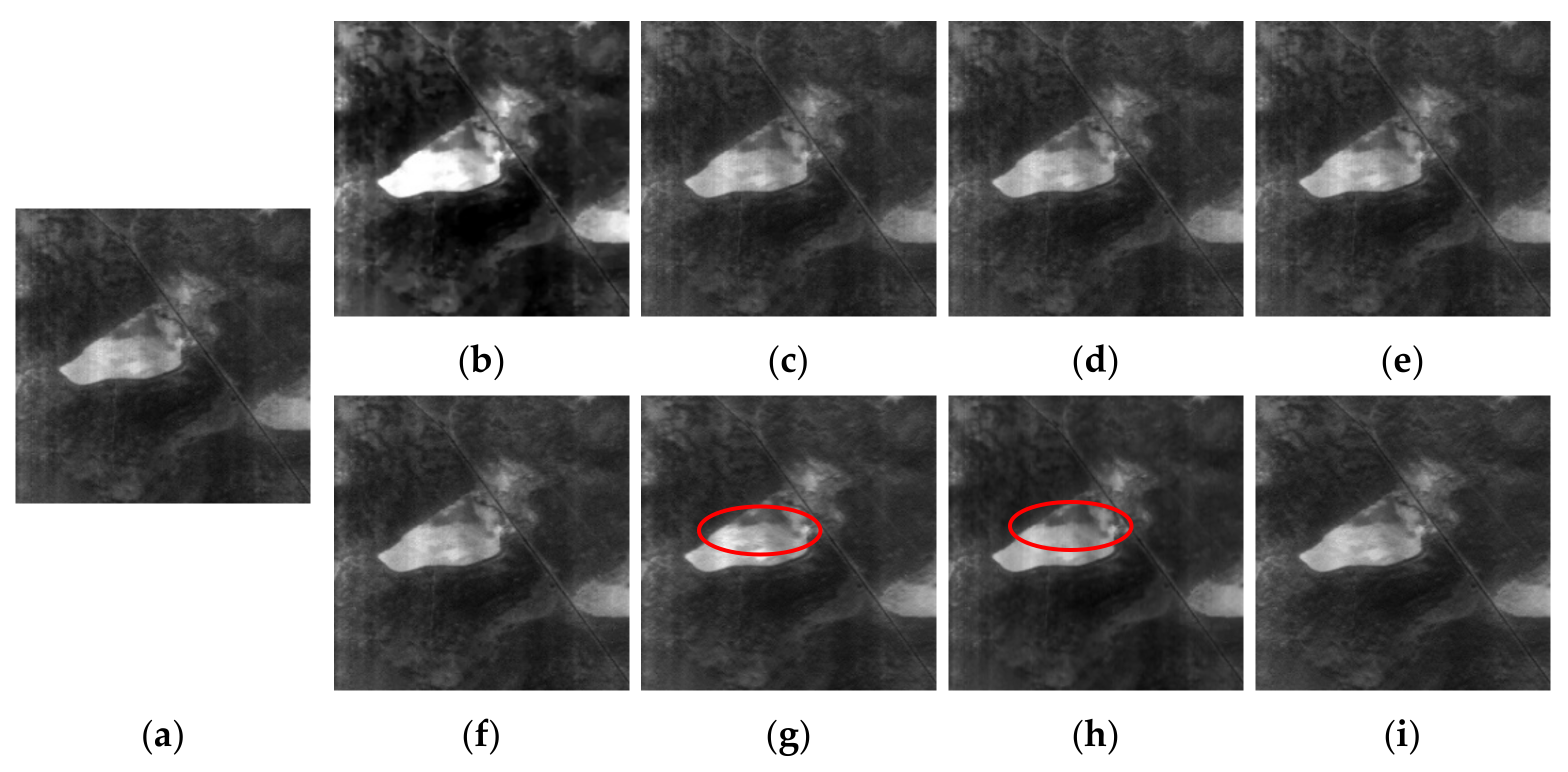
3.3.3. Hyperion EO-1 Dataset

The Hyperion EO-1 data have considerable stripe noise, random noise, and dead lines. The size of our experimental data was 200 × 200 × 210. The LRTV method still yields a considerably large area of residual noise, as shown in Figure 13b. LRMR and TDL have a certain significant effect on random noise, but the removal effect on stripe noise and dead lines is unsatisfactory, as indicated by Figure 13c,d. NGMeet can remove large-scale interference factors to a large extent, with only a small amount of unremoved noise, as shown in Figure 13e. Figure 13f illustrates that the ASSTV method has a good suppression effect on stripe noise and dead lines, but its ability to remove random noise is limited. As clearly indicated by Figure 13g, HSI-DeNet can remove nearly all noise, but it inevitably triggers smoothness-related problems. Similarly, SGIDN suffers from a severe over-smoothing problem, and the repair of the dead line interference area is incomplete, as shown in Figure 13h. Figure 13i illustrates the TRS-DHC good performance, where stripe noise, random noise, and dead lines are removed.

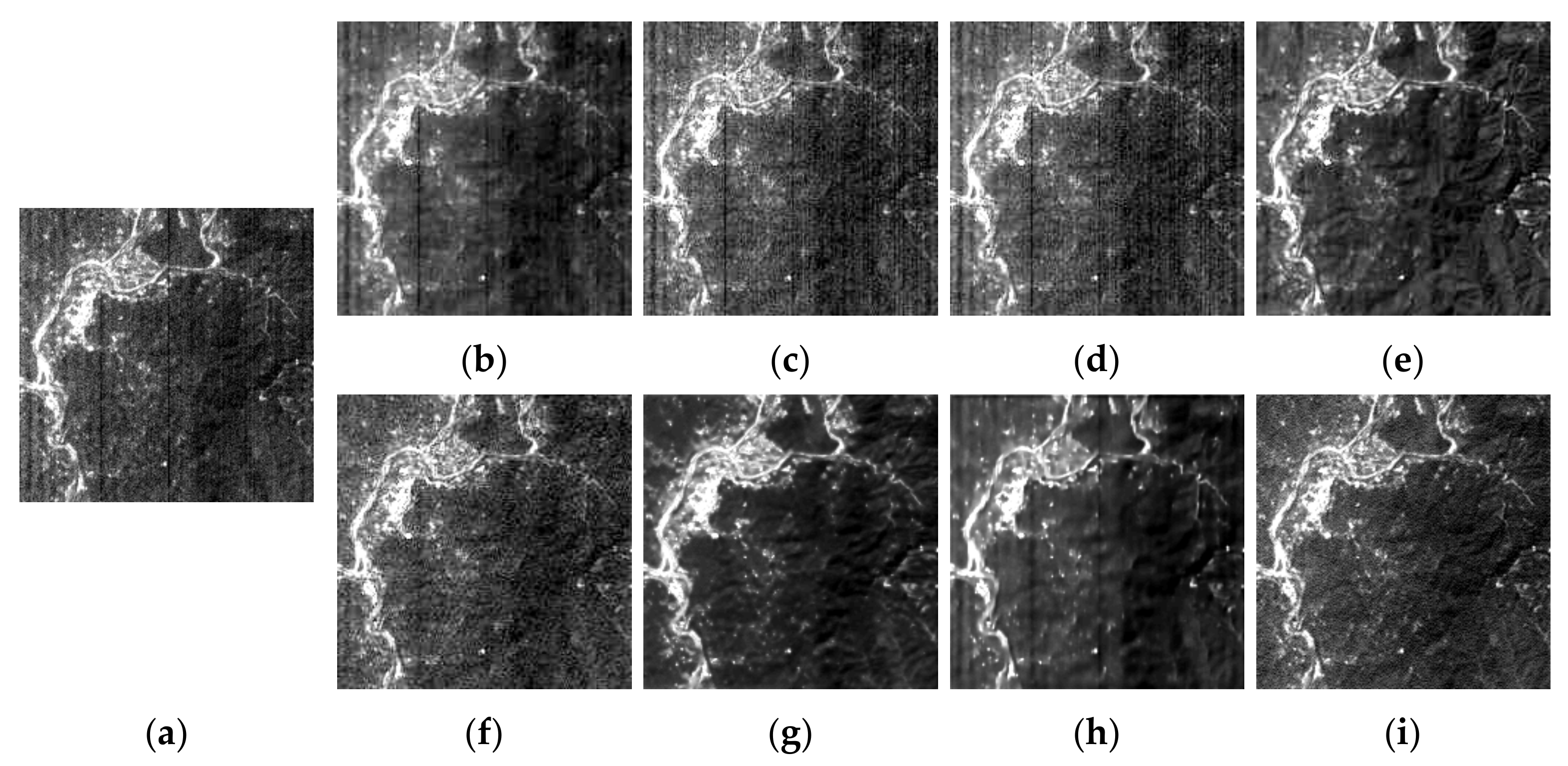
3.3.4. HYDICE Urban Data Set

The experimental data measured 306 × 306 × 210; the degradation factors were mainly stripe and Gaussian noise. The stripe removal results for band 1 are shown in Figure 14. In particular, Figure 14b clearly shows that the LRTD cannot completely remove stripe noise. Although LRMR can suppress only a portion of the stripe noise, it triggers a loss of some details (see Figure 14c). Similarly, Figure 14d shows that the TDL can have a certain effect on stripe removal, but the effect is ambiguous. The NGMeet can effectively remove stripe noise, but the spectral information of some ground features is lost. It exhibits over-smoothing to some extent, as shown in Figure 14e. After the ASSTV process, the stripes can be strongly suppressed, but they are not completely removed as displayed in Figure 14f. For HSI-DeNet, although stripe noise can be completely removed, it causes more serious loss of spatial information. Notably, the houses and road structures in the upper left are greatly smoothed, which is different from the original structure, as shown in Figure 14g. Similarly, the SGIDN removes most of the stripes, but triggers the loss of the ground structure, as indicated by Figure 14h. By contrast, the TRS-DCHC provides notably satisfactory results as it can completely remove stripe noise, while the original features and structure are better preserved.

The experimental results of real data indicate that LRTV, LRMR, TDL, NGMeet, and ASSTV can achieve destriping performance more or less on real stripe contained data. However, the selection of parameters during the experiment directly affects the destriping performance. The optimal parameters are more difficult to determine, and most of them use empirical values. For instance, if the parameters required by the LRTV were too low, the stripe removal performance would not be satisfactory. If it is set too high, it will damage the spectral and structural information and will directly affect the destriped result. It is difficult to achieve a balance between stripe removal and retention of spectral information. Despite the deep learning methods represented by HSI-DeNet and SGIDN that have strong feature extraction and learning capabilities, the stripe performance is not sufficiently stable. It exhibited variable processing capabilities driven by the type of data with emerged stripes. The TRS-DCHC method can process a wide range of different forms and types of noise. It is important to note that this study incorporates stripe noise derived from real data in the model training process, which is more complicated and sophisticated than Gaussian distributed noise. This incorporation strengthens the model capabilities for noise removal regardless of the type of noise. Our results provide the evidence that it was beneficial to use real data noise in model training.

4. Discussion

The TRS-DCHC utilizes a training strategy that combines real and simulated data and adds DWT to the network to explicitly decompose stripe patterns and stripe-free patterns, which is beneficial for improving the destriping performance. In this section, we conduct experiments while discussing and analyzing the effectiveness of adding real data training and DWT to the improvement of TRS-DCHC destriping ability. Furthermore, we also analyze the direction constrained stripe adaptive unsupervised extraction subnetwork and computation time of the TRS-DCHC.

4.1. Effectiveness toward Real Data Training Strategy

As reported in Table 1 and Table 2, the DCHC have conspicuous destriping performance, but not good as TRS-DCHC. For a more intuitive discussion on whether we can improve the performance of the network in the actual application process after incorporating real data, we compare the destriping performances of DCHC and TRS-DCHC using another set of Zhuhai-1 data as the experimental input to evaluate the effectiveness of the real data training strategy. The results are shown in Figure 15. The experimental results indicate that both TRS-DCHC and DCHC can remove interference stripes very well, and can completely retain the stripe-free component, while the spectral and structural information is completely restored. However, the enlarged picture indicates that the recovery ability of TRS-DCHC is better than that of DCHC, especially in the homogeneous area. Moreover, the result of the TRS-DCHC is more rigorously restored, while the result of the DCHC has little noise interference. For a more elaborate comparison, Figure 16 shows the mean cross-profile of the destriping result. Furthermore, Figure 16b,c demonstrate that after the destriping, the reconstruction profile of the TRS-DCHC is smoother, and the horizontal mean cross-profile shows that the TRS-DCHC yields a more effective destriping result. The experimental results show that the DCHC can also destripe the processing of real data to some extent. At the same time, it also proves that the stripe patterns of the real data during the training process can enhance the model’s ability to process sophisticated stripe patterns. Thus, the model ability to destripe noise in the actual application process is evidently improved. Therefore, incorporating a real data strategy is certainly effective and has practical significance for improving the destriping effect.

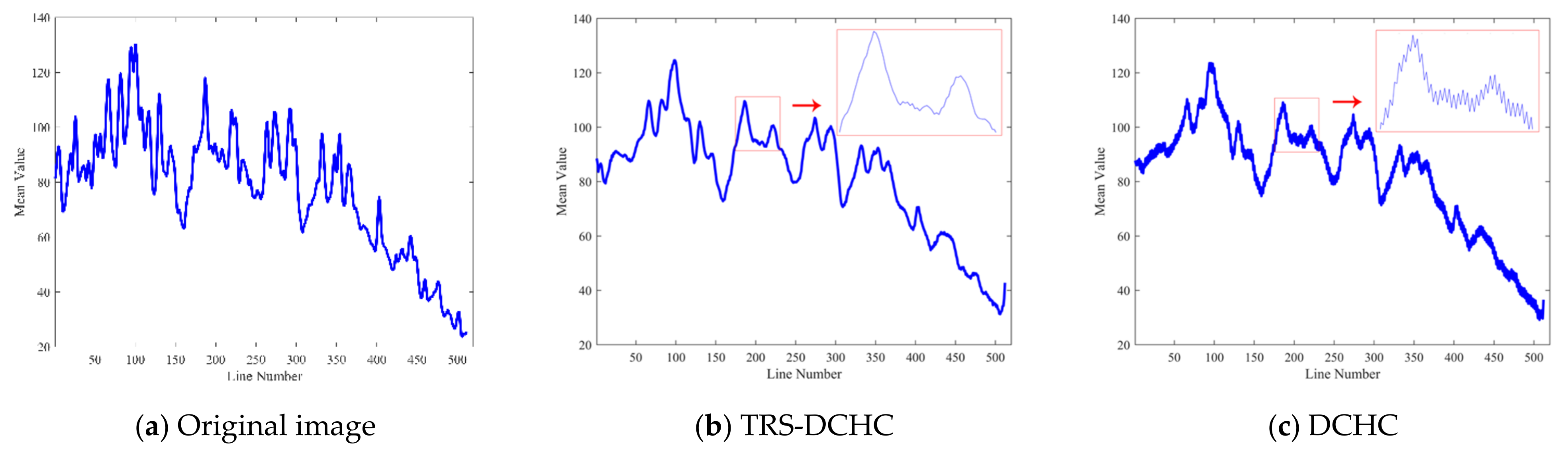
4.2. Effectiveness of DWT

Here, we discuss the influence of the DWT. The destriping performance of TRS-DCHC-noW in simulated, and real data are reported in Table 1 and Table 2. To evaluate the DWT positive effects on the destriping effect of the model and the recovery of spectral information, we use Case 2 in the simulation experiment as an example. Note that we refer to the model without DWT and IWT as TRS-DCHC-noW (Figure 17). The experimental results clearly show that both TRS-DCHC-noW and TRS-DCHC can remove stripe noise. However, the spectral information loss of the striped image of TRS-DCHC-noW was greater. By contrast, the TRS-DCHC preserves more complete spectral information. Figure 17e shows the pixel value in each band of the pixel at (100,100) and indicates that the result of TRC-DCHC is closer to the original pixel value. Based on this, we can deduce that adding DWT to CNN is beneficial for the destriping performance and for the repair effect of the model.

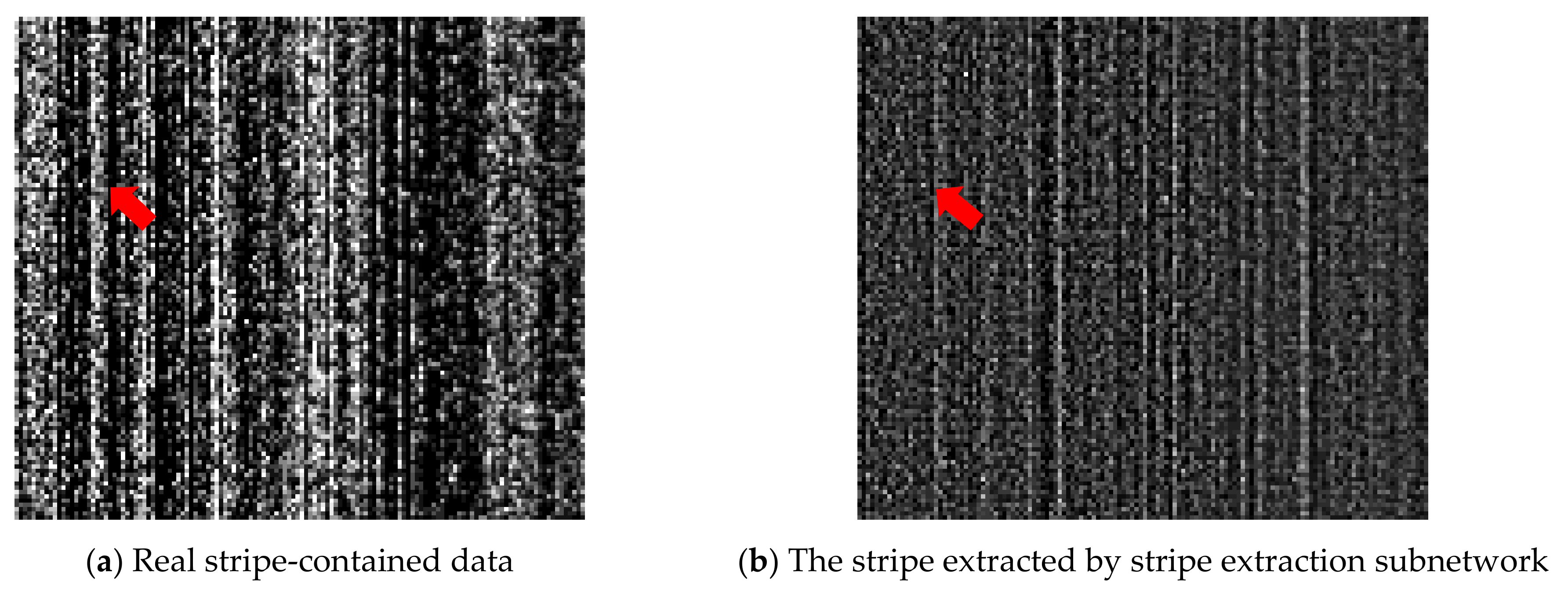
4.3. Analysis of Direction Constrained Stripe Adaptive Unsupervised Extraction Subnetwork

The stripe noise extracted from real stripe-contained data can improve the destriping performance of the TRS-DCHC as displayed in Section 4.1. In this section, we discuss the stripe extraction subnetwork. Figure 5 shown the stripe extracted from real data. Here, we use real data image for experiments and compare the output of the sub-network with real data, as shown in Figure 18. As shown in Figure 18, the spatial position distribution of the extracted noise is basically the same as that of the original noise, as shown by the red arrow, which shows that the sub-network has good strip noise extraction ability.

4.4. The Time Costs

This section compares the destriping time costs of different methods. All experiments were performed on a PC with Windows 10, 32 GB RAM, and an NVIDIA GeForce gtx2080 Ti GPU. Here, Case 2 from the simulation data experiment is taken as an example for the analysis. The size of the data is 200 × 200 × 191, and the time costs of each method are displayed in

Table 4. Time costs of difference destriping methods.

	Methods
	LRTV	LRMR	TDL	NGMeet	ASSTV	HSI-DeNet	SGIDN	TRS-DCHC
Time costs (s)	35.7	74.4	21.3	46.7	23.6	4.6	8.4	8.2

. According to Table 4, we can see the deep learning-based methods have lower time cost than traditional methods. The HSI-DeNet takes the least time, the TRS-DCHC method consumes the almost same time as the SGIDN method.

5. Conclusions

In this study, we proposed a novel method, namely a multi-scale hierarchical feature cascade network for HSI data destriping, that adopts stripe noise extracted from real data for model training. Our method is composed of two subnetworks: a direction-constrained stripe adaptive unsupervised extraction subnetwork, and a wavelet-based hierarchical feature cascaded destriping subnetwork. The stripe extraction subnetwork, which uses direction constraints to extrapolate stripe patterns from the local to the global, is utilized to extract the intrinsic stripe noise for real stripe-contaminated spaceborne hyperspectral imaging data. Notably, the extracted stripe noise was not generated by a noise generation model with a known distribution. Its statistical distribution and noise structure were diverse, complex, and unknown. The wavelet-based hierarchical feature cascaded destriping subnetwork explicitly decomposed stripe and stripe-free components by DWT to reduce the information loss of stripe-free components. Note that dense connection and hierarchical feature fusion were applied to minimize the information loss and integrate different levels of feature semantics. Both aspects improved the stripe removal effect. We used a variety of simulations and multiple sets of real satellite data with different loads and confirmed that the proposed method has superior performance in stripe suppression and image repair compared with previous methods. We also showed that in contrast to the single stripe generation method, adding stripe noise to the training data is beneficial for the stripe removal performance of the model. As a result, the model efficiently processes the various stripe types in real data. However, the performance of the TRS-DCHC still has some shortcomings that need to be further studied and resolved. In particular, future studies should focus on how to improve the precision and controllability of the stripe extraction subnetwork. In future studies, an unsupervised method can be used to enable the stripe extraction subnetwork to achieve the most efficient destriping and image restoration.

References

1. Yu, C.; Han, R.; Song, M.; Liu, C.; Chang, C.-I. Feedback attention-based dense CNN for hyperspectral image classification. IEEE Trans. Geosci. Remote Sens. 2021, 1–16. [Google Scholar] [CrossRef]
2. Sun, X.; Qi, Y.; Gao, L.; Sun, X.; Qi, H.; Zhang, B.; Shen, T. Ensemble-based information retrieval with mass estimation for hyperspectral target detection. IEEE Trans. Geosci. Remote Sens. 2021, 1–23. [Google Scholar] [CrossRef]
3. Zhang, X.; Sun, Y.; Shang, K.; Zhang, L.; Wang, S. Crop classification based on feature band set construction and object-oriented approach using hyperspectral images. IEEE J. Sel. Topics Appl. Earth Observ. Remote Sens. 2016, 9, 4117–4128. [Google Scholar] [CrossRef]
4. Song, M.; Shang, X.; Chang, C.-I. 3-D receiver operating characteristic analysis for hyperspectral image classification. IEEE Trans. Geosci. Remote Sens. 2020, 58, 8093–8115. [Google Scholar] [CrossRef]
5. Zhang, Q.; Yuan, Q.; Li, J.; Sun, F.; Zhang, L. Deep spatio-spectral Bayesian posterior for hyperspectral image non-i.i.d. noise removal. ISPRS J. Photogramm. Remote Sens. 2020, 164, 125–137. [Google Scholar] [CrossRef]
6. Wan, Y.; Ma, A.; He, W.; Zhong, Y. Accurate multi-objective low-rank and sparse model for hyperspectral image denoising method. IEEE Trans. Evol. Comput. 2021. [Google Scholar] [CrossRef]
7. Zhang, H.; Liu, L.; He, W.; Zhang, L. Hyperspectral with image denoising total variation regularization and nonlocal low-rank tensor decomposition. IEEE Trans. Geosci. Remote Sens. 2020, 58, 3071–3084. [Google Scholar] [CrossRef]
8. Zheng, Y.-B.; Huang, T.-Z.; Zhao, X.-L.; Chen, Y.; He, W. Double-factor-regularized low-rank tensor factorization for mixed noise removal in hyperspectral image. IEEE Trans. Geosci. Remote Sens. 2020, 58, 8450–8464. [Google Scholar] [CrossRef]
9. Zhuang, L.; Fu, X.; Ng, M.K.; Bioucas-Dias, J.M. Hyperspectral image denoising based on global and nonlocal low-rank factorizations. IEEE Trans. Geosci. Remote Sens. 2020. [Google Scholar] [CrossRef]
10. Zhang, H.; Cai, J.; He, W.; Shen, H.; Zhang, L. Double low-rank matrix decomposition for hyperspectral image denoising and destriping. IEEE Trans. Geosci. Remote Sens. 2021. [Google Scholar] [CrossRef]
11. Fan, H.; Li, C.; Guo, Y.; Kuang, G.; Ma, J. Spatial-spectral total variation regularized low-rank tensor decomposition for hyperspectral image denoising. IEEE Trans. Geosci. Remote Sens. 2018, 56, 6196–6213. [Google Scholar] [CrossRef]
12. Ye, M.; Qian, Y.; Zhou, J. Multitask sparse nonnegative matrix factorization for joint spectral-spatial hyperspectral imagery denoising. IEEE Trans. Geosci. Remote Sens. 2015, 53, 2621–2639. [Google Scholar] [CrossRef] [Green Version]
13. Rasti, B.; Sveinsson, J.R.; Ulfarsson, M.O.; Benediktsson, J.A. Hyperspectral image denoising using first order spectral roughness penalty in wavelet domain. IEEE J. Sel. Topics Appl. Earth Observ. Remote Sens. 2014, 7, 2458–2467. [Google Scholar] [CrossRef]
14. Chen, Y.; He, W.; Yokoya, N.; Huang, T.; Zhao, X. Nonlocal tensor-ring decomposition for hyperspectral image denoising. IEEE Trans. Geosci. Remote Sens. 2020, 58, 1348–1362. [Google Scholar] [CrossRef]
15. Wei, W.; Zhang, L.; Jiao, Y.; Tian, C.; Wang, C.; Zhang, Y. Intracluster structured low-rank matrix analysis method for hyperspectral denoising. IEEE Trans. Geosci. Remote Sens. 2019, 57, 866–880. [Google Scholar] [CrossRef]
16. Liu, N.; Li, W.; Tao, R.; Fowler, J.E. Wavelet-domain low-rank/group-sparse destriping for hyperspectral imagery. IEEE Trans. Geosci. Remote Sens. 2019, 57, 10310–10321. [Google Scholar] [CrossRef]
17. Wang, M.; Wang, Q.; Chanussot, J.; Li, D. Hyperspectral image mixed noise removal based on multidirectional low-rank modeling and spatial-spectral total variation. IEEE Trans. Geosci. Remote Sens. 2021, 59, 488–507. [Google Scholar] [CrossRef]
18. Othman, H.; Qian, S.-E. Noise reduction of hyperspectral imagery using hybrid spatial-spectral derivative-domain wavelet shrinkage. IEEE Trans. Geosci. Remote Sens. 2006, 44, 397–408. [Google Scholar] [CrossRef]
19. Rasti, B.; Sveinsson, J.R.; Ulfarsson, M.O. Wavelet-based sparse reduced-rank regression for hyperspectral image restoration. IEEE Trans. Geosci. Remote Sens. 2014, 52, 6688–6698. [Google Scholar] [CrossRef]
20. Chen, G.; Qian, S. Denoising of hyperspectral imagery using principal component analysis and wavelet shrinkage. IEEE Trans. Geosci. Remote Sens. 2011, 49, 973–980. [Google Scholar] [CrossRef]
21. Song, J.; Jeong, J.-H.; Park, D.-S.; Kim, H.-H.; Seo, D.-C.; Ye, J.C. Unsupervised denoising for satellite imagery using wavelet directional CycleGAN. IEEE Trans. Geosci. Remote Sens. 2021, 59, 6823–6839. [Google Scholar] [CrossRef]
22. Cao, X.; Fu, X.; Xu, C.; Meng, D. Deep spatial-spectral global reasoning network for hyperspectral image denoising. IEEE Trans. Geosci. Remote Sens. 2021. [Google Scholar] [CrossRef]
23. Zhang, Q.; Yuan, Q.; Li, J.; Liu, X.; Shen, H.; Zhang, L. Hybrid noise removal in hyperspectral imagery with a spatial–spectral gradient network. IEEE Trans. Geosci. Remote Sens. 2019, 57, 7317–7329. [Google Scholar] [CrossRef]
24. Zhong, Y.; Li, W.; Wang, X.; Jin, S.; Zhang, L. Satellite-ground integrated destriping network: A new perspective for EO-1 Hyperion and Chinese hyperspectral satellite datasets. Remote Sens. Environ. 2020, 237, 111416. [Google Scholar] [CrossRef]
25. Maffei, A.; Haut, J.M.; Paoletti, M.E.; Plaza, J.; Bruzzone, L.; Plaza, A. A single model CNN for hyperspectral image denoising. IEEE Trans. Geosci. Remote Sens. 2020, 58, 2516–2529. [Google Scholar] [CrossRef]
26. Yuan, Y.; Ma, H.; Liu, G. Partial-DNet: A novel blind denoising model with noise intensity estimation for HSI. IEEE Trans. Geosci. Remote Sens. 2021. [Google Scholar] [CrossRef]
27. Wang, X.; Luo, Z.; Li, W.; Hu, X.; Zhang, L.; Zhong, Y. A self-supervised denoising network for satellite-airborne-ground hyperspectral imagery. IEEE Trans. Geosci. Remote Sens. 2021. [Google Scholar] [CrossRef]
28. Dong, W.; Wang, H.; Wu, F.; Shi, G.; Li, X. Deep Spatial–spectral representation learning for hyperspectral image denoising. IEEE Trans. Comput. Imag. 2019, 5, 635–648. [Google Scholar] [CrossRef]
29. Chang, Y.; Chen, M.; Yan, L.; Zhao, X.-L.; Li, Y.; Zhong, S. Toward universal stripe removal via wavelet-based deep convolutional neural network. IEEE Trans. Geosci. Remote Sens. 2020, 58, 2880–2897. [Google Scholar] [CrossRef]
30. Liu, W.; Lee, J. A 3-D atrous convolution neural network for hyperspectral image denoising. IEEE Trans. Geosci. Remote Sens. 2019, 57, 5701–5715. [Google Scholar] [CrossRef]
31. Chang, Y.; Yan, L.; Fang, H.; Zhong, S.; Liao, W. HSI-DeNet: Hyperspectral image restoration via convolutional neural network. IEEE Trans. Geosci. Remote Sens. 2019, 57, 667–682. [Google Scholar] [CrossRef]
32. Jiang, X.; Zhang, L.; Xu, M.; Zhang, T.; Lv, P.; Zhou, B.; Yang, X.; Pang, Y. Attention scaling for crowd counting. In Proceedings of the IEEE/CVF Conference on Computer Vision and Pattern Recognition (CVPR), Seattle, WA, USA, 13–19 June 2020; pp. 4705–4714. [Google Scholar]
33. Fu, J.; Liu, J.; Tian, H.; Li, Y.; Bao, Y.; Fang, Z.; Lu, H. Dual attention network for scene seg-mentation. In Proceedings of the IEEE/CVF Conference on Computer Vision and Pattern Recognition (CVPR), Long Beach, CA, USA, 16–20 June 2019; pp. 3146–3154. [Google Scholar]
34. Lu, M.; Li, Z.-N.; Wang, Y.; Pan, G. Deep attention network for egocentric action recognition. IEEE Trans. Image Process. 2019, 28, 3703–3713. [Google Scholar] [CrossRef]
35. Wang, Z.; Xu, J.; Liu, L.; Zhu, F.; Shao, L. RANet: Ranking attention network for fast video object segmentation. In Proceedings of the IEEE/CVF International Conference on Computer Vision (ICCV), Seoul, Korea, 27 October–2 November 2019; pp. 3977–3986. [Google Scholar]
36. Zhu, M.; Jiao, L.; Liu, F.; Yang, S.; Wang, J. Residual spectral-spatial attention network for hyperspectral image classification. IEEE Trans. Geosci. Remote Sens. 2021, 59, 449–462. [Google Scholar] [CrossRef]
37. Sun, H.; Zheng, X.; Lu, X. A supervised segmentation network for hyperspectral image classification. IEEE Trans. Image Process. 2021, 30, 2810–2825. [Google Scholar] [CrossRef] [PubMed]
38. Xiang, P.; Song, J.; Qin, H.; Tan, W.; Li, H.; Zhou, H. Visual attention and background subtraction with adaptive weight for hyperspectral anomaly detection. IEEE J. Sel. Topics Appl. Earth Observ. Remote Sens. 2021, 14, 2270–2283. [Google Scholar] [CrossRef]
39. Marinelli, D.; Bovolo, F.; Bruzzone, L. A novel change detection method for multitemporal hyperspectral images based on binary hyperspectral change vectors. IEEE Trans. Geosci. Remote Sens. 2019, 57, 4913–4928. [Google Scholar] [CrossRef]
40. Anwar, S.; Barnes, N. Real Image denoising with feature attention. In Proceedings of the IEEE/CVF International Conference on Computer Vision (ICCV), Seoul, Korea, 27 October–2 November 2019; pp. 3155–3164. [Google Scholar]
41. Shi, Q.; Tang, X.; Yang, T.; Liu, R.; Zhang, L. Hyperspectral image denoising using a 3-D attention denoising network. IEEE Trans. Geosci. Remote Sens. 2021, 59, 1–16. [Google Scholar] [CrossRef]
42. Hu, X.; Fu, C.-W.; Zhu, L.; Qin, J.; Heng, P.-A. Direction-aware spatial context features for shadow detection and removal. IEEE Trans. Pattern Anal. Mach. Intell. 2020, 42, 2795–2808. [Google Scholar] [CrossRef] [PubMed] [Green Version]
43. Rudin, L.; Osher, S.; Fatemi, E. Nonlinear total variation based noise removal algorithms. Physica D. 1992, 60, 259–268. [Google Scholar] [CrossRef]
44. Liu, L.; Liu, J.; Yuan, S.; Slabaugh, G.; Leonardis, A.; Zhou, W.; Tian, Q. Wavelet-based dual-branch network for image demoireing. In Proceedings of the IEEE/CVF European Conference on Computer Vision (ECCV), Glasgow, UK, 23–28 August 2020; Available online: https://arxiv.org/pdf/2007.07173.pdf (accessed on 12 December 2021).
45. Liu, P.; Zhang, H.; Zhang, K.; Lin, L.; Zuo, W. Multi-level wavelet-CNN for image restoration. In Proceedings of the IEEE/CVF Conference on Computer Vision and Pattern Recognition Workshop (CVPRW), Salt Lake City, UT, USA, 18–22 June 2018; pp. 773–782. [Google Scholar]
46. Liu, Y.; Ma, L.; Zhao, Y.; Wang, N.; Qian, Y.; Li, W.; Gao, C.; Qiu, S.; Li, C. A spectrum extension approach for radiometric calibration of the advanced hyperspectral imager aboard the Gaofen-5 Satellite. IEEE Trans. Geosci. Remote Sens. 2021. [Google Scholar] [CrossRef]
47. Si, M.; Tang, B.-H.; Li, Z.-L.; Nerry, F.; Zhang, X.; Shang, G. An artificial neuron network with parameterization scheme for estimating net surface shortwave radiation from satellite data under clear sky—Application to simulated GF-5 data set. IEEE Trans. Geosci. Remote Sens. 2021, 59, 4262–4272. [Google Scholar] [CrossRef]
48. Kingma, D.P.; Ba, J. Adam: A method for stochastic optimization. In Proceedings of the International Conference on Learning Representations (ICLR), San Diego, CA, USA, 7–9 May 2015; pp. 1–15. [Google Scholar]
49. Chang, Y.; Yan, L.; Fang, H.; Luo, C. Anisotropic spectral-spatial total variation model for multispectral remote sensing image destriping. IEEE Trans. Image Process. 2015, 24, 1852–1866. [Google Scholar] [CrossRef]
50. He, W.; Zhang, H.; Zhang, L.; Shen, H. Total-variation-regularized low-rank matrix factorization for hyperspectral image restoration. IEEE Trans. Geosci. Remote Sens. 2016, 54, 178–188. [Google Scholar] [CrossRef]
51. He, W.; Yao, Q.; Li, C.; Yokoya, N.; Zhao, Q. Non-local meets global: An integrated paradigm for hyperspectral denoising. In Proceedings of the IEEE/CVF Conference on Computer Vision and Pattern Recognition (CVPR), Long Beach, CA, USA, 16–20 June 2019; pp. 6861–6870. [Google Scholar]
52. Zhang, H.; He, W.; Zhang, L.; Shen, H.; Yuan, Q. Hyperspectral image restoration using low-rank matrix recovery. IEEE Trans. Geosci. Remote Sens. 2014, 52, 4729–4743. [Google Scholar] [CrossRef]
53. Peng, Y.; Meng, D.; Xu, Z.; Gao, C.; Yang, Y.; Zhang, B. Decomposable nonlocal tensor dictionary learning for multispectral image denoising. In Proceedings of the IEEE/CVF Conference on Computer Vision and Pattern Recognition (CVPR), Columbus, OH, USA, 23–28 June 2014; pp. 2949–2956. [Google Scholar]
54. Wang, Z.; Bovik, A.C.; Sheikh, H.R.; Simoncelli, E.P. Image quality assessment: From error visibility to structural similarity. IEEE Trans. Image Process. 2014, 13, 600–612. [Google Scholar] [CrossRef] [PubMed] [Green Version]
55. Bouali, M.; Ladjal, S. Toward optimal destriping of MODIS data using a unidirectional variational model. IEEE Trans. Geosci. Remote Sens. 2011, 49, 2924–2935. [Google Scholar] [CrossRef]
56. Shen, H.; Zhang, L. A MAP-based algorithm for destriping and inpainting of remotely sensed images. IEEE Trans. Geosci. Remote Sens. 2009, 47, 1492–1502. [Google Scholar] [CrossRef]
Figure 1. Flowchart of the proposed TRS-DCHC. RB denotes the residual block, DCSC denotes the direction constrained spatial context module, and MsRB denotes the multi-scale residual block.
Remotesensing 14 00467 g001
Figure 2. Flowchart of the proposed direction constrained stripe adaptive extraction subnetwork. The arrow box denotes the feature map extracted by image spatial recurrent neural network (IRNN). (a) Direction constrained stripe adaptive extraction subnetwork. (b) Direction constraint spatial context module (DCSC). (c) Spatial context aggregation residual block (SCARB). (d) Multi-direction awarded local to global module (MDL2G).
Remotesensing 14 00467 g002
Figure 3. Schematic illustration of the extraction of two-round IRNN architectural global contextual features in two stages using a local to global strategy.
Remotesensing 14 00467 g003
Figure 4. Illustration of DWT. (a) Degraded image, (b) Extraction results of the image in different coefficients after DWT. The upper left is LL, the lower left is HL, the upper right is LH, and the lower right is HH.
Remotesensing 14 00467 g004
Figure 5. (ad) GF-5 data used in this article for stripe pattern extraction; (eh) stripe patterns extracted from real stripe-contained data by direction constrained stripe adaptive unsupervised extraction subnetwork.
Remotesensing 14 00467 g005
Figure 6. Destriping result of Case 1 (period stripe noise).
Remotesensing 14 00467 g006
Figure 7. Destriping result of Case 2 (random stripe noise).
Remotesensing 14 00467 g007
Figure 8. Destriping result of Case 3 (mixed stripe noise).
Remotesensing 14 00467 g008
Figure 9. Destriped results on GF-5 of scenes 1 with false color image (band: 70, 15, 90). (a) Degraded image. (b) LRTV. (c) LRMR. (d) TDL. (e) NGMeet. (f) ASSTV. (g) HSI-DeNet. (h) SGIDN. (i) TRS-DCHC.
Remotesensing 14 00467 g009
Figure 10. Destriped results on GF-5 of scenes 2 with false color image (band: 140, 1, 60). (a) Degraded image. (b) LRTV. (c) LRMR. (d) TDL. (e) NGMeet. (f) ASSTV. (g) HSI-DeNet. (h) SGIDN. (i) TRS-DCHC.
Remotesensing 14 00467 g010
Figure 11. Destriped results on Zhuihai-1 of scenes 1. (a) Degraded image. (b) LRTV. (c) LRMR. (d) TDL. (e) NGMeet. (f) ASSTV. (g) HSI-DeNet. (h) SGIDN. (i) TRS-DCHC.
Remotesensing 14 00467 g011
Figure 12. Destriped results on Zhuihai-1 of scenes 2. (a) Degraded image. (b) LRTV. (c) LRMR. (d) TDL. (e) NGMeet. (f) ASSTV. (g) HSI-DeNet. (h) SGIDN. (i) TRS-DCHC.
Remotesensing 14 00467 g012
Figure 13. Destriped results on Hyperion EO-1 with band 2. (a) Degraded image. (b) LRTV. (c) LRMR. (d) TDL. (e) NGMeet. (f) ASSTV. (g) HSI-DeNet. (h) SGIDN. (i) TRS-DCHC.
Remotesensing 14 00467 g013
Figure 14. Destriped results on HYDICE Urban with band 1. (a) Degraded image. (b) LRTV. (c) LRMR. (d) TDL. (e) NGMeet. (f) ASSTV. (g) HSI-DeNet. (h) SGIDN. (i) TRS-DCHC.
Remotesensing 14 00467 g014
Figure 15. Results for effectiveness toward real data training strategy.
Remotesensing 14 00467 g015
Figure 16. Mean cross profile analysis. The horizontal axis shows the line number of the image, and the vertical axis denotes the mean intensity value of the image.
Remotesensing 14 00467 g016
Figure 17. Results for effectiveness of DWT.
Remotesensing 14 00467 g017
Figure 18. Results for direction constrained stripe adaptive unsupervised extraction subnetwork.
Remotesensing 14 00467 g018