
Detection of Surface Crevasses over Antarctic Ice Shelves Using SAR Imagery and Deep Learning Method

Abstract
:1. Introduction
2. Study Area and Data Set
2.1. Study Area
2.2. Sentinel-1 SAR Data
2.3. Auxiliary Data
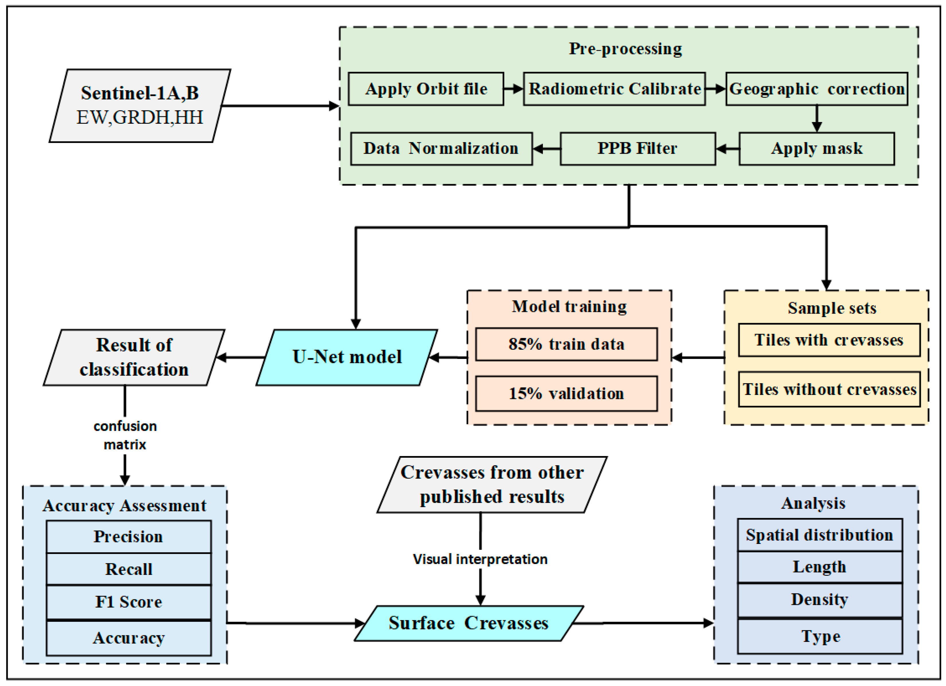
3. Methodology
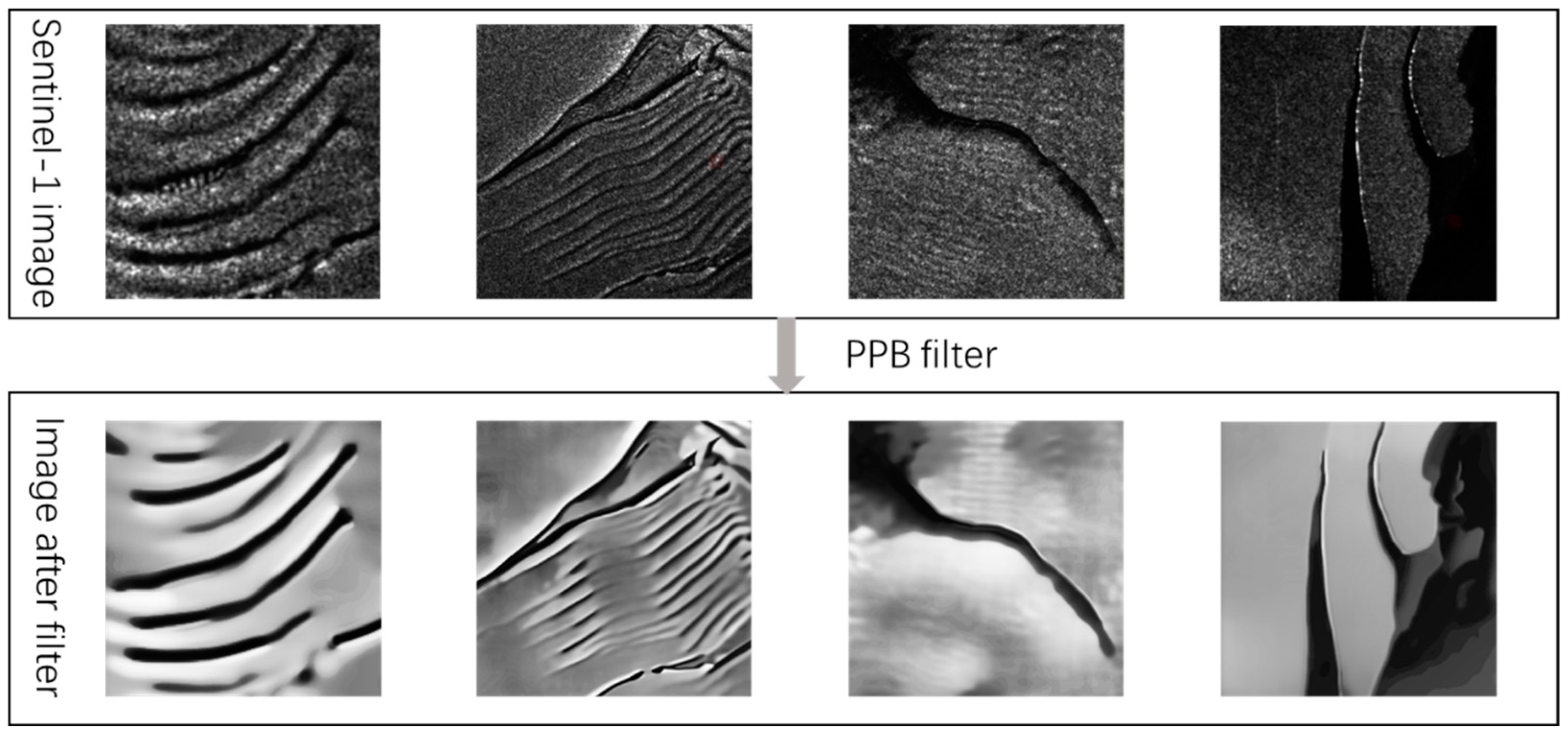
3.1. Pre-Processing and Data Preparation
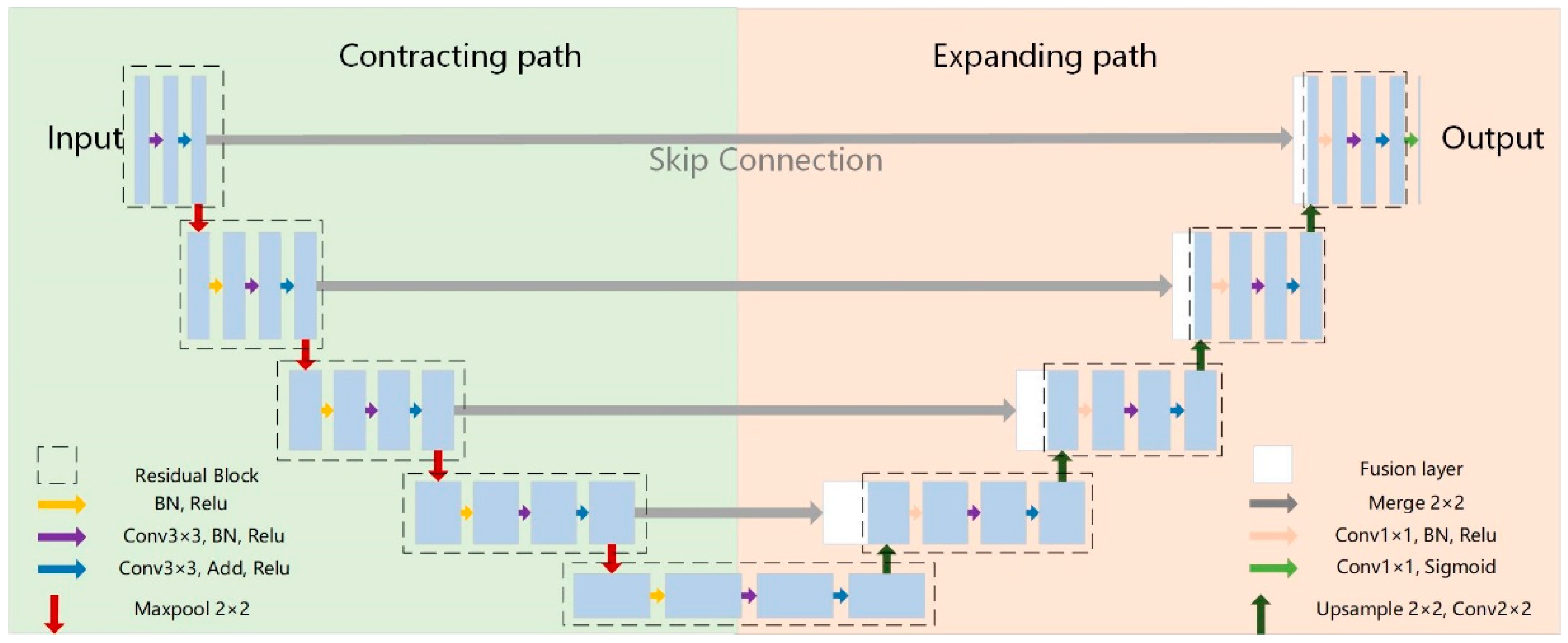
3.2. U-Net Architecture and Model Training
3.3. Accuracy Assessment
4. Results
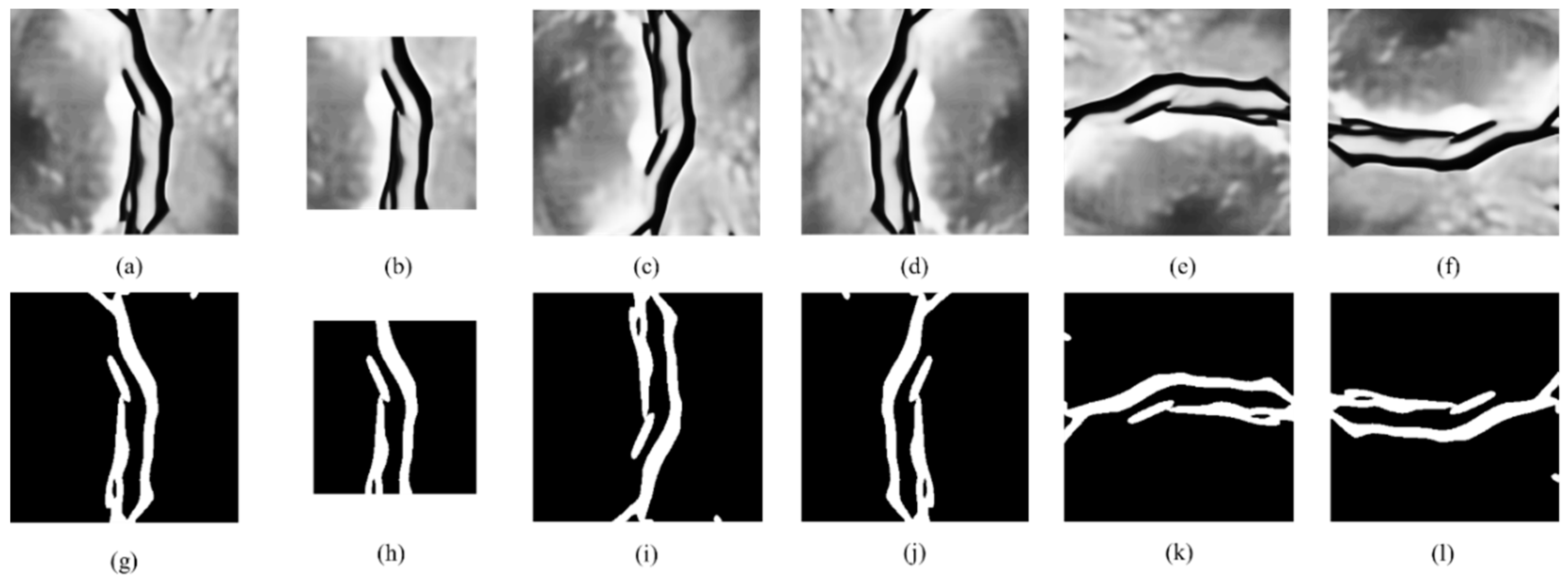
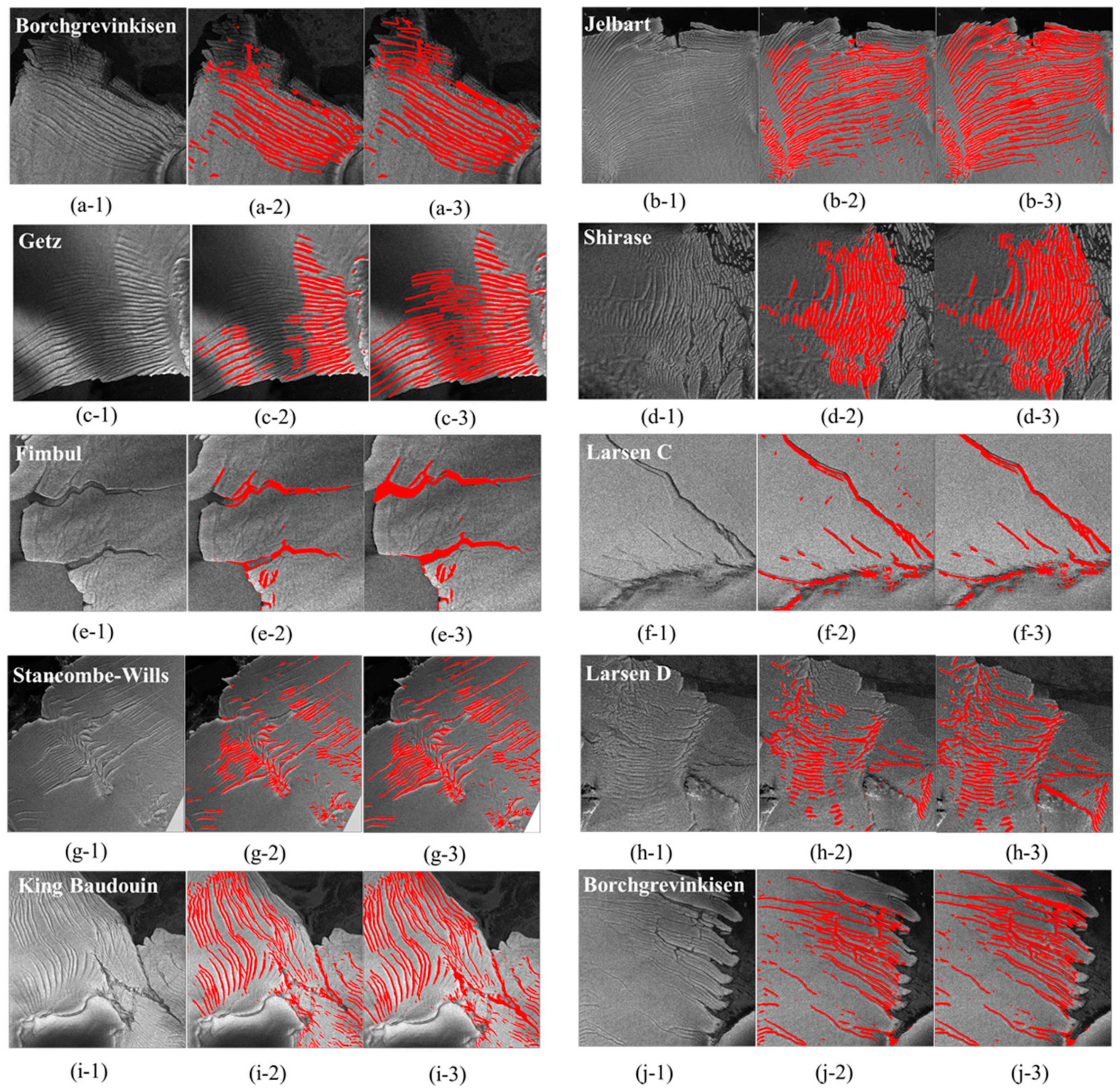
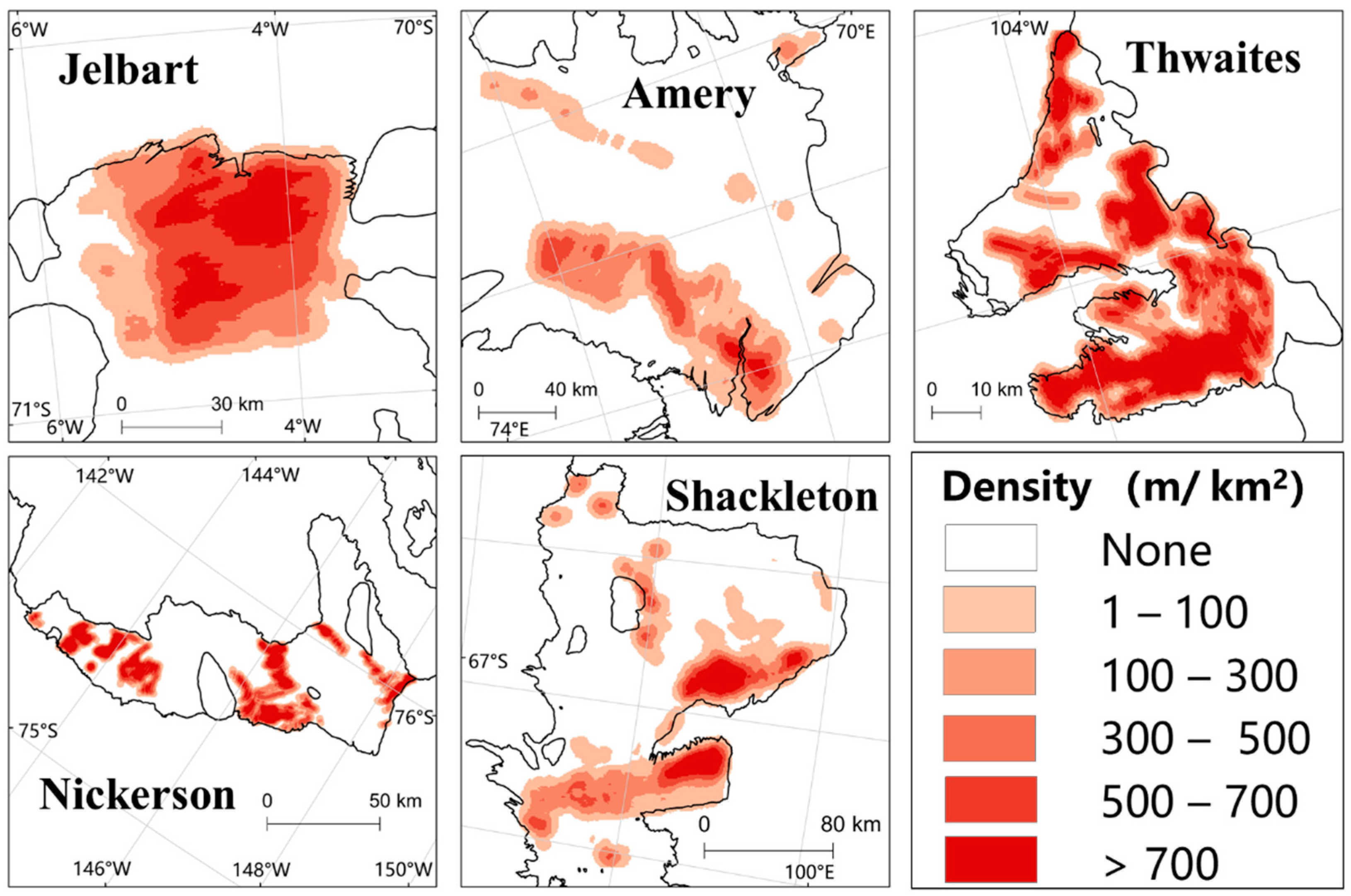
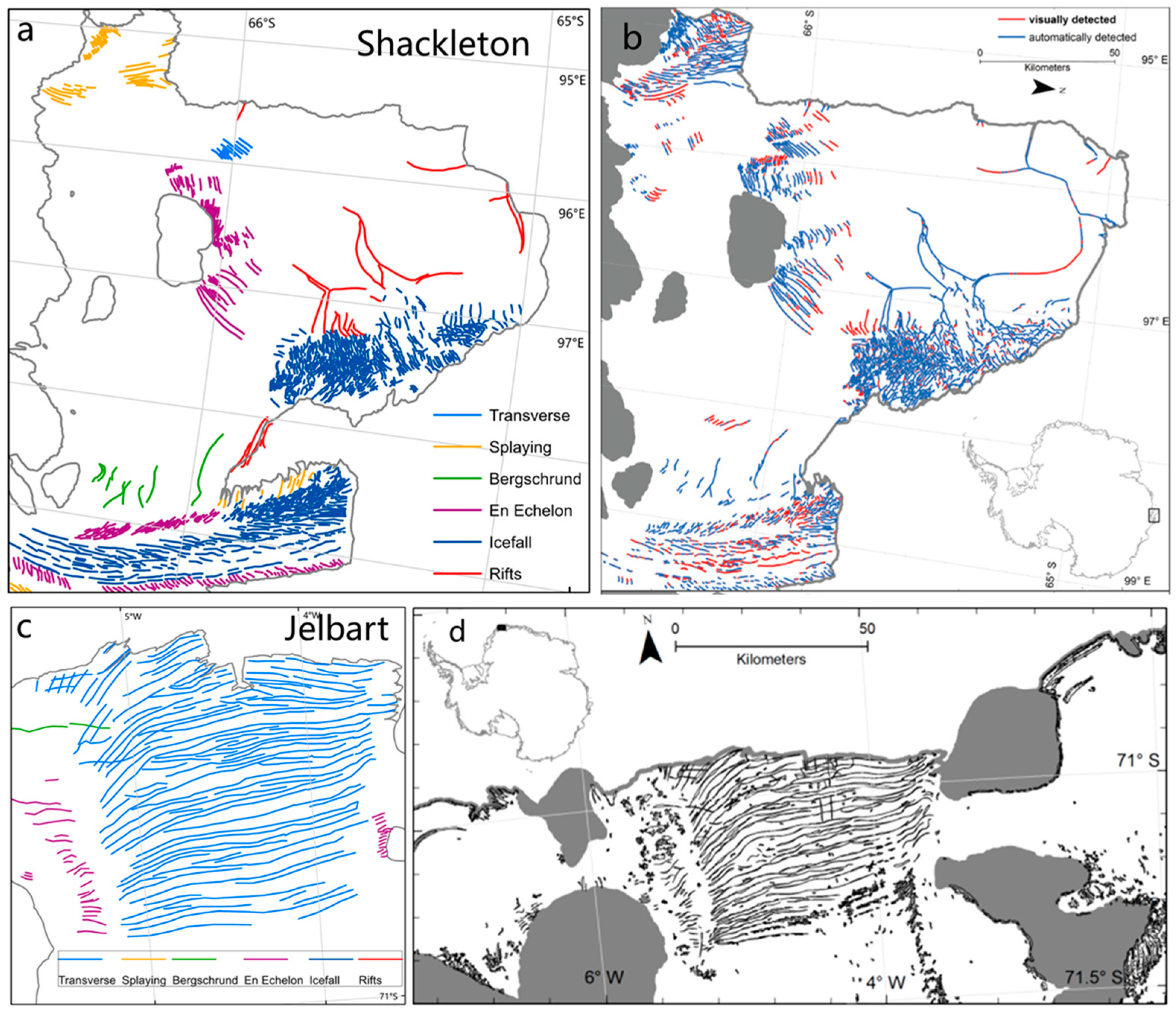
4.1. Crevasse Detection Result
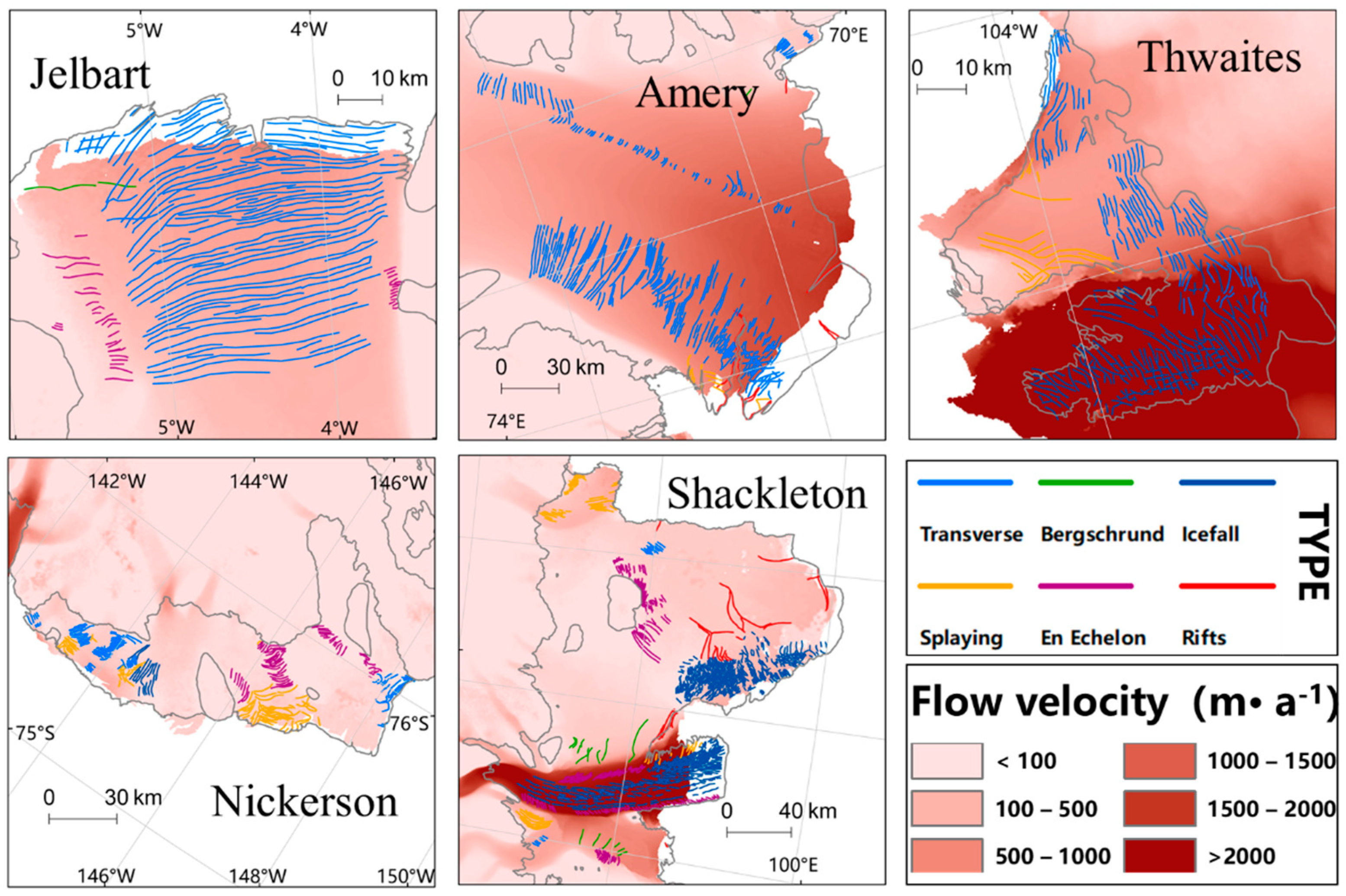
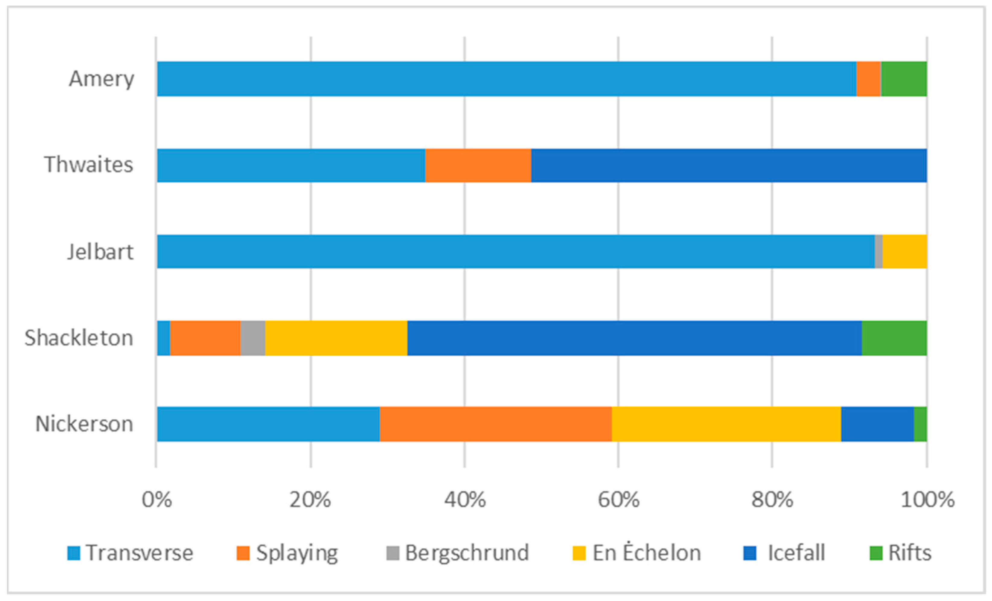
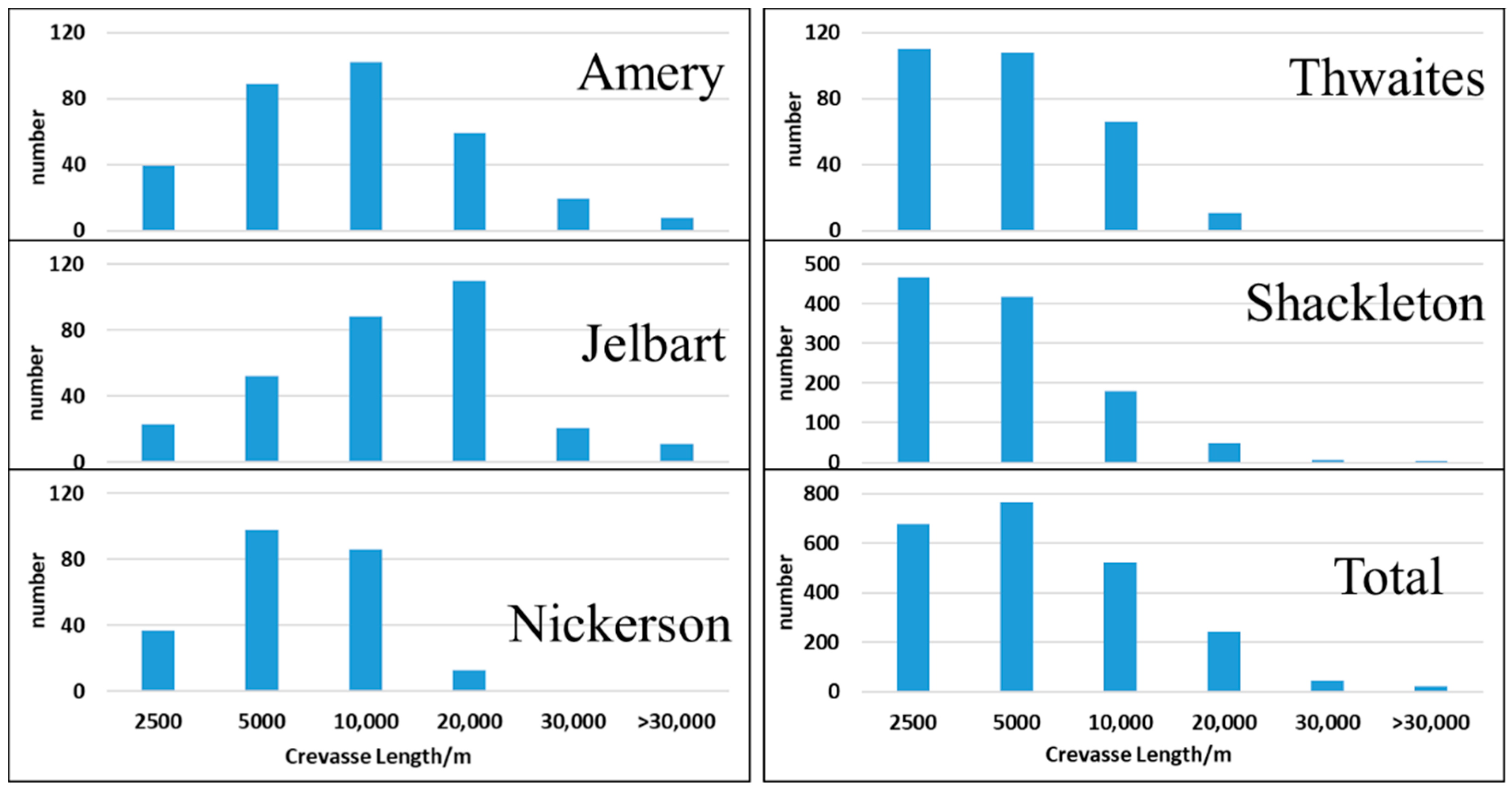
4.2. Analysis of Crevasse Characteristics
5. Discussion
6. Conclusions
Author Contributions
Funding
Institutional Review Board Statement
Informed Consent Statement
Data Availability Statement
Acknowledgments
Conflicts of Interest
References
- Colgan, W.; Rajaram, H.; Abdalati, W.; McCutchan, C.; Mottram, R.; Moussavi, M.S.; Grigsby, S. Glacier crevasses: Observations, models, and mass balance implications. Rev. Geophys. 2016, 54, 119–161. [Google Scholar] [CrossRef]
- Herzfeld, U.C.; Trantow, T.; Lawson, M.; Hans, J.; Medley, G. Surface heights and crevasse morphologies of surging and fast-moving glaciers from ICESat-2 laser altimeter data—Application of the density-dimension algorithm (DDA-ice) and evaluation using airborne altimeter and Planet Sky Sat data. Sci. Remote Sens. 2021, 3, 100013. [Google Scholar] [CrossRef]
- Miles, K.E.; Hubbard, B.; Irvine-Fynn, T.; Miles, E.S.; Rowan, A.V. Hydrology of debris-covered glaciers in High Mountain Asia. Earth-Sci. Rev. 2020, 207, 103212. [Google Scholar] [CrossRef]
- Gilbert, A.; Sinisalo, A.; Gurung, T.R.; Fujita, K.; Maharjan, S.B.; Sherpa, T.C.; Fukuda, T. The influence of water percolation through crevasses on the thermal regime of Himalayan Mountain glaciers. Cryosphere 2020, 14, 1273–1288. [Google Scholar] [CrossRef] [Green Version]
- Yang, K. The Progress of Greenland Ice Sheet Surface Ablation Research. J. Glaciol. Geocryol. 2013, 35, 101–109. [Google Scholar]
- Lai, C.Y.; Kingslake, J.; Wearing, M.G.; Chen, P.H.C.; Gentine, P.; Li, H.; van Wessem, J.M. Vulnerability of Antarctica’s ice shelves to meltwater-driven fracture. Nature 2019, 584, 574–578. [Google Scholar] [CrossRef]
- Thompson, S.S.; Cook, S.; Kulessa, B.; Winberry, J.P.; Fraser, A.D.; Galton-Fenzi, B.K. Comparing satellite and helicopter-based methods for observing crevasses, application in East Antarctica. Cold Reg. Sci. Technol. 2020, 178, 103128. [Google Scholar] [CrossRef]
- Whillans, I.M.; Merry, C.J. Analysis of a shear zone where a tractor fell into a crevasse, western side of the Ross Ice Shelf, Antarctica. Cold Reg. Sci. Technol. 2001, 33, 1–17. [Google Scholar] [CrossRef]
- Vornberger, P.L.; Whillans, I.M. Crevasse Deformation and Examples from Ice Stream B, Antarctica. J. Glaciol. 1990, 36, 3–10. [Google Scholar] [CrossRef] [Green Version]
- Delaney, A.J.; Arcone, S.A.; O’Bannon, A.; Wright, J. Crevasse detection with GPR across the Ross Ice Shelf, Antarctica. In Proceedings of the Tenth International Conference on Grounds Penetrating Radar, Delft, The Netherlands, 21–24 June 2004; pp. 777–780. [Google Scholar]
- Taurisano, A.; Tronstad, S.; Brandt, O.; Kohler, J. On the use of ground penetrating radar for detecting and reducing crevasse-hazard in Dronning Maud Land, Antarctica. Cold Reg. Sci. Technol. 2006, 45, 166–177. [Google Scholar] [CrossRef]
- Williams, R.M.; Ray, L.E.; Lever, J.H.; Burzynski, A.M. Crevasse Detection in Ice Sheets Using Ground Penetrating Radar and Machine Learning. IEEE J. Sel. Top. Appl. Earth Obs. Remote Sens. 2017, 7, 4836–4848. [Google Scholar] [CrossRef]
- Liu, Y.; Cheng, X.; Hui, F.; Wang, X.; Wang, F.; Cheng, C. Detection of crevasses over polar ice shelves using Satellite Laser Altimeter. Sci. China Earth Sci. 2014, 57, 1267–1277. [Google Scholar] [CrossRef]
- Bhardwaj, A.; Joshi, P.K.; Sam, L.; Singh, M.K.; Singh, S.; Kumar, R. Applicability of Landsat 8 data for characterizing glacier facies and supraglacial debris. Int. J. Appl. Earth Obs. Geoinf. 2015, 38, 51–64. [Google Scholar] [CrossRef]
- Merry, C.J.; Whillans, I.M. Ice-flow features on Ice Stream B, Antarctica, revealed by SPOT HRV imagery. J. Glaciol. 1993, 39, 515–527. [Google Scholar] [CrossRef] [Green Version]
- Moustafa, S.E.; Rennermalm, A.K.; Román, M.O.; Wang, Z.; Schaaf, C.B.; Smith, L.C.; Erb, A. Evaluation of satellite remote sensing albedo retrievals over the ablation area of the southwestern Greenland ice sheet. Remote Sens. Environ. 2017, 198, 115–125. [Google Scholar] [CrossRef]
- Colgan, W.; Steffen, K.; McLamb, W.S.; Abdalati, W.; Rajaram, H.; Motyka, R.; Anderson, R. An increase in crevasse extent, West Greenland: Hydrologic implications. Geophys. Res. Lett. 2011, 38, 1–7. [Google Scholar] [CrossRef] [Green Version]
- Herzfeld, U.C.; Zahner, O. A connectionist-geostatistical approach to automated image classification, applied to the analysis of crevasse patterns in surging ice. Comput. Geoences 2001, 27, 499–512. [Google Scholar]
- Ewertowski, M.W.; Evans, D.J.; Roberts, D.H.; Tomczyk, A.M.; Ewertowski, W.; Pleksot, K. Quantification of historical landscape change on the foreland of a receding polythermal glacier, Hørbyebreen, Svalbard. Geomorphology 2019, 325, 40–54. [Google Scholar] [CrossRef] [Green Version]
- Liu, Y.; Moore, J.C.; Cheng, X.; Gladstone, R.M.; Bassis, J.N.; Liu, H.; Hui, F. Ocean-driven thinning enhances iceberg calving and retreat of Antarctic ice shelves. Proc. Natl. Acad. Sci. USA 2015, 112, 3263–3268. [Google Scholar] [CrossRef] [PubMed] [Green Version]
- Huang, R.; Jiang, L.; Wang, H.; Yang, B. A Bidirectional Analysis Method for Extracting Glacier Crevasses from Airborne LiDAR Point Clouds. Remote Sens. 2019, 11, 2373. [Google Scholar] [CrossRef] [Green Version]
- Enderlin, E.M.; Bartholomaus, T.C. Sharp contrasts in observed and modeled crevasse patterns at Greenland’s marine terminating glaciers. Cryosphere 2020, 14, 4121–4133. [Google Scholar] [CrossRef]
- Bhardwaj, A.; Sam, L.; Singh, S.; Kumar, R. Automated detection and temporal monitoring of crevasses using remote sensing and their implications in glacier dynamics. Ann. Glaciol. 2015, 57, 81–91. [Google Scholar] [CrossRef] [Green Version]
- Xiao, X.; Zhang, T.; Zhong, X.; Shao, W.; Li, X. Support vector regression snow-depth retrieval algorithm using passive microwave remote sensing data. Remote Sens. Environ. 2018, 210, 48–64. [Google Scholar] [CrossRef]
- Xiao, X.; Liang, S.; He, T.; Wu, D.; Pei, C.; Gong, J. Estimating fractional snow cover from passive microwave brightness temperature data using MODIS snow cover product over North America. Cryosphere 2021, 15, 835–861. [Google Scholar] [CrossRef]
- Gomez, R.; Arigony-Neto, J.; De Santis, A.; Vijay, S.; Jaña, R.; Rivera, A. Ice dynamics of union glacier from SAR offset tracking. Glob. Planet Chang. 2019, 174, 1–15. [Google Scholar] [CrossRef]
- Garbe, J.; Albrecht, T.; Levermann, A.; Donges, J.F.; Winkelmann, R. The hysteresis of the Antarctic Ice Sheet. Nature 2020, 585, 538–544. [Google Scholar] [CrossRef]
- Pandey, M.; NCPant Arora, D.; Gupta, R. A review of Antarctic ice sheet fluctuations records during Cenozoic and its cause-and-effect relation with the climatic conditions. Polar Sci. 2021, 30, 100720. [Google Scholar] [CrossRef]
- Dow, C.F.; Lee, W.S.; Greenbaum, J.S.; Greene, C.A.; Zappa, C.J. Basal channels drive active surface hydrology and transverse ice shelf fracture. Sci. Adv. 2018, 4, 7212. [Google Scholar] [CrossRef] [Green Version]
- Langley, K.; Von Deschwanden, A.; Kohler, J.; Sinisalo, A.; Matsuoka, K.; Hattermann, T.; Isaksson, E. Complex network of channels beneath an Antarctic ice shelf. Geophys. Res. Lett. 2014, 41, 1209–1215. [Google Scholar] [CrossRef]
- Luckman, A.; Jansen, D.; Kulessa, B.; King, E.C.; Sammonds, P.; Benn, D.I. Basal crevasses in Larsen C Ice Shelf and implications for their global abundance. Cryosphere 2012, 6, 113–123. [Google Scholar] [CrossRef] [Green Version]
- Pivot, F. C-Band SAR Imagery for Snow-Cover Monitoring at Tree line, Churchill, Manitoba, Canada. Remote Sens. 2012, 4, 2133–2155. [Google Scholar] [CrossRef] [Green Version]
- Marsh, O.J.; Price, D.; Courville, Z.R.; Floricioiu, D. Crevasse and rift detection in Antarctica from TerraSAR-X satellite imagery. Cold Reg. Sci. Technol. 2021, 187, 103284. [Google Scholar] [CrossRef]
- Benn, D.; Astrom, J. Calving glaciers and ice shelves. Adv. Phys. X 2018, 3, 1513819. [Google Scholar] [CrossRef] [Green Version]
- Cook, S.; Åström, J.; Zwinger, T.; Galton-Fenzi, B.K.; Greenbaum, J.S.; Coleman, R. Modelled fracture and calving on the Totten Ice Shelf. Cryosphere 2018, 12, 2401–2411. [Google Scholar] [CrossRef] [Green Version]
- Jacobel, R.W.; Christianson, K.; Wood, A.C.; Dallasanta, K.J.; Gobel, R.M. Morphology of basal crevasses at the grounding zone of Whillans Ice Stream, West Antarctica. Ann. Glaciol. 2014, 55, 57–63. [Google Scholar] [CrossRef] [Green Version]
- McGrath, D.; Steffen, K.; Scambos, T.; Rajaram, H.; Casassa, G.; Lagos, J.L.R. Basal crevasses and associated surface crevassing on the Larsen C ice shelf, Antarctica, and their role in ice-shelf instability. Ann. Glaciol. 2012, 53, 10–18. [Google Scholar] [CrossRef] [Green Version]
- Deledalle, C.; Denis, L.; Tupin, F. Iterative Weighted Maximum Likelihood Denoising with Probabilistic Patch-Based Weights. IEEE Trans. Image Process. 2009, 18, 2661–2672. [Google Scholar] [CrossRef] [Green Version]
- Li, R.; Liu, W.; Yang, L.; Sun, S.; Hu, W.; Zhang, F.; Li, W. DeepUNet: A Deep Fully Convolutional Network for Pixel-Level Sea-Land Segmentation. IEEE J. Sel. Top. Appl. Earth Obs. Remote Sens. 2018, 11, 3954–3962. [Google Scholar] [CrossRef] [Green Version]
- Hoeser, T.; Bachofer, F.; Kuenzer, C. Object Detection and Image Segmentation with Deep Learning on Earth Observation Data: A Review—Part II: Applications. Remote Sens. 2020, 12, 1667. [Google Scholar] [CrossRef]
- Dirscherl, M.; Dietz, A.J.; Kneisel, C.; Kuenzer, C. A Novel Method for Automated Supraglacial Lake Mapping in Antarctica Using Sentinel-1 SAR Imagery and Deep Learning. Remote Sens. 2021, 13, 197. [Google Scholar] [CrossRef]
- He, K.; Zhang, X.; Ren, S.; Sun, J. Deep residual learning for image recognition. In Proceedings of the IEEE Conference on Computer Vision and Pattern Recognition, Las Vegas, NV, USA, 27–30 June 2016; pp. 770–778. [Google Scholar]
- Glorot, X.; Bordes, A.; Bengio, Y. Deep sparse rectifier neural networks. In Proceedings of the Fourteenth International Conference on Artificial Intelligence and Statistics, Fort Lauderdale, FL, USA, 11–13 April 2011. [Google Scholar]
- Simonyan, K.; Zisserman, A. Very deep convolutional networks for large-scale image recognition. arXiv 2014, arXiv:1409.1556. [Google Scholar]
- Baumhoer, C.A.; Dietz, A.J.; Kneisel, C.; Kuenzer, C. Automated Extraction of Antarctic Glacier and Ice Shelf Fronts from Sentinel-1 Imagery Using Deep Learning. Remote Sens. 2019, 11, 2529. [Google Scholar] [CrossRef] [Green Version]
- Li, Q.J.; Zhao, Y.Q.; Gu, Z. Design of loss function for cost-sensitive learning. Control Theory Appl. 2015, 32, 689–694. [Google Scholar]
- Ronneberger, O.; Fischer, P.; Brox, T. U-Net: Convolutional Networks for Biomedical Image Segmentation. In Medical Image Computing and Computer-Assisted Intervention—MICCAI 2015; Springer International Publishing: Cham, Switzerland, 2015. [Google Scholar]
- Szegedy, C.; Vanhoucke, V.; Ioffe, S.; Shlens, J.; Wojna, Z. Rethinking the inception architecture for computer vision. In Proceedings of the IEEE Conference on Computer Vision and Pattern Recognition, Las Vegas, NV, USA, 27–30 June 2016; pp. 2818–2826. [Google Scholar]
- Nielsen, M.A. Neural Networks and Deep Learning; Determination Press: San Francisco, CA, USA, 2015; Volume 25. [Google Scholar]
- Mottram, R.; Benn, D. Testing crevasse-depth models: A field study at Breiðamerkurjökull, Iceland. J. Glaciol. 2009, 55, 746–752. [Google Scholar] [CrossRef] [Green Version]
- Cathles, L.M.; Abbot, D.S.; Bassis, J.N.; MacAyeal, D. Modeling surface-roughness/solar-ablation feedback: Application to small-scale surface channels and crevasses of the Greenland ice sheet. Ann. Glaciol. 2011, 52, 99–108. [Google Scholar] [CrossRef] [Green Version]
- Phillips, T.; Rajaram, H.; Steffen, K. Cryo-hydrologic warming: A potential mechanism for rapid thermal response of ice sheets. Geophys. Res. Lett. 2010, 37, L20503. [Google Scholar] [CrossRef]
- Poinar, K.; Joughin, I.; Lilien, D.; Brucker, L.; Kehrl, L.; Nowicki, S. Drainage of Southeast Greenland Firn Aquifer Water through Crevasses to the Bed. Front. Earth Sci. 2017, 5, 5. [Google Scholar] [CrossRef] [Green Version]
- Wesche, C.; Jansen, D.; Dierking, W. Calving Fronts of Antarctica: Mapping and Classification. Remote Sens. 2013, 5, 6305–6322. [Google Scholar] [CrossRef] [Green Version]
- Koike, K.; Yoshida, H.; Omura, M.; Shibuya, K.; Doi, K. Temporal changes in crevasses in the middle Slessor Glacier, Coats Land, East Antarctica through SAR data analysis. Earth Planets Space 2012, 64, 257–267. [Google Scholar] [CrossRef] [Green Version]
- Xiao, X.; He, T.; Liang, S.; Zhao, T. Improving fractional snow cover retrieval from passive microwave data using a radiative transfer model and machine learning method. IEEE Trans. Geosci. Remote Sens. 2021, 1. [Google Scholar] [CrossRef]


| ID | Time Period/Date | Orbit | Study Area | Region | Orbit Direction |
|---|---|---|---|---|---|
| Training regions | |||||
| 1 | 20200201T082024 | 31,056 | Wilkins Ice Shelf | API | Descending |
| 2 | 20200103T063435 | 30,632 | Ronne Ice Shelf | EAIS | Descending |
| 3 | 20200109T221939 | 30,729 | Riiser-Larsen Ice Shelf | EAIS | Ascending |
| 4 | 20200104T203224 | 30,655 | Fimbul Ice Shelf | EAIS | Ascending |
| 5 | 20200104T135847 | 30,651 | Amery Ice Shelf | EAIS | Ascending |
| 6 | 20200101T151212 | 30,608 | West Ice Shelf | EAIS | Ascending |
| 7 | 20200104T121959 | 30,650 | Totten Ice Shelf | EAIS | Ascending |
| 8 | 20200102T091714 | 30,619 | Aviator Ice Shelf | EAIS | Ascending |
| 9 | 20200105T080100 | 30,662 | Nickerson Ice Shelf | WAIS | Ascending |
| 10 | 20200102T041954 | 30,616 | Dotson Ice Shelf | WAIS | Ascending |
| Test regions | |||||
| 1 | 20200103T080958 | 30,633 | Larsen Ice Shelf | API | Descending |
| 2 | 20200111T233941 | 30,759 | Stancombe-Wills Ice Shelf | EAIS | Ascending |
| 3 | 20200129T193454 | 31,019 | Borchgrevinkisen Ice Shelf | EAIS | Ascending |
| 4 | 20200129T193558 | 31,019 | King Baudouin Ice Shelf | EAIS | Ascending |
| 5 | 20200130T183829 | 31,033 | Shirase Ice Shelf | EAIS | Ascending |
| 6 | 20200104T153739 | 30,652 | Amery Ice Shelf | EAIS | Ascending |
| 7 | 20200105T130231 | 30,665 | Shackleton Ice Shelf | EAIS | Ascending |
| 8 | 20200105T112334 | 30,664 | Holme Ice Shelf | EAIS | Ascending |
| 9 | 20200102T091514 | 30,619 | Ross Ice Shelf | WAIS | Ascending |
| 10 | 20200102T024259 | 30,615 | Venable Ice Shelf | WAIS | Ascending |
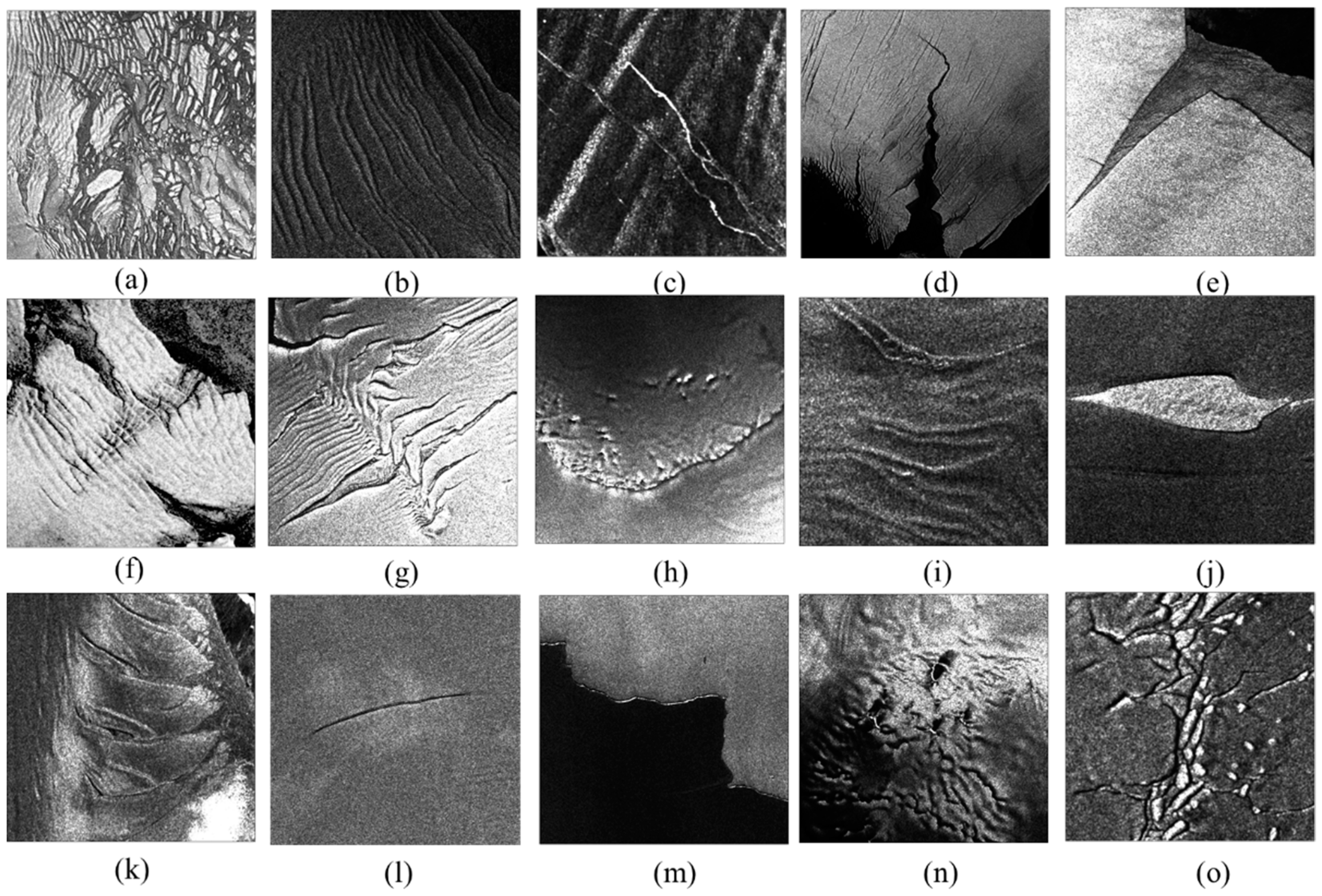
| Type of Crevasses | Dynamic Reasons | Image Recognition Signs |
|---|---|---|
| Transverse crevasse | The longitudinal tensile stress caused by the difference in the lateral velocity of the glacier surface has a large amount of longitudinal extension, which usually bulges on the downstream side. | It is manifested by the appearance of bright white lines (snow) or black lines (water filling), which are relatively regular and parallel to each other, perpendicular to the direction of glacier flow, and transverse to other features. |
| Splaying crevasse | It is caused by thrust faults, mainly under the condition of longitudinal compression, and secondly under the condition of lateral compression flow. | Commonly found near the glacier termini. Extends sideways along the direction of glacier flow. |
| Bergschrund, | Formed at the beginning of a glacier, the glacier pulls away from the rock wall at its head. | Usually located in the upper part of the glacier, a relatively independent single crevasse. |
| En échelon crevasses | Produced by the shear force between the valley wall and the glacier. It usually occurs at the turn of the glacier and is caused by the rotational strain of the shear zone. | It is usually located on the glacier valley wall, more closely spaced, with a certain curve, forming an angle from the valley wall to the top of the glacier. |
| Icefall | When the glacier flows on the convex bed, a series of crevasses are produced from the rupture of laminar flow. | Along the direction of glacier flow, it is common in accumulation areas and near steep slopes. |
| Rift | The edge of the ice shelf is deformed and bent due to tidal motion or the active glacier tributaries merged and applied a strong lateral shear force in the inactive area, resulting in crevasses. | The surface crevasses have a visible opening, usually oriented at a right angle to the direction of flow, deep enough to penetrate the entire thickness of the shelf. |
| Actual | Predicted | |
|---|---|---|
| Positive | Negative | |
| Positive | TP | FN |
| Negative | FP | TN |
| Images | Precision (%) | Recall (%) | F1 (%) | Accuracy (%) |
|---|---|---|---|---|
| Figure 8a (Borchgrevinkisen Ice Shelf) | 87.50 | 56.76 | 68.85 | 81.00 |
| Figure 8b (Jelbart Ice Shelf) | 77.08 | 80.43 | 78.72 | 80.00 |
| Figure 8c (Getz Ice Shelf) | 64.29 | 45.00 | 52.94 | 68.00 |
| Figure 8d (Shirase Ice Shelf) | 79.17 | 86.36 | 82.61 | 83.84 |
| Figure 8e (Fimbul Ice Shelf) | 76.92 | 58.82 | 66.67 | 90.00 |
| Figure 8f (Larsen C Ice Shelf) | 77.27 | 89.47 | 82.93 | 92.86 |
| Figure 8g (Stacombe-Wills Ice Shelf) | 94.44 | 91.89 | 93.15 | 95.00 |
| Figure 8h (Larsen D Ice Shelf) | 87.88 | 63.04 | 73.42 | 78.79 |
| Figure 8i (King Baudouin Ice Shelf) | 74.36 | 72.50 | 73.42 | 78.79 |
| Figure 8j (Borchgrevinkisen Ice Shelf) | 95.45 | 80.77 | 87.50 | 94.00 |
| Average | 81.44 | 72.50 | 76.02 | 84.23 |
| Locations | Amery | Thwaites | Jelbart | Shackleton | Nickerson |
|---|---|---|---|---|---|
| Length (m) | 8476 | 4075 | 11,300 | 3880 | 4922 |
| Density (m/km2) | 297 | 411 | 367 | 308 | 377 |
Publisher’s Note: MDPI stays neutral with regard to jurisdictional claims in published maps and institutional affiliations. |
© 2022 by the authors. Licensee MDPI, Basel, Switzerland. This article is an open access article distributed under the terms and conditions of the Creative Commons Attribution (CC BY) license (https://creativecommons.org/licenses/by/4.0/).
Share and Cite
Zhao, J.; Liang, S.; Li, X.; Duan, Y.; Liang, L. Detection of Surface Crevasses over Antarctic Ice Shelves Using SAR Imagery and Deep Learning Method. Remote Sens. 2022, 14, 487. https://doi.org/10.3390/rs14030487
Zhao J, Liang S, Li X, Duan Y, Liang L. Detection of Surface Crevasses over Antarctic Ice Shelves Using SAR Imagery and Deep Learning Method. Remote Sensing. 2022; 14(3):487. https://doi.org/10.3390/rs14030487
Chicago/Turabian StyleZhao, Jingjing, Shuang Liang, Xinwu Li, Yiru Duan, and Lei Liang. 2022. "Detection of Surface Crevasses over Antarctic Ice Shelves Using SAR Imagery and Deep Learning Method" Remote Sensing 14, no. 3: 487. https://doi.org/10.3390/rs14030487
APA StyleZhao, J., Liang, S., Li, X., Duan, Y., & Liang, L. (2022). Detection of Surface Crevasses over Antarctic Ice Shelves Using SAR Imagery and Deep Learning Method. Remote Sensing, 14(3), 487. https://doi.org/10.3390/rs14030487