
Insect-Equivalent Radar Cross-Section Model Based on Field Experimental Results of Body Length and Orientation Extraction


 ,
, 
Abstract
:
1. Introduction
- 1.
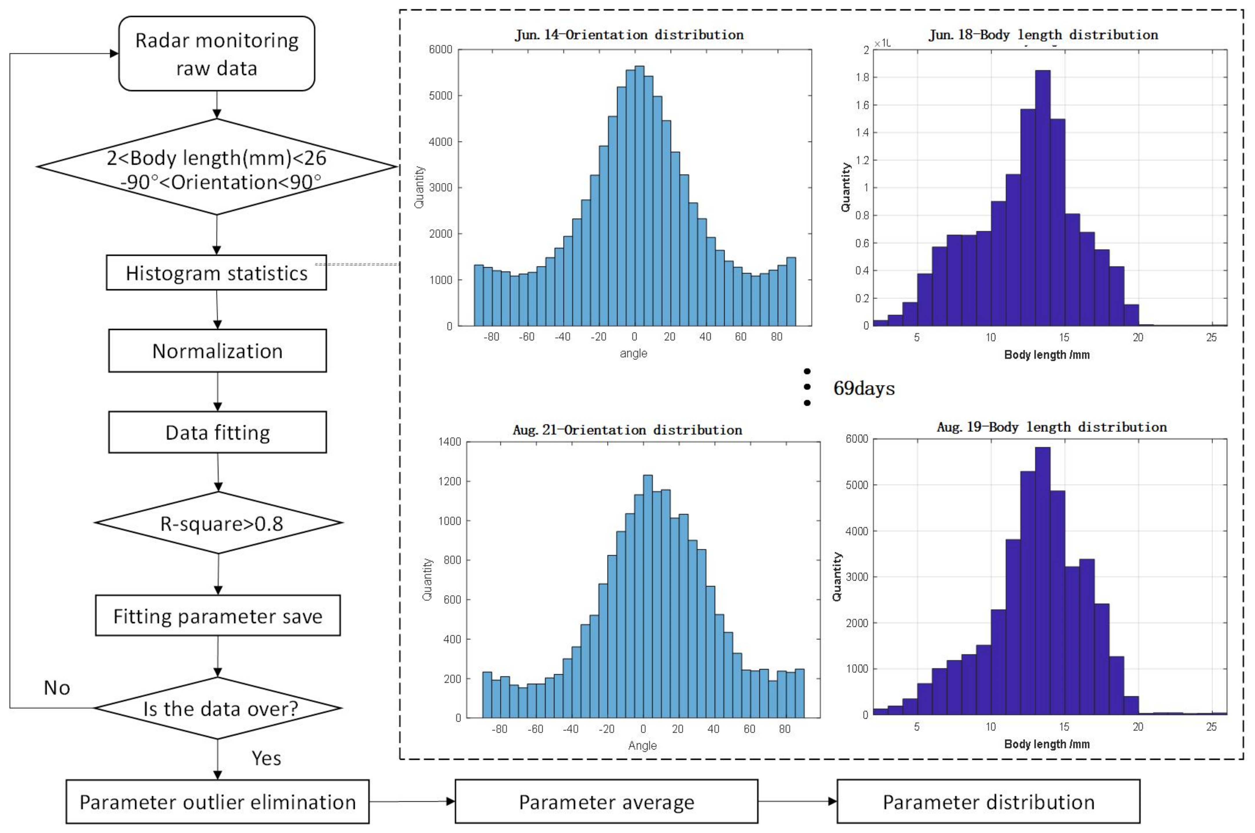
- Based on the long-term monitoring data from Ku-band fully polarimetric entomological radar, we obtained the probability distribution model for the body length and orientation of migratory insects.
- 2.
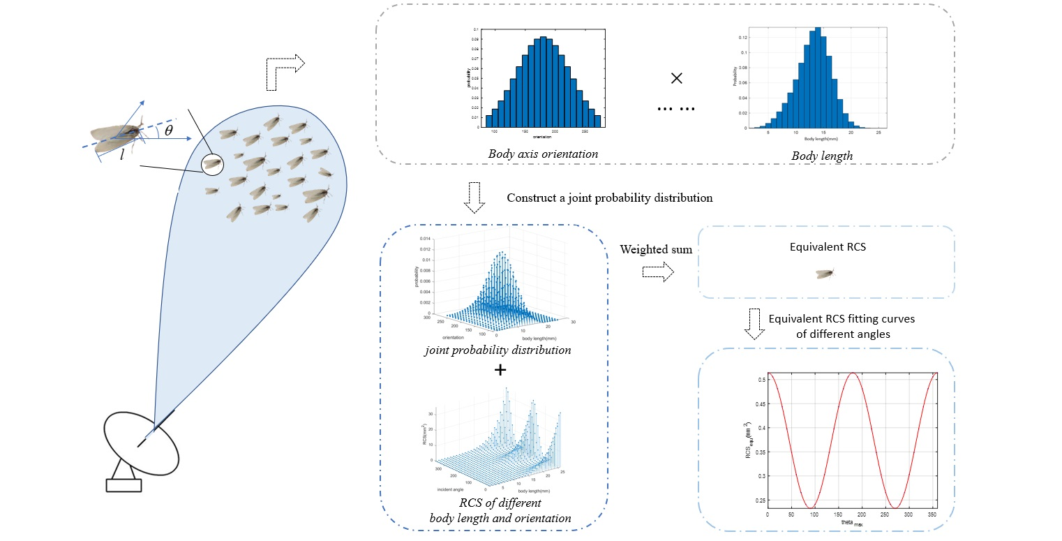
- We established an insect-equivalent RCS model, based on the joint probability distribution of “body length and incident angle”.
- 3.
- Based on the proposed model and the measured parameters of migratory insects, we simulated the RCS scattering characteristics of typical insects.
2. Materials
2.1. Entomological Radar Data
2.2. Ideal Insect RCS Simulation
3. Methods
3.1. Scattering Characteristics of Individual Insects
3.2. Retrieval Principle of Insects
3.3. Extraction of Parameters Distribution
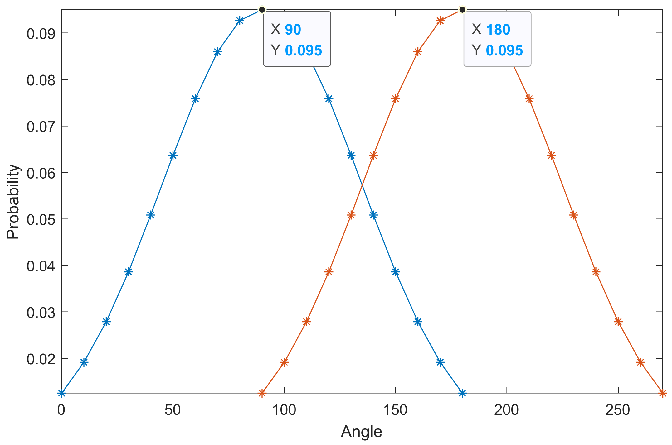
- Different from body-length distribution, the orientation of insects can vary during the migration process. Therefore, we can only find the distribution rule of insects on both sides of the orientation corresponding to the maximum distribution value (OMDV, in Equation (10)) through curve fitting, but the OMDV cannot be regarded as a fixed value. For example, Figure 6 shows the two orientation probability distribution models of OMDV at 90° and 180°. The shape factors of the two Gaussian distributions are the same, except for the fact that the OMDV is in different positions. Therefore, OMDV is a variable in the model.
- The incident angle of an individual insect is determined by the radar-transmitting wave angle and the insect orientation. When the radar-transmitting wave parameters are fixed, the change of the target incident angle is only related to the orientation. Thus, we can convert the orientation to the incident angle using Equation (11). The geometric relationship is shown in Figure 7. Then, the OMDV can be converted to the incident angle corresponding to the maximum distribution value (IAMDV).
3.4. Parametric Equivalent RCS Model
4. Results
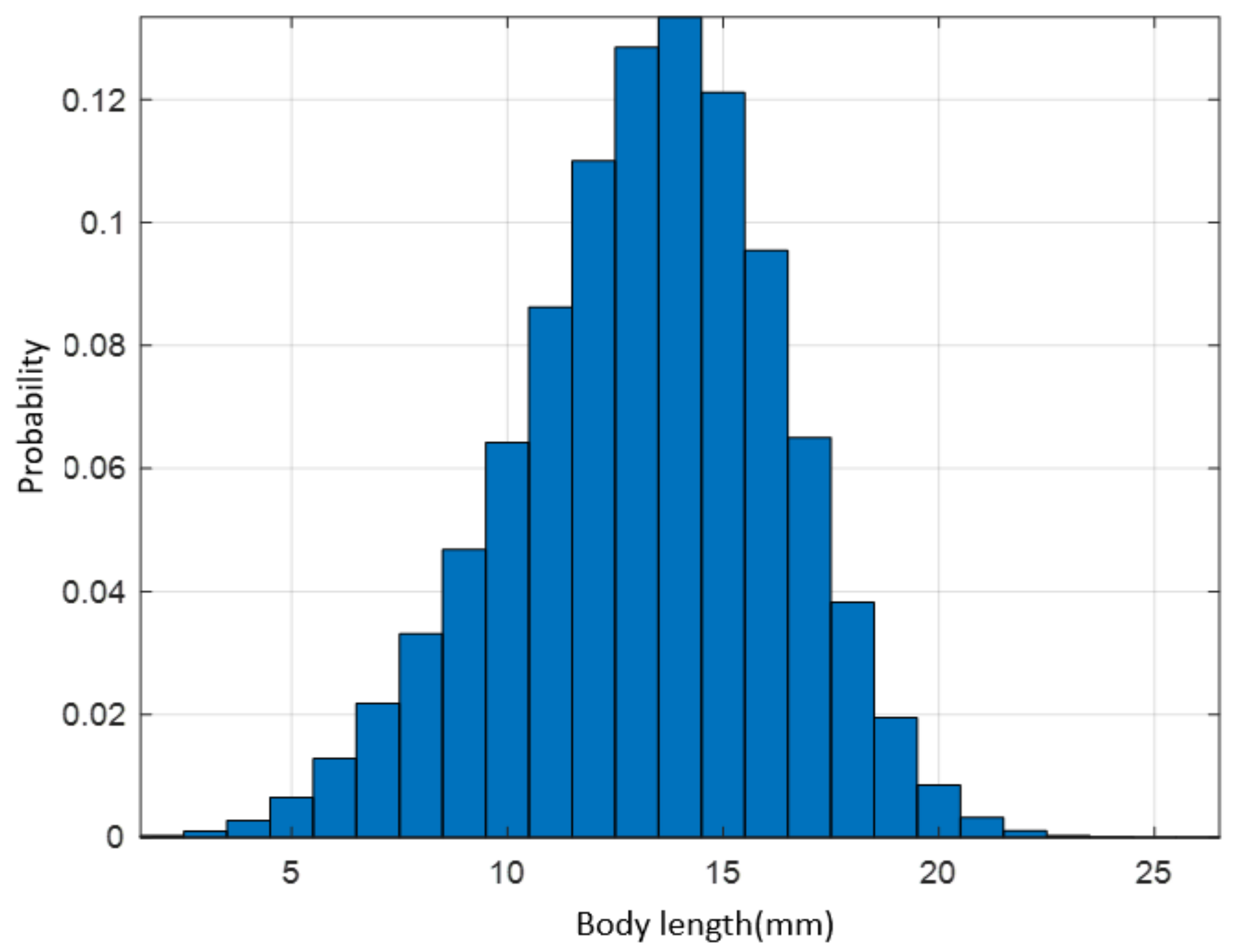
4.1. Body Length Probability Distribution Model
4.2. Incident Angle Probability Distribution Model
4.3. Simulation of Insect-Equivalent RCS Model
5. Discussion
6. Conclusions
Author Contributions
Funding
Conflicts of Interest
References
- Holland, R.A.; Wikelski, M.; Wilcove, D.S. How and why do insects migrate? Science 2006, 313, 794–796. [Google Scholar] [CrossRef] [Green Version]
- Satterfield, D.A.; Sillett, T.S.; Chapman, J.W.; Altizer, S.; Marra, P.P. Seasonal insect migrations: Massive, influential, and overlooked. Front. Ecol. Environ. 2020, 18, 335–344. [Google Scholar] [CrossRef]
- Melnikov, V.M.; Istok, M.J.; Westbrook, J.K. Asymmetric Radar Echo Patterns from Insects. J. Atmos. Ocean. Technol. 2015, 32, 659–674. [Google Scholar] [CrossRef]
- Jiang, Y.; Liu, J.; Zeng, J. Using vertical-pointing searchlight-traps to monitor population dynamics of the armyworm Mythimna separate(Walker) in China. Chin. J. Appl. Entomol. 2016, 53, 191–199. [Google Scholar]
- Bridge, E.S.; Thorup, K.; Bowlin, M.S.; Chilson, P.B.; Diehl, R.H.; Fleron, R.W.; Hartl, P.; Kays, R.; Kelly, J.F.; Robinson, W.D.; et al. Technology on the Move: Recent and Forthcoming Innovations for Tracking Migratory Birds. Bioscience 2011, 61, 689–698. [Google Scholar] [CrossRef] [Green Version]
- Wang, R.; Hu, C.; Liu, C.J.; Long, T.; Kong, S.Y.; Lang, T.J.; Gould, P.J.L.; Lim, J.; Wu, K.M. Migratory Insect Multifrequency Radar Cross Sections for Morphological Parameter Estimation. IEEE Trans. Geosci. Remote Sens. 2019, 57, 3450–3461. [Google Scholar] [CrossRef]
- Hu, C.; Li, W.D.; Wang, R.; Long, T.; Liu, C.J.; Drake, V.A. Insect Biological Parameter Estimation Based on the Invariant Target Parameters of the Scattering Matrix. IEEE Trans. Geosci. Remote Sens. 2019, 57, 6212–6225. [Google Scholar] [CrossRef]
- Gauthreaux, S.A., Jr. Weather Radar Quantification of Bird Migration. Bioscience 1970, 20, 17–19. [Google Scholar] [CrossRef]
- Cui, K.; Hu, C.; Wang, R.; Sui, Y.; Mao, H.F.; Li, H.Y. Deep-learning-based extraction of the animal migration patterns from weather radar images. Sci. China-Inf. Sci. 2020, 63, 140304. [Google Scholar] [CrossRef] [Green Version]
- Hu, C.; Cui, K.; Wang, R.; Long, T.; Ma, S.Q.; Wu, K.M. A Retrieval Method of Vertical Profiles of Reflectivity for Migratory Animals Using Weather Radar. IEEE Trans. Geosci. Remote Sens. 2020, 58, 1030–1040. [Google Scholar] [CrossRef]
- Gauthreaux, S.A.; Belser, C.G. Displays of bird movements on the WSR-88D: Patterns and quantification. Weather Forecast. 1998, 13, 453–464. [Google Scholar] [CrossRef]
- Diehl, R.H.; Larkin, R.P.; Black, J.E. Radar observations of bird migration over the Great Lakes. Auk 2003, 120, 278–290. [Google Scholar] [CrossRef]
- Chilson, P.B.; Frick, W.F.; Stepanian, P.M.; Shipley, J.R.; Kunz, T.H.; Kelly, J.F. Estimating animal densities in the aerosphere using weather radar: To Z or not to Z? Ecosphere 2012, 3, 1–19. [Google Scholar] [CrossRef]
- Hajovsky, R.; Deam, A.; LaGrone, A. Propagation, Radar reflections from insects in the lower atmosphere. IEEE Trans. Antennas Propag. 1966, 14, 224–227. [Google Scholar] [CrossRef]
- Aldhous, A.C. An Investigation of the Polarisation Dependence of Insect Radar cross Sections at Constant Aspect. Ph.D. Thesis, Cranfield University, Bedford, UK, 1989. [Google Scholar]
- Vaughn, C.R. Birds and insects as radar targets—A review. Proc. IEEE 1985, 73, 205–227. [Google Scholar] [CrossRef]
- Murton, R.K.; Wright, E.N. The Problems of Birds as Pests: Proceedings of a Symposium Held at the Royal Geographical Society, London, on 28 and 29 September 1967; Elsevier: New York, NY, USA, 2013; pp. 53–86. [Google Scholar]
- Mirkovic, D.; Stepanian, P.M.; Wainwright, C.E.; Reynolds, D.R.; Menz, M.H.M. Characterizing animal anatomy and internal composition for electromagnetic modelling in radar entomology. Remote Sens. Ecol. Conserv. 2019, 5, 169–179. [Google Scholar] [CrossRef]
- Rui, W.; Weidong, L.; Cheng, H.; Muyang, L.; Huafeng, M. Insect Biological Parameters Estimation Method and Field Quantitative Experiment Verification for Fully Polarimetric Entomological Radar. J. Signal Processing 2021, 37, 199–208. [Google Scholar] [CrossRef]
- Townes, H. A light-weight Malaise trap. Entomol. News 1972, 83, 239–247. [Google Scholar]
- Macaulay, E.D.M.; Tatchell, G.M.; Taylor, L.R. The rothamsted insect survey 12-metre suction trap. Bull. Entomol. Res. 1988, 78, 121–129. [Google Scholar] [CrossRef]
- Drake, V.A.; Reynolds, D.R. Radar Entomology: Observing Insect Flight and Migration; Cabi: Wallingford, UK, 2012. [Google Scholar]
- Hu, C.; Li, W.D.; Wang, R.; Long, T.; Drake, V.A. Discrimination of Parallel and Perpendicular Insects Based on Relative Phase of Scattering Matrix Eigenvalues. IEEE Trans. Geosci. Remote Sens. 2020, 58, 3927–3940. [Google Scholar] [CrossRef]
- Teng, Y.; Rui, W.; Muyang, L.; Cheng, H. Research on the Design and Calibration of Wideband Fully Polarized Vertical Insect Radar. J. Signal Processing 2021, 37, 222–233. [Google Scholar] [CrossRef]
- Stepanian, P.M.; Entrekin, S.A.; Wainwright, C.E.; Mirkovic, D.; Tank, J.L.; Kelly, J.F. Declines in an abundant aquatic insect, the burrowing mayfly, across major North American waterways. Proc. Natl. Acad. Sci. USA 2020, 117, 2987–2992. [Google Scholar] [CrossRef] [PubMed]
- Marshall, J. The distribution of raindrops with size. J. Atmos. Sci. 1948, 5, 165–166. [Google Scholar] [CrossRef]
- Hu, C.; Li, W.; Wang, R.; Liu, C.; Zhang, T.; Li, W. Accurate Insect Orientation Extraction Based on Polarization Scattering Matrix Estimation. IEEE Geosci. Remote Sens. Lett. 2017, 14, 1755–1759. [Google Scholar] [CrossRef]
- Muyang, L.; Rui, W.; Teng, Y.; Cheng, H. Influence of Channel Imbalance on Insect Orientation Estimation in Fully Polarimetric Radar. J. Signal Processing 2021, 37, 177–185. [Google Scholar] [CrossRef]
- Kong, S.Y.; Hu, C.; Wang, R.; Zhang, F.; Wang, L.J.; Long, T.; Wu, K.M. Insect Multifrequency Polarimetric Radar Cross Section: Experimental Results and Analysis. IEEE Trans. Geosci. Remote Sens. 2021, 59, 6573–6585. [Google Scholar] [CrossRef]
- Doviak, R.J.; Zrnic, D.S.; Sirmans, D.S. Doppler weather radar. Proc. IEEE 1979, 67, 1522–1553. [Google Scholar] [CrossRef]
- Ishimaru, A. Wave Propagation and Scattering in Random Media; Academic Press: New York, NY, USA, 1978; Volume 1, pp. 407–460. [Google Scholar]


| Parameter | Value |
|---|---|
| Frequency (GHz) | 16.2 (Ku band) |
| Waveform | Stepped-frequency chirp |
| Beamwidth | 1.5° |
| Peak power (W) | 30 |
| Synthetic bandwidth (MHz) | 800 |
| Range resolution (m) | ~0.2 |
| Antenna diameter (cm) | 12 |
| Pulse width (us) | 1 |
| IAMDV | 90° | 100° | 110° | 120° | 130° |
| Equivalent RCS (mm2) | 0.514 | 0.506 | 0.481 | 0.444 | 0.400 |
| IAMDV | 140° | 150° | 160° | 170° | 180° |
| Equivalent RCS (mm2) | 0.349 | 0.303 | 0.266 | 0.241 | 0.233 |
Publisher’s Note: MDPI stays neutral with regard to jurisdictional claims in published maps and institutional affiliations. |
© 2022 by the authors. Licensee MDPI, Basel, Switzerland. This article is an open access article distributed under the terms and conditions of the Creative Commons Attribution (CC BY) license (https://creativecommons.org/licenses/by/4.0/).
Share and Cite
Wang, R.; Kou, X.; Cui, K.; Mao, H.; Wang, S.; Sun, Z.; Li, W.; Li, Y.; Hu, C. Insect-Equivalent Radar Cross-Section Model Based on Field Experimental Results of Body Length and Orientation Extraction. Remote Sens. 2022, 14, 508. https://doi.org/10.3390/rs14030508
Wang R, Kou X, Cui K, Mao H, Wang S, Sun Z, Li W, Li Y, Hu C. Insect-Equivalent Radar Cross-Section Model Based on Field Experimental Results of Body Length and Orientation Extraction. Remote Sensing. 2022; 14(3):508. https://doi.org/10.3390/rs14030508
Chicago/Turabian StyleWang, Rui, Xiao Kou, Kai Cui, Huafeng Mao, Shuaihang Wang, Zhuoran Sun, Weidong Li, Yunlong Li, and Cheng Hu. 2022. "Insect-Equivalent Radar Cross-Section Model Based on Field Experimental Results of Body Length and Orientation Extraction" Remote Sensing 14, no. 3: 508. https://doi.org/10.3390/rs14030508
APA StyleWang, R., Kou, X., Cui, K., Mao, H., Wang, S., Sun, Z., Li, W., Li, Y., & Hu, C. (2022). Insect-Equivalent Radar Cross-Section Model Based on Field Experimental Results of Body Length and Orientation Extraction. Remote Sensing, 14(3), 508. https://doi.org/10.3390/rs14030508