DA-IMRN: Dual-Attention-Guided Interactive Multi-Scale Residual Network for Hyperspectral Image Classification

Abstract

Deep learning-based fusion of spectral-spatial information is increasingly dominant for hyperspectral image (HSI) classification. However, due to insufficient samples, current feature fusion methods often neglect joint interactions. In this paper, to further improve the classification accuracy, we propose a dual-attention-guided interactive multi-scale residual network (DA-IMRN) to explore the joint spectral-spatial information and assign pixel-wise labels for HSIs without information leakage. In DA-IMRN, two branches focusing on spatial and spectral information separately are employed for feature extraction. A bidirectional-attention mechanism is employed to guide the interactive feature learning between two branches and promote refined feature maps. In addition, we extract deep multi-scale features corresponding to multiple receptive fields from limited samples via a multi-scale spectral/spatial residual block, to improve classification performance. Experimental results on three benchmark datasets (i.e., Salinas Valley, Pavia University, and Indian Pines) support that attention-guided multi-scale feature learning can effectively explore the joint spectral-spatial information. The proposed method outperforms state-of-the-art methods with the overall accuracy of 91.26%, 93.33%, and 82.38%, and the average accuracy of 94.22%, 89.61%, and 80.35%, respectively.

1. Introduction

With the advances of imaging technology, HSIs are able to capture the full optical spectrum simultaneously for all pixels in a single acquisition. The abundant spectral information enables HSIs to distinguish different materials. There has been increasing research interest in combining machine learning and HSIs [1,2], and great progress was reported in precision agriculture, environmental monitoring, military, mineralogy, etc. In these applications, HSI classification, which aims to assign a unique label to each pixel, is a fundamental problem in HSI analysis [3,4,5]. However, due to the limited sample size and the spatial variability [6], there are remaining major challenges for HSI classification: First, the dimensionality concern is inevitable with the increase of feature size for limited samples; Second, due to changes in factors such as illumination, environment, atmosphere, and time conditions, spatial variations of spectral characteristics may signify the phenomenon of “same matter with different spectrum” and “distinct matter with similar spectrum” [7].

Both spectral and spatial information are meaningful in HSI classification, whereas early HSI classification methods primarily focused on spectral information [8,9]. Numerous feature extraction methods were proposed to extract discriminating spectral features, while ignoring the spatial relationship between adjacent pixels [10]. Traditional classifiers include random forest [11], support vector machines (SVM) and their variants [12]. However, such methods may be unsatisfying for missing the complementary spatial information. The high spatial resolution provides abundant spatial structure information of the targeted objects. Methods based on spatial features, such as gray level co-occurrence matrix (GLCM) [13] and Gabor filter [14] were exploited. Currently, the spectral-spatial analysis is the main stream for HSI classification. For instance, Kang et al. used Edge Preserving Filtering (EPF) as a post-processing technique to optimize the probability results of SVM [15]. Methods such as morphological profile [16] and composite kernels [17] also took advantage of spectral and spatial features. They generally provide improved HSI classification performance when compared with the methods based on only spectral features.

The above-mentioned HSI classification methods include two major steps: feature extraction and classification. They mainly focus on designing effective feature representations, whereas such shallow handcrafted features limited power in representing the abundant spectral-spatial information and cannot fully explore the complicated nature of HSIs. Recently, deep learning has achieved remarkable performance in various fields, such as intelligent speech [18], object detection [19], image segmentation [20] and medical image analysis [21,22]. Benefiting from their ability to extract high-level, semantic features, deep learning methods revolutionized HSI classification, and are becoming a new trend in HSI analysis. Stacked autoencoders (SAEs) and the variants were employed to extract high-level features. For instance, Chen et al. used stacked autoencoders to extract high-level features after feature dimensionality reduction [23]. Tao et al. employed a stacked sparse auto-encoder network to directly learn an incomplete sparse spectral feature representation from the original hyperspectral data, which solved the redundancy problem of high-dimensional data without any dimensionality reduction technique [24]. To extract spectral-spatial information, Ma et al. proposed an improved SAE, namely spatial updated deep autoencoder, and updated the features in consideration of the contextual information [25]. Moreover, Chen et al. also verified the eligibility of deep belief networks (DBN) in the HSI spectral-spatial analysis [26].

However, both SAE and DBN only accept one-dimensional input, and thus may overlook the spatial pattern and deteriorate the classification performance. To address this concern, Yue et al. [27] introduced the deep convolutional neural network (DCNN) into remote sensing for the first time. They used the DCNN to extract spectral and spatial features hierarchically and fine-tune the model by adding logistic regression to the classifier to improve the classification accuracy. By considering the spatial information, the CNN-based approach has become somewhat mainstream for HSI classification. However, the earlier several methods exploited the spectral and spatial information separately, neglecting the correlations between them. For instance, Wenzhi et al. employed a local discriminant embedding algorithm to extract spectral features and used a CNN-based framework to extract high-level spatial features. Such features were then fused for HSI classification [28]. Although fusion of spectral and spatial features provides performance improvement over the fully connected SAE and DBN models, there are still spectral-spatial information loss. Considering the intrinsic 3D characteristic of HSIs, it is reasonable to exploit spectral-spatial features simultaneously via 3D-CNN [1,29]. These features were demonstrated to be useful for better and robust HSI classification. For instance, Wang et al. introduced the Jeffries-Matusita distance to select effective bands and employed a 3D-CNN to mine spectral and spatial features [30]. Ma et al. proposed a two-branch network to extract these two types of features simultaneously, and then fused them for classification [31]. Furthermore, Zou et al. exploited the spectral-spatial information by the fusion of 3D-FCN and 1D-FCN, and demonstrated that the spectral information might be more powerful in analyzing HSIs with low spatial resolution [32]. Similarly, a few recent two-branch 3D-CNNs could be found in [33,34]. However, most of these methods only fused the spectral and spatial features via concatenation prior to the final classification.

Although the 3D-CNN-based methods achieved promising performance, there are remaining concerns to be addressed. First and foremost, how to learn discriminative spectral-spatial features is critical, especially for the cases with limited samples. In HSI classification, accurately labeled samples are rather limited, whereas the number of parameters in a 3D-CNN is huge. This is a serious obstacle to fully exploit the spectral-spatial information via 3D-CNN. Secondly, although a 3D-CNN extracts spectral and spatial features simultaneously, its power to learn the joint interactions between these two types of features is limited. Most existing methods for spectral-spatial learning did not realize such information interactions in feature learning. They just extracted the spectral/spatial features independently and stacked them. Thirdly, the patch-wise classification methods based on CNNs generally predict the label of a central pixel with the help of neighbour information, and then predict all the labels via the sliding window strategy. However, the reported results might be over-optimistic due to the potential training-testing information leakage [4,5]. Although the pixel-wise classification provides an effective alternative of the patch-wise classification [35], there is still much space to improve the performance without information leakage. Those methods only extract single-scale features from fixed-size image patches and cannot guarantee to capture the optimal spatial context information.

To address the above concerns, we propose a dual-attention-guided interactive multi-scale residual network to predict the label of each pixel in given HSIs. The main contributions are summarized as follows:

• We propose a dual-attention-guided interactive feature learning strategy, including the spatial and channel attention module (SCAM) as well as the spectral attention module (SAM). We interpret the problem of assigning label to each pixel as the pixel-to-pixel classification task, rather than the traditional patch-wise classification. The proposed network interactively extracts joint spectral-spatial information and performs feature fusion to enhance the classification performance. By adjusting the weights of feature maps from three different dimensions, the bidirectional attention can guide feature extraction effectively.
• We introduce a multi-scale spectral/spatial residual block (MSRB) for classification. It uses different kernel sizes at the convolutional layer to extract the features corresponding to multiple receptive fields, and provides abundant information for pixel-level classification.
• We evaluate the proposed modules and report their performance over three popular benchmark datasets. Extensive experimental results demonstrate that the proposed DA-IMRN outperforms state-of-the-art HSI classification methods. The related codes are publicly available at the following website: https://github.com/usefulbbs/DA-IMRN (accessed on 21 January 2021).

2. Methodology

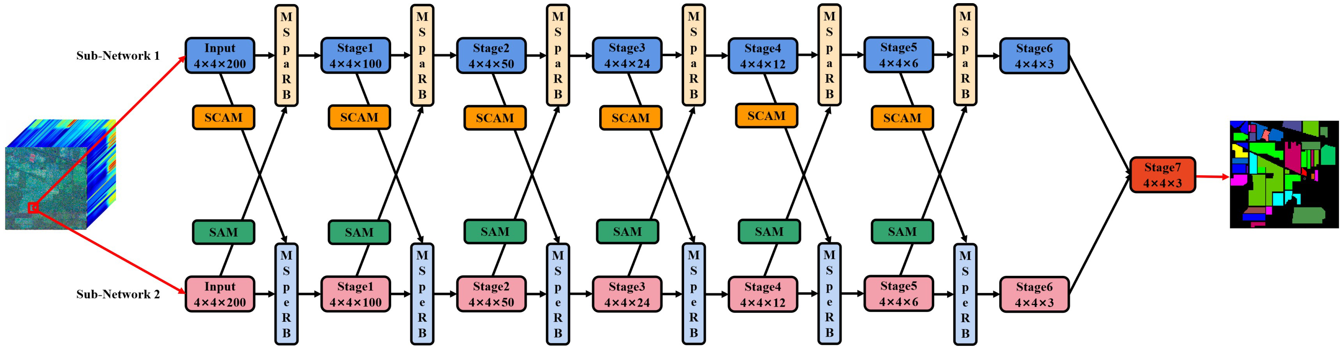
2.1. Proposed Framework

With limited samples, in order to exploit spectral-spatial interactions and extract multi-scale features, we proposed a dual-attention-guided interactive multi-scale residual network for HSI classification, as shown in Figure 1. In general, the proposed network consists of three key parts. First, two branches are used to extract the joint spectral and spatial features of HSIs, providing stronger feature extraction capabilities than the single-branch serial network. Second, inspired by the success of the multi-attention mechanism in computer vision [36], the dual-attention module, including the SCAM and SAM, is designed to adjust the weights of feature maps and exploit the joint information for improving classification performance. In contrast to traditional multi-branch networks, which mostly only use feature stacking at the end of the feature extraction stage, we employ SCAM and SAM to interactively update the feature information between two branches. Third, MSRB is constructed to extract deep multi-scale features corresponding to multiple receptive fields from limited samples.

2.2. Dual-Attention Mechanism

Inspired by the human visual attention process, various attention-based models achieved remarkable performance in semantic segmentation, pattern recognition, target detection, and other fields [37,38,39]. In RGB image segmentation tasks, spatial attention mechanism and channel attention mechanism are usually used after feature extraction to redistribute feature weights and achieve the refined segmentation results. The channel-wise attention determines the importance of feature channels and adjusts their weights in network propagation. Similarly, the spatial-wise attention is to generate a probability map for each pixel in the area to strengthen the correlation between adjacent pixels. Compared to RGB images, HSIs have a higher spectral resolution and provide abundant information of the land cover. Therefore, it is necessary to introduce the spectral-wise attention to select important bands and enhance the distinguish ability of spectral features. In this paper, we propose a dual-attention mechanism, which consists of SCAM and SAM. The dual-attention mechanism comprehensively considers the joint interactions between spatial-channel-spectral dimensions in the feature learning process and adjusts their weights dynamically.

2.2.1. Spatial-Wise & Channel-Wise Attention Module

The environmental factors such as light, temperature, and humidity have a great influence on hyperspectral imaging. Intra-class inconsistency and inter-class homogeneity greatly affect the classification performance. The way which is able to effectively explore the spatial information and the corresponding contextual dependencies is the key to solve this problem [40]. In addition, in the process of feature extraction, different channels in each convolutional stage can be regarded as different feature representations [40,41], whereas many of them are meaningless feature channels. Therefore, we need to adjust the channel weight, increasing the weight of useful channels and weakening the weight of useless channels. In this paper, we combine the channel attention with the spatial attention, and propose the SCAM, as shown in Figure 2a.

After being fed into the SCAM, the feature map will be sent to four different ramifications simultaneously, including one for channel attention and the others for spatial attention. The size of the input feature map is denoted by $P\times P\times B\times C$, where P, B, and C represents the width/height, bands, and channels of feature maps. In the channel attention ramification, the input feature map is first sent into a global average pooling (GAP) layer to aggregate spectral-spatial information into a $1\times 1\times 1\times C$ feature vector. Then, this vector passes through a fully connected (FC) layer and a ReLU activation layer to exploit the non-linearity and learn complex structures in the data. Subsequently, another FC layer is employed to adjust the dimension of the vector back to $1\times 1\times 1\times C$, and a Sigmoid activation function maps the feature vector to a probability vector, which is a channel weight of the original feature maps. In the spatial attention ramifications, we incorporat different convolution kernel sizes to downsample the original feature map in three ramifications, and obtain spatial attention feature maps of different scales. In these three ramifications, we employ convolution with only one filter to aggregate channel information, and then apply the Sigmoid activation function to generate probability maps. Ramification-spatial-one employs a convolutional layer whose kernel size and stride are both (1, 1, 1) and generates a probability map with the same size of spatial dimension as the input feature map. The difference is that the input of ramification-spatial-two first passes through a convolutional layer whose kernel size and stride are both (P/2, P/2, 1). Thus, the pixels in the $2\times 2$ region share the same weight, therefore increasing the probability that adjacent pixels belong to the same class. The kernel size and the stride of ramification-spatial-three are halved in comparing with the previous one. After the convolutional layer, the probability results of ramification-spatial-two and ramification-spatial-three are upsampled to $P\times P\times B\times 1$. In the case that the input patch-width equals to 4 or is not a multiple of 4 (for example, width/height = 6, 10…), we will discard the ramification-spatial-three. Finally, the original feature map is multiplied with the average weight obtained in the channel-wise attention and spatial-wise attention, and the product is added to the input feature map. This attention mechanism is able to regulate the weight of each value in the three-dimensional feature map, which can be expressed as:

$$W_{Cha}\left(x\right)={\sigma }_{Sigmoid}(f_{FC2}\left({\sigma }_{ReLU}\left(f_{FC1}\left(f_{GAP}\left(x\right)\right)\right)\right)$$

(1)

$$W_{Spa1}\left(x\right)={\sigma }_{Sigmoid}\left({\sigma }_{ReLU}\left(f_{Conv}\left(x\right)\right)\right)$$

(2)

$$W_{Spa2}\left(x\right)=f_{Resize}\left({\sigma }_{Sigmoid}\left({\sigma }_{ReLU}\left(f_{Conv}\left(x\right)\right)\right)\right)$$

(3)

where x is the $P\times P\times B\times C$ input feature map and $f_{GAP}$ is the global average pooling function. $f_{FC1}$ and $f_{FC2}$ is the first and the second FC layers, respectively. ${\sigma }_{ReLU}$ is the ReLU function, and ${\sigma }_{Sigmoid}$ is the Sigmoid activation layer. $f_{Conv}$ is the convolution function, $f_{Resize}$ denotes upsampling.

The final output of SCAM can be computed as:

$$F_{SCAM}\left(x\right)=x+x*Average(W_{Cha}\left(x\right),W_{spa1}\left(x\right),W_{spa2}\left(x\right))$$

(4)

where x is the $P\times P\times B\times C$ input feature map.

2.2.2. Spectral-Wise Attention Module

As to the spectral-dimension, it can be expressed as a continuous spectral curve containing each spectral value. Mostly, hundreds of spectral bands are directly used as input of the convolutional layer, whereas the noisy bands among them might deteriorate the classification performance. Therefore, we propose a spectral attention module that enables the network to recalibrate the importance of different spectral bands and enhance useful spectral features, as shown in Figure 2b. The input feature with the size of $P\times P\times B\times C$ is sent to the convolutional layer and the ReLU layer, and only one filter is used to fuse information from different channels. The kernel size and stride of the convolutional layer are set to (P, P, 1) without padding. This operation combines the spatial information and produces a vector of $1\times 1\times B\times 1$. Subsequently, the output of the convolutional layer is sent to the Sigmoid function to obtain the probability vector. For convenience, the probability vector is upsampled to the size of the input feature map. The weighted feature map is obtained by multiplying the input feature with the probability map. Then, the product is added to the input feature map, and the result is the output of the SAM module. Mathematically, the SAM can be expressed as:

$$F_{SAM}\left(x\right)=x+x\ast f_{Resize}\left({\sigma }_{Sigmoid}\left({\sigma }_{ReLU}\left(f_{Conv}\left(x\right)\right)\right)\right)$$

(5)

where x is the $P\times P\times B\times C$ input feature, $f_{Conv}$ is the convolution function, $f_{Resize}$ denotes upsampling, ${\sigma }_{ReLU}$ is the ReLU function, and ${\sigma }_{Sigmoid}$ is the Sigmoid activation layer.

2.3. Multi-Scale Residual Block (MSRB)

To avoid potential information leakage, the authors of [32,35] interpreted the problem of HSI classification as an semantic segmentation problem, which is able to fully use the limited annotations. To further improve the performance, especially on small HSIs, we introduce the multi-scale residual network to deepen the network and extract multi-scale spectral/spatial features.

2.3.1. Residual Learning

Compared with shallow networks, deep networks demonstrated stronger learning capabilities and feature expression capabilities, and are able to learn more abstract features [42,43]. However, if the network becomes too deep with too many parameters, it will require huge amount of data to be well tuned. Otherwise, it will most probably perform well on the training set but poorly on the test set (degradation problem). To address this concern, He et al. [43] proposed residual learning, as shown in Figure 3, where $f_{Res}\left(x\right)$ represents a residual function. In the forward propagation process, after the shallow layer completes feature extraction, residual learning enables the deep network to implement identity mapping. Therefore, it can propagate gradients directly to initial layers and trains deeper networks. In particular, He et al. pointed out that the shortcut connection is more economical and practical than the non-shortcut connection with dimension adjustment [43]. A few recent residual-network-based methods for HSI classification which achieved significant performance improvement can be found in [44,45].

2.3.2. Multi-Scale Spectral/Spatial Residual Block

Although the recent HSI classification methods based on deep learning achieved remarkable performance, most of them only considered the features under single scale. Previous studies demonstrated the effectiveness of multi-scale features in HSI classification [46,47]. To extract spectral/spatial features at different scales, we introduce a novel multi-scale spectral/spatial module into a residual block, and employ the combination in solving classification problems. The MSRB is realized by replacing the convolutional layers with a branch structure containing three convolution kernels with different sizes. As shown in Figure 4, unlike the conventional residual unit, we employ a $1\times 1\times 1$ convolutional layer and a batch normalization layer as the first component of the MSRB to unify the number of channels, downsample spectral bands, and combine information. Then, a multi-scale residual convolution group is applied to improve feature extraction. These multi-scale residual convolution groups with three convolution kernels of different sizes are used to construct feature representations of different scales. Furthermore, we employ the concatenate operation to merge the output feature maps corresponding to three scales and obtain the fused feature. Then the feature maps are passed to $1\times 1\times 1$ convolutional layer to obtain consistent dimension.

The detailed structure of the proposed multi-scale spectral residual block (MSpeRB) and multi-scale spatial residual block (MSpaRB) is shown in Figure 4a and Figure 4b, respectively. The main difference between these two blocks is the sizes of the convolution kernels in the multi-scale learning stages. As to the MSpeRB, we select the kernel size as $1\times 1\times m$ ($m_1$ = 3, $m_2$ = 5, $m_3$ = 7). As to the MSpaRB, the corresponding kernels are with the sizes of $m\times m\times 1$ ($m_1$ = 3, $m_2$ = 5, $m_3$ = 7). With the aid of these two blocks, the network is able to capture different levels of spectral/spatial features corresponding to multiple receptive fields in each channel, and therefore obtain more abundant information to enhance the classification performance.

3. Experiment Result and Analysis

In this section, we evaluate the effectiveness of the proposed DA-IMRN on three benchmark datasets, including Salinas Valley (SV), Pavia University (PU) and Indian Pines (IP). We compare the proposed method with five state-of-the-art HSIs classification algorithms without information leakage. In addition, we refer the interested readers to [4,5] for further details and discussions about the potential information leakage from the overlap between training set and testing set in traditional patch-wise HSI classification.

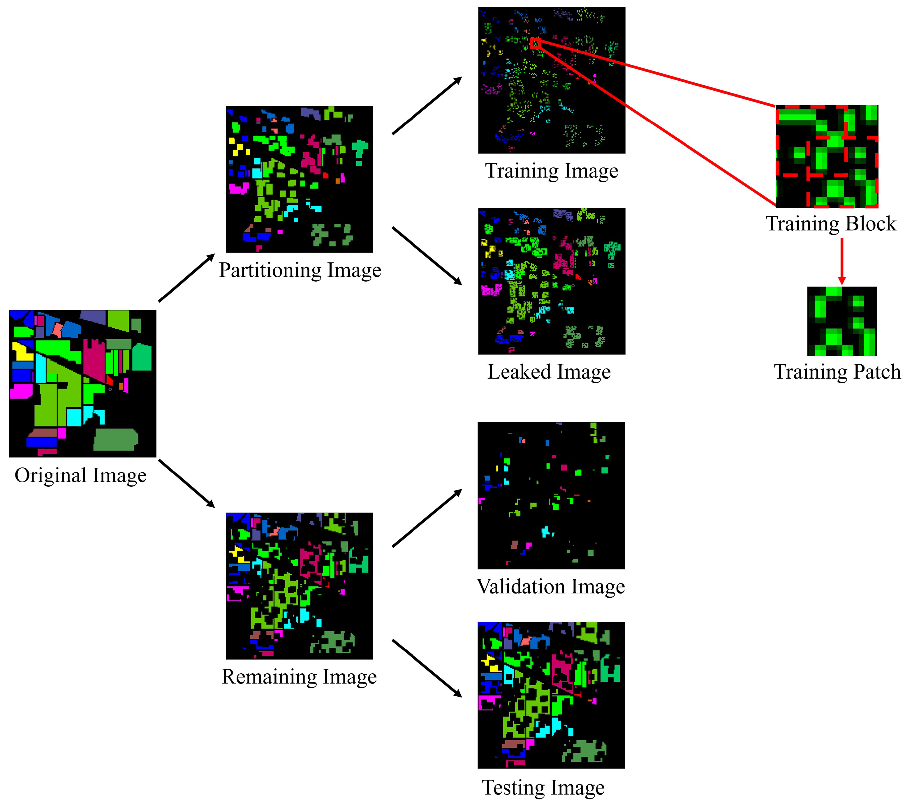
3.1. Dataset Partition

Nalepa et al. showed in [4] that the traditional patch-based classification methods in tandem with the corresponding data partitioning strategies, which aim to predict the label of the central pixel, might lead to potential information leakage. In HSI classification, the division of training/testing sets greatly affects the performance and fairness of the comparison. Therefore, a dataset partitioning strategy, which enables fair validation of new and existing algorithms without training-testing data leakage, is highly desired. Several data partitioning methods that will not lead to information leakage were proposed [4,32,35]. Among them, the dataset partition in [35] not only provides a benchmark dataset, but also avoids the loss of samples of certain classes in the training/testing sets. It divides the original image into training/validation/testing blocks and then subdivides the training/validation/testing sets, making the division method more reasonable and more suitable for practical applications. In this work, we apply the same data partition strategy as in [35] to avoid information leakage. Specifically, as show in Figure 5, we apply the same sliding window strategy in [32] to training blocks and testing blocks (which are divided from the original images) to obtain more training/validation/testing patches. Then we continue to expand our training and testing patches by using classical data enhancement methods (flip up/down, flip right/left, rotate with an angle of $\pi$ or $\pi /2$). We only use two of these three augmentation methods for each patch to guarantee the randomness of the expanded data.

3.2. Dataset Description

In the experiments, in order to reduce the influence of randomness, we employ hold-out test and repeat for 25 times to obtain the average performance. Each round of hold-out test is independent of the other ones, and the training pixels for 5-round of them are shown in Figure 6, including (a1–a5), (b1–b5) and (c1–c5) corresponding to three datasets. The details of three datasets and related settings are as follows:

(1) Salinas Valley: This dataset was captured by the AVIRIS sensor in Salinas Valley of California USA with a resolution of 3.7 m/pixel. It is composed of $512\times 217$ pixels, 204 bands after discarding 20 water absorption bands. This dataset contains 16 classes of ground truth, shown in Figure 6(a0). In total, there are 2017.2 pixels used for training on average, accounting for 3.73% of all the labeled pixels.

(2) Pavia University: This dataset was obtained by the ROSIS sensor over the University of Pavia with a high resolution of 1.3 m/pixel. It is composed of $610\times 340$ pixels and 103 spectral bands after discarding 12 noisy bands. This dataset consists of 9 classes of ground truth, shown in Figure 6(b0). 6.31% of the labeled pixels (around 2701.4 pixels) are used for training.

(3) Indian Pines: This dataset was captured by the AVIRIS sensor over Indian Pines region in North-western Indian in 1992. It contains $145\times 145$ pixels and 204 spectral bands after removing 20 water absorption bands. It contains 16 classes of ground truth. The ground truth, shown in Figure 6(c0). There are about 1187.8 pixels on average are used for training, accounting for 11.59%.

3.3. Evaluation Matrices

To evaluate the robustness and effectiveness of the proposed method, the overall accuracy (OA), average accuracy (AA), and Kappa coefficient are employed in this study. Specifically, the OA metric refers to the ratio of the total number of the correctly classified pixels over all test pixels [48]. The AA metric is the average classification accuracy of all classes [48]. The Kappa coefficient measures the degree of agreement between the predictions and the ground-truth [48]. These three evaluation matrices collectively reflect the performance of HSI classification, and the higher value represents the better performance. Let $\mathit{M}\in {\mathbb{R}}^{n\times n}$ represents the confusion matrix of the classification results, n denotes the number of land cover categories and the value of $\mathit{M}$ in $\left(\mathit{i},\mathit{j}\right)$ position indicates the number of $\mathit{i}$th category samples that are classified to the $\mathit{j}$th category. The three evaluation metrics can be expressed as:

$$\mathit{OA}=\mathit{sum}\left(\mathit{diag}\right(\mathit{M}\left)\right)./\mathit{sum}\left(\mathit{M}\right))$$

(6)

$$AA=mean\left(diag\right(M)./sum(M,2\left)\right)$$

(7)

$$kappa=\frac{OA-\left(sum(M,1)sum(M,2)\right)/sum{\left(M\right)}^2}{1-\left(sum(M,1)sum(M,2)\right)/sum{\left(M\right)}^2}$$

(8)

where $diag\left(M\right)\in {\mathbb{R}}^{n\times 1}$ is a vector of diagonal elements of M, $sum(·)\in {\mathbb{R}}^1$ is the sum of all elements, $sum(·,1)\in {\mathbb{R}}^{1\times n}$ is the vector of the sum of elements in each column, $sum(·,2)\in {\mathbb{R}}^{n\times 1}$ is the vector of the sum of elements in each row, $mean(·)\in {\mathbb{R}}^1$ is the mean of all elements, and $./$ represents the element-wise division.

3.4. Parameter Setting and Network Configuration

Given the network architecture, the model performance depends on two important hyperparameters, including the block-patch size in dividing different datasets and the learning rate. We select the block size as $10\times 10$, and the patch size as $8\times 8$ for the SV & PU dataset, to ensure the balance between the number of samples and the maximum receptive field, and avoid the increase of computational cost due to a larger patch. This setting also enables generating enough training patches via the sliding window operation. Considering the spatial size of IP dataset is relatively small, we set the block size as $6\times 6$, and patch size as $4\times 4$.

Regarding to the learning rate, it controls the speed of the gradient descent during the training process, and the proper value facilitates the loss function to converge at an appropriate speed. In this work, we employ the grid search method to determine the best learning rate in 0.01, 0.005, 0.001, 0.0005 and 0.0001. The experimental results demonstrate that the optimal learning rate is 0.001 over all three datasets. In addition, we employ the learning rate decay strategy in the training process, and the learning rate is reduced to 1/10 of the previous value after every 15 epochs.

As to the network structure, most of the hyperparameters are same in terms of the kernel size and the number of filters across three datasets. The difference exists in the network for IP dataset due to its small block-patch size. We only keep two different scales with $m_1$ = 1, $m_2$ = 3 in multi-scale spatial residual block for IP dataset, and other settings are consistent across three datasets. The DA-IMRN is composed of two branch networks, and each branch network is divided into six stages. The successive two stages are connected by MSRB to extract multi-scale spectral-spatial features corresponding to multiple receptive fields. Taking the network for SV dataset as an example, the detailed kernel size of the MSRB and the output size of the feature maps in each stage are shown in

Table 1. Kernel size and feature size information in the networks (taking the SV dataset as an example).

Stage		Input	Stage1	Stage2	Stage3
Sub-Network1:		$1\times 1\times 3$	$1\times 1\times 3$	$1\times 1\times 3$	$1\times 1\times 3$
	Kernel Size	$1\times 1\times 5$	$1\times 1\times 5$	$1\times 1\times 5$	$1\times 1\times 5$
		$1\times 1\times 7$	$1\times 1\times 7$	$1\times 1\times 7$	$1\times 1\times 7$
	Feature Size	$8\times 8\times 204\times 1$	$8\times 8\times 100\times 64$	$8\times 8\times 50\times 64$	$8\times 8\times 24\times 128$
Sub-Network2:		$3\times 3\times 1$	$3\times 3\times 1$	$3\times 3\times 1$	$3\times 3\times 1$
	Kernel Size	$5\times 5\times 1$	$5\times 5\times 1$	$5\times 5\times 1$	$5\times 5\times 1$
		$7\times 7\times 1$	$7\times 7\times 1$	$7\times 7\times 1$	$7\times 7\times 1$
	Feature Size	$8\times 8\times 204\times 1$	$8\times 8\times 100\times 64$	$8\times 8\times 50\times 64$	$8\times 8\times 24\times 128$
Stage		Stage4	Stage5	Stage6	Stage7
Sub-Network1:		$1\times 1\times 3$	$1\times 1\times 3$	/	/
	Kernel Size	$1\times 1\times 5$	$1\times 1\times 5$	/	/
		$1\times 1\times 7$	$1\times 1\times 7$	/	/
	Feature Size	$8\times 8\times 12\times 128$	$8\times 8\times 6\times 256$	$8\times 8\times 3\times 256$	$8\times 8\times 3\times 256$
Sub-Network2:		$3\times 3\times 1$	$3\times 3\times 1$	/	/
	Kernel Size	$5\times 5\times 1$	$5\times 5\times 1$	/	/
		$7\times 7\times 1$	$7\times 7\times 1$	/	/
	Feature Size	$8\times 8\times 12\times 128$	$8\times 8\times 6\times 256$	$8\times 8\times 3\times 256$	$8\times 8\times 3\times 256$

. In addition, either branch interact with the other one through the dual-attention mechanism, including the SCAM and SAM. The spatial, channel and spectral information are re-weighted through the attention-guided feature learning.

The DA-IMRN is implemented in Python 3.6, Keras 2.3.1 and Tensorflow 1.14.0. To effectively improve memory use, the batch size was set to 16. We use focal loss as the loss function, designed to solve the class imbalance problem [49]. In addition, the loss function is optimized using the Nadam with beta_1 as 0.9, beta_2 as 0.999, and epsilon as $1\times {10}^{-8}$. All the experiments were performed with the same configuration on the platform with Intel i7-6850K, 64GB RAM and NVIDIA GeForce GTX 1080ti GPU.

4. Experimental Result

We compare the performance of DA-IMRN with several state-of-the-art CNN-based methods which adopt suitable data partition strategies without information leakage. The backbone structure and the ratio of pixels used for training over SV/PU/IP datasets are summarized in

Table 2. The backbone structures and the dataset partitioning of state-of-the-art HSI classification methods.

	Backbone Structure	Pixels for Training over SV/PU/IP Datasets (%)
VHIS	1D-CNN	8.91%/6.31%/19.00%
DA-VHIS	1D-CNN + Data augmentation methods	8.91%/6.31%/19.00%
AutoCNN	1D-AutoCNN	5.91%/4.20%/25.20%
SS3FCN	1D-FCN + 3D-FCN	3.76%/6.64%/11.02%
TAP-Net	Parallel network + Triple-attention mechanism	3.73%/6.36%/11.59%
DA-IMRN	Multi-scale residual network + Interactive attention-guided feature learning	3.73%/6.31%/11.59%

. In addition, in order to intuitively reflect the role of the modules we designed, we evaluate the performance of the two sub-networks of DA-IMRN.

VHIS [4]: To the best of our knowledge, ref. [4] was the first paper discussing the potential information leakage in the patch-wise classification. The authors proposed a new routine for generating classification benchmarks, and constructed a 1D-CNN-based network to extract spectral features and classify pixels without information leakage.

DA-VHIS [5]: Three data augmentation methods were proposed on the basis of [4] to improve generalization capabilities. We report the best performance of these three data augmentation methods in the comparison.

AutoCNN [50]: 1D AutoCNN was applied to optimize the classifier, and the problem of information leakage was also avoided. In addition, the authors introduced the simple but effective regularization strategy, namely cutout, to further enhance the HSI classification performance.

SS3FCN [32]: The authors interpreted the problem of assigning labels to all pixels as a semantic segmentation problem, where all label information was fully exploited. They employed a 3D fully convolutional network to jointly explore the spectral-spatial information, and introduced the other branch based on a 1D fully convolutional network to focus on spectral information. Then they fused these two branches to make the predictions via concatenation. In addition, the authors introduced a data partition strategy without information leakage.

TAP-Net [35]: A hyperspectral image classification network based on triple-attention mechanism and parallel network was designed in this work. They applied a triple-attention mechanism, including channel-wise, spectral-wise and spatial-wise attention to obtain stronger spectral-spatial representations. In addition, they introduced a more balanced dataset division strategy, which can effectively avoid information leakage and the class imbalance issue.

DA-IMRN (sub-net1): As was shown in Figure 7a, it is a serial network with the same number of stages as in the proposed DA-IMRN. The MSpaRB is employed for feature extraction. In addition, the corresponding parameter setting and network configuration are the same as DA-IMRN.

DA-IMRN (sub-net2): As shown in Figure 7b, similar to DA-IMRN (sub-net1), there are six stages within the serial network. The MSpeRB is applied for extracting features. The corresponding parameter setting as well as network configuration remain unchanged.

4.1. Classification Result on Salinas Valley

We first conduct a comparative study on the SV dataset. The average classification results of five independent repetitions over the SV dataset are shown in

Table 3. Salinas Valley dataset: Classification results in terms of per-class accuracy, OA, AA (in %), and the Kappa scores. In the last four columns, the results are displayed in the form of mean ± standard deviation.

Class	Method
	VHIS	DA-VHIS	AutoCNN	SS3FCN	TAP-Net	DA-IMRN (sub-net1)	DA-IMRN (sub-net2)	DA-IMRN
C1	85.91	96.36	96.75	92.36	$98.73\pm 1.03$	$96.90\pm 2.08$	$99.23\pm 0.52$	$98.44\pm 1.65$
C2	73.88	94.71	99.26	92.58	$99.71\pm 0.34$	$95.68\pm 5.07$	$99.67\pm 0.26$	$98.37\pm 2.58$
C3	33.72	49.95	79.46	66.35	$91.29\pm 7.74$	$85.31\pm 12.45$	$96.55\pm 2.06$	$97.75\pm 2.28$
C4	65.92	79.62	99.09	98.13	$98.78\pm 0.58$	$96.00\pm 1.71$	$98.64\pm 0.69$	$97.22\pm 1.64$
C5	46.42	64.30	97.21	95.63	$96.27\pm 2.22$	$92.45\pm 6.91$	$97.37\pm 1.53$	$92.34\pm 3.87$
C6	79.63	79.89	99.68	99.30	$99.26\pm 0.59$	$99.24\pm 0.76$	$99.59\pm 0.16$	$99.34\pm 0.38$
C7	73.59	79.62	99.35	99.43	$99.35\pm 0.32$	$99.23\pm 0.43$	$99.29\pm 0.32$	$99.05\pm 0.51$
C8	72.16	74.54	75.82	69.72	$84.76\pm 3.62$	$86.33\pm 8.34$	$83.84\pm 2.08$	$87.27\pm 4.59$
C9	71.87	96.10	99.05	99.67	$98.13\pm 1.23$	$99.07\pm 0.77$	$98.75\pm 0.68$	$99.38\pm 0.43$
C10	73.11	87.28	87.54	84.07	$88.56\pm 4.41$	$87.33\pm 4.52$	$92.04\pm 2.16$	$89.14\pm 4.62$
C11	72.51	73.08	89.15	85.31	$84.59\pm 8.04$	$94.43\pm 1.82$	$94.39\pm 3.50$	$93.82\pm 3.25$
C12	71.06	98.25	96.99	97.98	$99.02\pm 1.48$	$97.50\pm 1.08$	$99.38\pm 0.44$	$97.28\pm 2.11$
C13	75.80	97.67	98.36	98.45	$98.07\pm 1.93$	$97.21\pm 3.12$	$97.27\pm 2.97$	$97.60\pm 2.09$
C14	72.04	88.07	90.61	87.32	$94.59\pm 5.59$	$94.51\pm 7.21$	$93.69\pm 9.64$	$95.12\pm 8.28$
C15	45.03	62.92	63.47	52.31	$69.09\pm 8.00$	$62.74\pm 9.62$	$60.57\pm 2.30$	$68.86\pm 10.81$
C16	22.54	45.39	89.26	59.97	$90.71\pm 6.87$	$88.22\pm 4.88$	$92.48\pm 5.65$	$92.55\pm 4.41$
OA	64.20	77.52	87.15	81.32	$90.31\pm 1.27$	$89.12\pm 1.75$	$89.84\pm 1.02$	91.26 ± 0.89
AA	64.70	79.24	91.32	86.13	$93.18\pm 1.27$	$92.01\pm 0.64$	$93.92\pm 1.26$	94.22 ± 0.90
Kappa	/	0.749	0.857	/	$0.881\pm 0.03$	$0.879\pm 0.02$	$0.883\pm 0.01$	0.885 ± 0.03

. It can be seen from the table that the proposed DA-IMRN achieved the state-of-the-art performance compared with recent HSI classification methods. From Table 2, we known that the ratio and number of training pixels used by DA-IMRN are same as those of TAP-Net, and are less than those of VHIS, DA-VHIS, SS3FCN and AutoCNN. The OA is significantly improved via exploring multi-scale spectral-spatial joint information, in comparing with traditional spectral-based classification methods. For instance, the OA of VHIS is 64.20%, whereas the OA of the proposed DA-IMRN over five experiments is 91.26%. Although the SS3FCN and TAP-Net employed the 3D kernels to extract the joint spectral-spatial information, the representation power is still limited. Compared with these two networks, the OA & AA of DA-IMRN increases from 81.32% & 86.13%, 90.31% & 93.18% to 91.26% & 94.22%. In addition, DA-IMRN achieves the highest Kappa.

Regarding to the single branch of DA-IMRN, the OA of DA-IMRN (sub-net1) and DA-IMRN (sub-net2) are only slightly lower than TAP-Net, whereas significantly higher than SS3FCN and traditional classification methods. The AA of the DA-IMRN (sub-net2) even surpasses TAP-Net. Compared with these two separate sub-networks DA-IMRN (sub-net1) and DA-IMRN (sub-net2), DA-IMRN employs the dual-attention mechanism to guide the feature learning and realizes information interaction between two branches. The OA & AA & Kappa of DA-IMRN increased accordingly by 2.14% & 2.21% & 0.6% and 1.42% & 0.3% & 0.2%. The proposed framework is more robust even with less number of training samples. Figure 8 shows classification maps by SS3FCN, TAP-Net, DA-IMRN (sub-net1), DA-IMRN (sub-net2) and the DA-IMRN. The results of other methods are not described here due to insufficient details to reproduce the classification maps. As we can see, the classification results of the SS3FCN are not satisfactory. Especially for the upper left corner, most of the Grapes_untrained (C8) are misclassified into Vinyard_untrained (C15). Although there are a few noisy points, the results of DA-IMRN are much better than that of other counterparts.

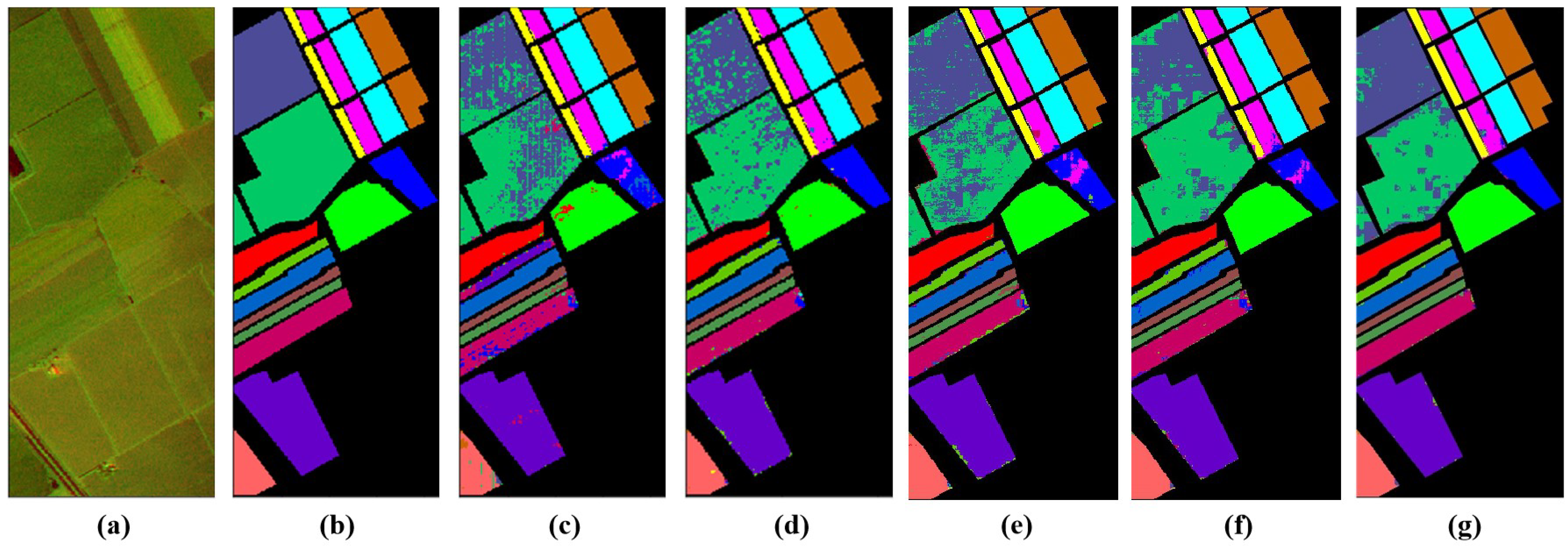
4.2. Classification Result on Pavia University

The OA, AA, Kappa and class-specific accuracy obtained by different methods over the PU dataset are shown in

Table 4. Pavia University dataset: Classification results in terms of the per-class accuracy, OA, AA (in %), and the Kappa scores. In the last four columns, the results are displayed in the form of mean ± standard deviation.

Class	Method
	VHIS	DA-VHIS	AutoCNN	SS3FCN	TAP-Net	DA-IMRN (sub-net1)	DA-IMRN (sub-net2)	DA-IMRN
C1	93.40	93.42	83.40	97.48	$95.67\pm 1.43$	$95.16\pm 4.33$	$94.16\pm 1.08$	$95.16\pm 2.58$
C2	86.20	86.52	93.32	90.86	$97.61\pm 1.39$	$98.77\pm 0.55$	$95.53\pm 1.47$	$98.43\pm 1.15$
C3	47.58	46.88	61.52	58.75	$73.08\pm 11.00$	$73.27\pm 9.83$	$87.51\pm 4.36$	$77.94\pm 11.83$
C4	86.89	92.21	78.86	84.81	$94.23\pm 1.38$	$93.14\pm 1.27$	$83.23\pm 3.07$	$94.45\pm 2.17$
C5	59.81	59.74	98.25	94.82	$99.48\pm 0.35$	$98.56\pm 1.66$	$99.43\pm 0.27$	$99.06\pm 1.57$
C6	27.14	27.68	73.34	23.59	$84.17\pm 10.26$	$87.98\pm 11.17$	$84.42\pm 10.92$	$93.99\pm 5.61$
C7	0	0	64.56	61.61	$59.92\pm 12.76$	$71.06\pm 9.32$	$46.73\pm 20.72$	$65.82\pm 11.98$
C8	78.46	78.32	76.86	88.84	$83.60\pm 7.42$	$82.02\pm 6.72$	$58.67\pm 10.24$	$83.43\pm 8.03$
C9	79.27	79.60	97.69	88.68	$99.33\pm 0.44$	$98.59\pm 1.03$	$99.09\pm 0.55$	$98.22\pm 2.22$
OA	73.26	73.84	84.63	79.89	$91.64\pm 1.08$	$92.42\pm 0.68$	$87.20\pm 1.17$	93.33 ± 1.00
AA	62.08	62.71	80.87	76.60	$87.45\pm 3.09$	$88.73\pm 1.34$	$83.20\pm 2.60$	89.61 ± 1.12
Kappa	/	0.631	0.800	/	$0.892\pm 0.02$	$0.905\pm 0.01$	$0.834\pm 0.01$	0.923 ± 0.02

. Similar to the results over the SV dataset, the proposed DA-IMRN is significantly better than VHIS, DA-VHIS, AutoCNN, SS3FCN and TAP-Net, with an average OA of 93.33%, AA of 89.61% and Kappa of 0.923. As we can see, VHIS and its variant DA-VHIS, fail to predict C7 in the testing set. The main reason is that no pixels of C7 was selected in the training process. In this work, more balanced data partitioning contributes the improvement of prediction accuracy. The accuracy of DA-IMRN over C6 increased from 84.17% of TAP-Net to 93.99%, owing to the exploration of the multi-scale joint information. In addition, different from the results over SV dataset and IP dataset, the performance of DA-IMRN (sub-net2) is worse than that of (sub-net1). This can be ascribed to the lack of spectral information for the PU dataset, which only owns 103 spectral bands. The detailed classification maps corresponding to one of five-time experiments are shown in Figure 9. Similar to the results on SV dataset, the noise is obvious in the classification result of SS3FCN. The major reason is that SS3FCN only adopted fixed kernel size, and neglected the information from multiple receptive fields. In addition, it should be noticed that the AutoCNN [50] only used 4.20% of the labeled pixels for training. To make a fair comparison, we also evaluate the performance when same number of labeled pixels are used for training. As shown in the Supplementary Table S1, the proposed DA-IMRN outperforms AutoCNN in terms of OA, AA and Kappa.

4.3. Classification Result on Indian Pines

As to the IP dataset, the spatial size is relatively small, with $145\times 145$ pixels. Therefore, we set the patch size as $4\times 4$, and only keep two different convolution kernels in the multi-scale residual blocks. The comparison results over this dataset are shown in

Table 5. Indian Pines dataset: Classification results in terms of the per-class accuracy, OA, AA (in %), and the Kappa scores. In the last four columns, the results are displayed in the form of mean ± standard deviation.

Class	Method
	VHIS	DA-VHIS	AutoCNN	SS3FCN	TAP-Net	DA-IMRN (sub-net1)	DA-IMRN (sub-net2)	DA-IMRN
C1	17.68	15.89	19.58	40.4	$70.98\pm 22.75$	$32.25\pm 37.37$	$62.75\pm 16.41$	$73.71\pm 12.19$
C2	56.89	70.41	60.16	77.89	$76.54\pm 5.92$	$71.66\pm 6.32$	$75.31\pm 8.93$	$73.72\pm 7.70$
C3	51.55	61.44	44.12	60.74	$75.62\pm 7.62$	$71.20\pm 8.44$	$72.06\pm 13.42$	$79.09\pm 5.94$
C4	36.27	42.28	25.35	11.8	$46.83\pm 17.89$	$43.84\pm 21.96$	$49.39\pm 21.80$	$62.59\pm 13.84$
C5	69.02	73.02	77.80	67.5	$69.78\pm 14.82$	$68.70\pm 19.25$	$76.90\pm 10.40$	$70.97\pm 15.39$
C6	92.35	92.13	90.99	91.95	$94.77\pm 3.96$	$91.21\pm 4.53$	$93.27\pm 2.61$	$94.36\pm 3.67$
C7	0	0	35.63	20.14	$80.40\pm 27.43$	$69.18\pm 18.42$	$50.18\pm 32.68$	$63.70\pm 17.72$
C8	86.95	86.44	95.87	81.71	$98.95\pm 1.58$	$95.33\pm 5.86$	$97.34\pm 3.05$	$97.94\pm 1.83$
C9	19.55	21.28	5.31	31.67	$70.03\pm 23.60$	$77.06\pm 8.98$	$52.85\pm 25.61$	$78.85\pm 7.95$
C10	60.05	67.47	55.93	78.15	$84.59\pm 5.99$	$84.75\pm 5.71$	$83.62\pm 2.16$	$83.87\pm 8.35$
C11	74.05	65.24	68.73	69.32	$80.39\pm 4.36$	$76.82\pm 7.24$	$77.46\pm 2.92$	$79.72\pm 4.02$
C12	43.71	49.56	36.96	40.81	$76.84\pm 6.18$	$75.84\pm 7.14$	$79.31\pm 8.15$	$79.28\pm 8.03$
C13	94.15	96.01	87.33	93.43	$97.13\pm 2.53$	$95.82\pm 4.35$	$94.82\pm 3.80$	$95.66\pm 2.38$
C14	91.18	92.68	84.90	91.77	$94.83\pm 1.92$	$93.70\pm 4.24$	$94.78\pm 3.17$	$94.06\pm 3.69$
C15	43.39	52.79	39.02	37.93	$51.70\pm 10.20$	$41.58\pm 16.53$	$48.53\pm 7.84$	$53.68\pm 9.82$
C16	45.04	44.78	48.02	75.19	$92.27\pm 5.12$	$93.66\pm 2.83$	$88.41\pm 4.74$	$94.42\pm 4.81$
OA	67.11	65.97	65.35	71.47	$81.35\pm 1.53$	$78.35\pm 3.32$	$80.32\pm 1.94$	82.38 ± 2.04
AA	55.11	54.06	54.73	60.65	$78.85\pm 3.18$	$73.91\pm 4.01$	$74.81\pm 3.35$	80.35 ± 2.69
Kappa	/	0.653	0.600	/	$0.787\pm 0.02$	$0.753\pm 0.03$	$0.775\pm 0.02$	0.791 ± 0.02

. The number of pixels corresponding to each class is quite imbalanced and the number of patches is significantly less than that of SV/IP dataset, both of which deteriorate the overall performance. Although the proposed DA-IMRN outperforms the state-of-art HSI classification without information leakage, the average OA & AA & Kappa is only 82.38% & 80.35% & 0.791. It is worth mentioning that for some classes that are difficult to classify using other methods, such as C1, C4, and C15, the performance of DA-IMRN is mostly better than other methods. Figure 10 shows the classification maps by various methods under comparison. Although there is scattered noise within the resulted classification maps of DA-IMRN, most pixels still present a dense block distribution.

5. Analysis and Discussion

The comparisons in Section 4 demonstrate that the proposed attention guided multi-scale residual feature learning provides the best results in HSI classification, especially for SV and PU dataset. Herein, we explore the effect of various factors on the model performance, especially for the block-patch size, the attention modules, the multi-scale residual blocks, the number of labeled pixels for training and different information fusion strategies.

5.1. Effect of Block-Patch Size

The block-patch size is a crucial factor for the classification results. We first divide the dataset into a few blocks with same size, including the training blocks, validation blocks and testing blocks without overlap. We slide a window with a fixed patch size within each blocks and obtain the training patches, validation patches and testing patches, corresponding to training dataset, validation dataset and testing dataset. Although the patches within one dataset might intersect with each other, there is no overlap between the patches in two different datasets, avoiding the potential information leakage as in the traditional patch-wise classification. The value of block-patch size directly affects the number of training samples and the maximum receptive field. In this study, we evaluate the performance corresponding to different block-patch sizes across three datasets. For simplicity, we empirically set the difference between block size and patch size to be 2. We evaluate the performance when the block-patch size increases from 6–4 to 14–12 for SV and PU dataset. Considering the spatial size of the IP dataset is relatively small, we set the block-patch size to vary from 4–2 to 8–6. The results in terms of OA and AA are shown in Figure 11. As we can see, over the SV dataset, when the block-patch size gradually increases from 6–4 to 14–12, the performance of the model generally increases first and then decreases. The highest accuracy is achieved with an OA/AA of 91.26%/94.22% when the block-patch size is 10–8. Given smaller block size, there would be more training samples, whereas the spatial information in the training patches might be limited, and vice versa. The optimal performance is a trade-off between sample number and receptive field. Similar results are achieved over PU/IP datasets. The optimal block-patch size is 10–8/6–4 with OA & AA of 93.33% & 89.61% and 82.38% & 80.35%, respectively.

5.2. Impact of the Attention-Guided Feature Learning

To verify the effectiveness of the SCAM and SAM, we removed them from DA-IMRN for comparison, separately.

Table 6. Impact of the SCAM and SAM in terms of OA and AA (in %). DA-IMRN (- -) denotes the network without any attention module or interaction between two branches. Both the SAM attention modules and their inputs are removed in the network DA-IMRN (single SCAM). Similarly, the SCAM attention modules and their inputs are discarded in the network DA-IMRN (single SAM).

	Salinas Valley		Pavia University		Indian Pines
	OA	AA	OA	AA	OA	AA
DA-IMRN (- -)	$89.80\pm 1.40$	$93.10\pm 1.14$	$90.24\pm 3.48$	$84.62\pm 4.60$	$78.71\pm 2.70$	$74.53\pm 3.70$
DA-IMRN (single SCAM)	$90.39\pm 1.18$	$93.38\pm 1.08$	$91.69\pm 2.21$	$88.81\pm 2.35$	$80.46\pm 2.22$	$76.90\pm 2.78$
DA-IMRN (single SAM)	$90.79\pm 0.86$	$93.60\pm 1.05$	$92.59\pm 1.35$	$89.25\pm 1.15$	$81.86\pm 0.93$	$78.69\pm 1.14$
DA-IMRN	$91.26\pm 0.89$	$94.22\pm 0.90$	$93.33\pm 1.00$	$89.61\pm 1.12$	$82.38\pm 2.04$	$80.35\pm 2.69$

shows the experimental results in terms of OA & AA over three datasets. As we can see, adding the proposed two attention modules to the network separately, either the SCAM or the SAM, is able to improve the performance in a certain extent. They are indispensable and complementary units to achieve the final optimal result. The DA-IMRN with dual-attention guided feature learning outperforms its sub-networks without attention mechanism. For instance, over SV dataset, the average OA & AA increase by 1.46% & 1.12% in comparing the network without attention. The advantage of the dual-attention mechanism is much more prominent over the PU dataset and IP dataset. The improvement of the average OA & AA increase by 3.09% & 4.99%, and 3.67% & 5.82%, respectively. In addition, we notice that the SAM is slightly better than SCAM over these three datasets. We suspect the main reason is that the spectral information might be preferred than the spatial information, although they are complementary. Furthermore, the dual-attention mechanism reduces the variation of the performance over multiple repetitions, making the network more stable.

The statistical test demonstrates whether the distribution of one set is significantly different from another set. In this study, we execute a two-tailed Wilcoxon’s test over per-class accuracy across three datasets to verify if the proposed modules are statistically important. The statistical difference between the performance of DA-IMRN (- -), DA-IMRN (single SCAM), DA-IMRN (single SAM) and DA-IMRN is shown in

Table 7. Results of two-tailed Wilcoxon’s tests over per-class accuracy for the proposed networks.

	DA-IMRN (Single SCAM)	DA-IMRN (Single SAM)	DA-IMRN
DA-IMRN (- -)	$1.91\times {10}^{-4}$	$5.55\times {10}^{-5}$	$1.21\times {10}^{-5}$
DA-IMRN (single SCAM)		0.234	0.002
DA-IMRN (single SAM)			0.014

, demonstrating that the attention modules, especially for the SAM, significantly improves the performance (p-value = 1.21 × 10${}^{-5}$). Although the performance of DA-IMRN (SAM) is slightly better than that of DA-IMRN (SCAM), there is no significant difference between their results.

5.3. Impact of the Multi-Scale Spectral/Spatial Residual Block

Furthermore, we verify the effect of the multi-scale residual blocks through ablation experiments. We evaluate the performance of the proposed network (DA-IMRN), the network containing only the multi-scale spatial residual block (DA-IMRN (single MSpaRB)), the network containing only the multi-scale spectral residual block (DA-IMRN (single MSpeRB)) and the network without the multi-scale spectral/spatial residual block (DA-IMRN (- -)). The experimental results in terms of OA & AA over three datasets are shown in

Table 8. Performance comparisons in terms of OA and AA (in %) between the networks with/without multi-scale residual blocks. DA-IMRN (- -) represents replacing both MSpaRB and MSpeRB in DA-IMRN with ordinary residual block without multi-scale convolution. DA-IMRN (single MSpaRB) (or DA-IMRN (single MSpeRB)) means that only MSpaRB (or MSpeRB) is used in the network, and another block is replaced with standard residual block.

	Salinas Valley		Pavia University		Indian Pines
	OA	AA	OA	AA	OA	AA
DA-IMRN (- -)	$87.25\pm 1.91$	$91.40\pm 1.71$	$91.04\pm 1.14$	$87.95\pm 2.52$	$77.38\pm 2.18$	$75.61\pm 2.24$
DA-IMRN (single MSpaRB)	$89.27\pm 0.88$	$92.28\pm 1.30$	$91.71\pm 0.59$	$90.19\pm 2.17$	$81.77\pm 1.47$	$77.09\pm 4.69$
DA-IMRN (single MSpeRB)	$88.71\pm 3.82$	$91.91\pm 3.46$	$92.08\pm 2.26$	$89.26\pm 2.89$	$81.73\pm 1.86$	$76.34\pm 3.18$
DA-IMRN	$91.26\pm 0.89$	$94.22\pm 0.90$	$93.33\pm 1.00$	$89.61\pm 1.12$	$82.38\pm 2.04$	$80.35\pm 2.69$

. In general, both the MSpaRB and MSpeRB contribute to the improvement of the performance, and their combination yields the best performance. The advantage is most obvious over the IP dataset, and the OA & AA increased from 77.38% & 75.61% to 82.38% & 80.35%, respectively. Moreover, the introduction of the MSpaRB and MSpeRB reduce the standard variance of OA & AA across multiple repetitions, indicating its better stability under the same parameter settings.

We further compare the statistical differences between DA-IMRN (- -), DA-IMRN (single MSpaRB), DA-IMRN (single MSpeRB) and DA-IMRN via Wilcoxon’s test. As shown in

Table 9. Results of two-tailed Wilcoxon’s tests over per-class accuracy for the proposed MSpaRB, MSpeRB and complete network.

	DA-IMRN (Single MSpaRB)	DA-IMRN (Single MSpeRB)	DA-IMRN
DA-IMRN (- -)	$1.23\times {10}^{-4}$	$1.48\times {10}^{-4}$	$2.47\times {10}^{-5}$
DA-IMRN (single MSpaRB)		0.692	0.017
DA-IMRN (single MSpeRB)			0.011

, MSpaRB and MSpeRB significantly improved the performance (with p-value of $1.23\times {10}^{-4}$ and $1.48\times {10}^{-4}$) across three datasets. However, there is no significant statistical difference between DA-IMRN (MSpaRB) and DA-IMRN (MSpeRB), and the performances of them are similar.

5.4. Impact of the Numbers of Labeled Pixels for Training

Given a classification method, the performance is influenced largely by the training set. In this work, we evaluate the performance of the proposed method when different numbers of labeled pixels are used for training and the result over PU dataset is shown in

Table 10. Performance with different ratios of labeled pixels for training over PU dataset.

Training Pixels	2949.7	2701.4	2554.8	2318.8	2136
Ratio (%)	6.89%	6.31%	5.97%	5.42%	4.99%
OA (%)	$92.92\pm 1.11$	$93.33\pm 1.00$	$91.28\pm 1.87$	$88.31\pm 2.53$	$86.04\pm 1.70$
AA (%)	$89.74\pm 1.37$	$89.61\pm 1.12$	$87.27\pm 1.45$	$84.05\pm 2.23$	$81.34\pm 2.76$
Kappa	$0.921\pm 0.02$	$0.923\pm 0.02$	$0.887\pm 0.02$	$0.849\pm 0.03$	$0.823\pm 0.02$

. In general, with the increase of the average number of training pixels from 2136 to 2701.4, the performance in term of OA/AA/Kappa improves from 86.04%/81.34%/0.823 to 93.33%/89.61%/0.923. Given more training samples (in comparison to 2701.4), the proposed method achieves similar result and the performance becomes saturated.

5.5. Impact of Different Information Fusion Strategies

In this study, we interactively explore the spectral-spatial information to enhance the classification performance. Generally, the information fusion can be categorized into raw data fusion, feature fusion and decision fusion. As to this work, the inputs of these two branches are from the same patches. Therefore, we only consider the feature fusion and decision fusion in this study. The detailed architecture of the decision fusion network is shown in the Supplementary Figure S1, where the decision maps from two branches are averaged to obtain the final prediction results. As shown in

Table 11. Performance comparison with different fusion strategies.

	SV		PU		IP
	Feature Fusion	Decision Fusion	Feature Fusion	Decision Fusion	Feature Fusion	Decision Fusion
OA (%)	$91.26\pm 0.89$	$89.61\pm 1.54$	$93.33\pm 1.00$	$92.00\pm 0.98$	$82.38\pm 2.04$	$78.67\pm 3.37$
AA (%)	$94.22\pm 0.90$	$92.62\pm 1.26$	$89.61\pm 1.12$	$87.69\pm 2.01$	$80.35\pm 2.69$	$73.16\pm 4.34$
Kappa	$0.885\pm 0.03$	$0.877\pm 0.03$	$0.923\pm 0.02$	$0.898\pm 0.02$	$0.791\pm 0.02$	$0.747\pm 0.03$

, the performance of feature fusion is better than that of decision fusion. Taking the PU dataset for instance, the average OA/AA/Kappa of the feature fusion framework is 93.33%/89.61%/0.923, whereas that of the decision fusion framework is only 92.00%/87.69%/0.898, respectively. Similar results are observed over SV dataset and IP dataset.

6. Conclusions

HSIs are characterized by abundant spectral and spatial information. As a key step in HSI analysis, the purpose of HSI classification is to assign a unique label to each pixel of the HSIs. However, there might be potential information leakage issues in the traditional patch-wise classification approaches which aim to predict the label of the central pixel and then provide predictions for all pixels with the sliding strategy. In this study, we propose a novel pixel-to-pixel classification framework to fully exploit the limited annotations of HSIs. Although previous HSI classification methods attempted to extract discriminative spectral-spatial features, most of them simply stacked these two types of information, and neglected the information interaction in the feature learning. Under the premise of a data partition method without information leakage, we develop a dual-attention guided interactive multi-scale residual network to achieve end-to-end pixel-wise classification of HSIs. We first employ attention modules, including spatial-channel attention and spectral attention, to realize information interaction between two branches. The proposed attention modules are able to adaptively re-weight the feature maps and achieve distinctive features. In addition, since both spectral and spatial information are vital for HSI classification, we introduce MSpaRB and MSpeRB in two different branches, and fuse different levels of spectral as well as spatial features. The proposed method takes advantages of the fusion of joint spectral-spatial information, and achieves better performance in comparing with the recent HSI classification methods. In addition, how to efficiently explore the potential information from limited HSIs is a major concern in the remote sensing field. The proposed framework, with simple network structures, provides a promising way for HSI classification, especially for small-size HSI analysis. The modules designed in this paper can be easily generalized to other HSI datasets.

References

1. Zhong, Z.; Li, J.; Luo, Z.; Chapman, M. Spectral–spatial residual network for hyperspectral image classification: A 3-D deep learning framework. IEEE Trans. Geosci. Remote Sens. 2017, 56, 847–858. [Google Scholar] [CrossRef]
2. Van Ruitenbeek, F.; van der Werff, H.; Bakker, W.; van der Meer, F.; Hein, K. Measuring rock microstructure in hyperspectral mineral maps. Remote Sens. Environ. 2019, 220, 94–109. [Google Scholar] [CrossRef]
3. Jiang, X.; Liu, W.; Zhang, Y.; Liu, J.; Li, S.; Lin, J. Spectral–Spatial Hyperspectral Image Classification Using Dual-Channel Capsule Networks. IEEE Geosci. Remote Sens. Lett. 2020, 18, 1094–1098. [Google Scholar] [CrossRef]
4. Nalepa, J.; Myller, M.; Kawulok, M. Validating hyperspectral image segmentation. IEEE Geosci. Remote Sens. Lett. 2019, 16, 1264–1268. [Google Scholar] [CrossRef] [Green Version]
5. Nalepa, J.; Myller, M.; Kawulok, M. Training-and test-time data augmentation for hyperspectral image segmentation. IEEE Geosci. Remote Sens. Lett. 2019, 17, 292–296. [Google Scholar] [CrossRef]
6. Bi, H.; Xu, F.; Wei, Z.; Xue, Y.; Xu, Z. An active deep learning approach for minimally supervised PolSAR image classification. IEEE Trans. Geosci. Remote Sens. 2019, 57, 9378–9395. [Google Scholar] [CrossRef]
7. Zhao, G.; Wang, X.; Kong, Y.; Cheng, Y. Spectral-Spatial Joint Classification of Hyperspectral Image Based on Broad Learning System. Remote Sens. 2021, 13, 583. [Google Scholar] [CrossRef]
8. Li, S.; Song, W.; Fang, L.; Chen, Y.; Ghamisi, P.; Benediktsson, J.A. Deep learning for hyperspectral image classification: An overview. IEEE Trans. Geosci. Remote Sens. 2019, 57, 6690–6709. [Google Scholar] [CrossRef] [Green Version]
9. Fang, B.; Li, Y.; Zhang, H.; Chan, J.C.W. Hyperspectral images classification based on dense convolutional networks with spectral-wise attention mechanism. Remote Sens. 2019, 11, 159. [Google Scholar] [CrossRef] [Green Version]
10. Xing, Z.; Zhou, M.; Castrodad, A.; Sapiro, G.; Carin, L. Dictionary learning for noisy and incomplete hyperspectral images. SIAM J. Imaging Sci. 2012, 5, 33–56. [Google Scholar] [CrossRef]
11. Zhang, Y.; Cao, G.; Li, X.; Wang, B. Cascaded random forest for hyperspectral image classification. IEEE J. Sel. Top. Appl. Earth Obs. Remote Sens. 2018, 11, 1082–1094. [Google Scholar] [CrossRef]
12. Jain, D.K.; Dubey, S.B.; Choubey, R.K.; Sinhal, A.; Arjaria, S.K.; Jain, A.; Wang, H. An approach for hyperspectral image classification by optimizing SVM using self organizing map. J. Comput. Sci. 2018, 25, 252–259. [Google Scholar] [CrossRef]
13. Huang, Y.; Zhang, C.; Su, W.; Yue, A. A Study of the optimal scale texture analysis for remote sensing image classification. Remote Sens. Land Resour. 2008, 4, 14–17. [Google Scholar]
14. He, L.; Li, J.; Plaza, A.; Li, Y. Discriminative low-rank Gabor filtering for spectral–spatial hyperspectral image classification. IEEE Trans. Geosci. Remote Sens. 2016, 55, 1381–1395. [Google Scholar] [CrossRef]
15. Kang, X.; Li, S.; Benediktsson, J.A. Spectral–spatial hyperspectral image classification with edge-preserving filtering. IEEE Trans. Geosci. Remote Sens. 2013, 52, 2666–2677. [Google Scholar]
16. Liao, J.; Wang, L.; Hao, S. Hyperspectral image classification based on adaptive optimisation of morphological profile and spatial correlation information. Int. J. Remote Sens. 2018, 39, 9159–9180. [Google Scholar] [CrossRef]
17. Li, J.; Marpu, P.R.; Plaza, A.; Bioucas-Dias, J.M.; Benediktsson, J.A. Generalized composite kernel framework for hyperspectral image classification. IEEE Trans. Geosci. Remote Sens. 2013, 51, 4816–4829. [Google Scholar] [CrossRef]
18. Fang, X.; Gao, T.; Zou, L.; Ling, Z. Bidirectional Attention for Text-Dependent Speaker Verification. Sensors 2020, 20, 6784. [Google Scholar]
19. Gu, Y.; Wang, Y.; Li, Y. A survey on deep learning-driven remote sensing image scene understanding: Scene classification, scene retrieval and scene-guided object detection. Appl. Sci. 2019, 9, 2110. [Google Scholar] [CrossRef] [Green Version]
20. Lei, M.; Rao, Z.; Wang, H.; Chen, Y.; Zou, L.; Yu, H. Maceral groups analysis of coal based on semantic segmentation of photomicrographs via the improved U-net. Fuel 2021, 294, 120475. [Google Scholar] [CrossRef]
21. Lei, M.; Li, J.; Li, M.; Zou, L.; Yu, H. An Improved UNet++ Model for Congestive Heart Failure Diagnosis Using Short-Term RR Intervals. Diagnostics 2021, 11, 534. [Google Scholar] [CrossRef] [PubMed]
22. Xi, J.X.; Ye, Y.L.; Qinghua, H.; Li, L.X. Tolerating Data Missing in Breast Cancer Diagnosis from Clinical Ultrasound Reports via Knowledge Graph Inference. In Proceedings of the 27rd ACM SIGKDD International Conference on Knowledge Discovery and Data Mining, Virtual Event, Singapore, 14–18 August 2021. [Google Scholar]
23. Chen, Y.; Lin, Z.; Zhao, X.; Wang, G.; Gu, Y. Deep learning-based classification of hyperspectral data. IEEE J. Sel. Top. Appl. Earth Obs. Remote Sens. 2014, 7, 2094–2107. [Google Scholar] [CrossRef]
24. Tao, C.; Pan, H.; Li, Y.; Zou, Z. Unsupervised spectral–spatial feature learning with stacked sparse autoencoder for hyperspectral imagery classification. IEEE Geosci. Remote Sens. Lett. 2015, 12, 2438–2442. [Google Scholar]
25. Ma, X.; Wang, H.; Geng, J. Spectral–spatial classification of hyperspectral image based on deep auto-encoder. IEEE J. Sel. Top. Appl. Earth Obs. Remote Sens. 2016, 9, 4073–4085. [Google Scholar] [CrossRef]
26. Chen, Y.; Zhao, X.; Jia, X. Spectral–spatial classification of hyperspectral data based on deep belief network. IEEE J. Sel. Top. Appl. Earth Obs. Remote Sens. 2015, 8, 2381–2392. [Google Scholar] [CrossRef]
27. Yue, J.; Zhao, W.; Mao, S.; Liu, H. Spectral–spatial classification of hyperspectral images using deep convolutional neural networks. Remote Sens. Lett. 2015, 6, 468–477. [Google Scholar] [CrossRef]
28. Zhao, W.; Du, S. Spectral–spatial feature extraction for hyperspectral image classification: A dimension reduction and deep learning approach. IEEE Trans. Geosci. Remote Sens. 2016, 54, 4544–4554. [Google Scholar] [CrossRef]
29. Li, Y.; Zhang, H.; Shen, Q. Spectral–spatial classification of hyperspectral imagery with 3D convolutional neural network. Remote Sens. 2017, 9, 67. [Google Scholar] [CrossRef] [Green Version]
30. Wang, C.; Ma, N.; Ming, Y.; Wang, Q.; Xia, J. Classification of hyperspectral imagery with a 3D convolutional neural network and JM distance. Adv. Space Res. 2019, 64, 886–899. [Google Scholar] [CrossRef]
31. Ma, W.; Yang, Q.; Wu, Y.; Zhao, W.; Zhang, X. Double-branch multi-attention mechanism network for hyperspectral image classification. Remote Sens. 2019, 11, 1307. [Google Scholar] [CrossRef] [Green Version]
32. Zou, L.; Zhu, X.; Wu, C.; Liu, Y.; Qu, L. Spectral–spatial exploration for hyperspectral image classification via the fusion of fully convolutional networks. IEEE J. Sel. Top. Appl. Earth Obs. Remote Sens. 2020, 13, 659–674. [Google Scholar] [CrossRef]
33. Wang, D.; Du, B.; Zhang, L.; Xu, Y. Adaptive Spectral–Spatial Multiscale Contextual Feature Extraction for Hyperspectral Image Classification. IEEE Trans. Geosci. Remote Sens. 2020, 59, 2461–2477. [Google Scholar] [CrossRef]
34. Shi, H.; Cao, G.; Ge, Z.; Zhang, Y.; Fu, P. Double-Branch Network with Pyramidal Convolution and Iterative Attention for Hyperspectral Image Classification. Remote Sens. 2021, 13, 1403. [Google Scholar] [CrossRef]
35. Qu, L.; Zhu, X.; Zheng, J.; Zou, L. Triple-Attention-Based Parallel Network for Hyperspectral Image Classification. Remote Sens. 2021, 13, 324. [Google Scholar] [CrossRef]
36. Wu, F.; Chen, F.; Jing, X.Y.; Hu, C.H.; Ge, Q.; Ji, Y. Dynamic attention network for semantic segmentation. Neurocomputing 2020, 384, 182–191. [Google Scholar] [CrossRef]
37. Ragab, M.; Chen, Z.; Wu, M.; Kwoh, C.K.; Yan, R.; Li, X. Attention-based sequence to sequence model for machine remaining useful life prediction. Neurocomputing 2021, 466, 58–68. [Google Scholar] [CrossRef]
38. Zhao, X.; Liu, Y.; Xu, Y.; Yang, Y.; Luo, X.; Miao, C. Heterogeneous star graph attention network for product attributes prediction. Adv. Eng. Informatics 2022, 51, 101447. [Google Scholar] [CrossRef]
39. Long, Y.; Wu, M.; Liu, Y.; Zheng, J.; Kwoh, C.K.; Luo, J.; Li, X. Graph contextualized attention network for predicting synthetic lethality in human cancers. Bioinformatics 2021, 37, 2432–2440. [Google Scholar] [CrossRef]
40. Fu, J.; Liu, J.; Tian, H.; Li, Y.; Bao, Y.; Fang, Z.; Lu, H. Dual attention network for scene segmentation. In Proceedings of the IEEE/CVF Conference on Computer Vision and Pattern Recognition, Long Beach, CA, USA, 16–20 June 2019; pp. 3146–3154. [Google Scholar]
41. Qu, L.; Wu, C.; Zou, L. 3D Dense Separated Convolution Module for Volumetric Medical Image Analysis. Appl. Sci. 2020, 10, 485. [Google Scholar] [CrossRef] [Green Version]
42. Szegedy, C.; Liu, W.; Jia, Y.; Sermanet, P.; Reed, S.; Anguelov, D.; Erhan, D.; Vanhoucke, V.; Rabinovich, A. Going deeper with convolutions. In Proceedings of the IEEE Conference on Computer Vision and Pattern Recognition, Boston, MA, USA, 7–12 June 2015; pp. 1–9. [Google Scholar]
43. He, K.; Zhang, X.; Ren, S.; Sun, J. Deep residual learning for image recognition. In Proceedings of the IEEE Conference on Computer Vision and Pattern Recognition, Las Vegas, NV, USA, 27–30 June 2016; pp. 770–778. [Google Scholar]
44. Paoletti, M.E.; Haut, J.M.; Fernandez-Beltran, R.; Plaza, J.; Plaza, A.J.; Pla, F. Deep pyramidal residual networks for spectral–spatial hyperspectral image classification. IEEE Trans. Geosci. Remote Sens. 2018, 57, 740–754. [Google Scholar] [CrossRef]
45. Bing, L.; Xuchu, Y.; Pengqiang, Z.; Xiong, T. Deep 3D convolutional network combined with spatial-spectral features for hyperspectral image classification. Acta Geod. Cartogr. Sin. 2019, 48, 53. [Google Scholar]
46. Xu, Q.; Xiao, Y.; Wang, D.; Luo, B. CSA-MSO3DCNN: Multiscale octave 3D CNN with channel and spatial attention for hyperspectral image classification. Remote Sens. 2020, 12, 188. [Google Scholar] [CrossRef] [Green Version]
47. Mohan, A.; Venkatesan, M. HybridCNN based hyperspectral image classification using multiscale spatiospectral features. Infrared Phys. Technol. 2020, 108, 103326. [Google Scholar] [CrossRef]
48. Mei, X.; Pan, E.; Ma, Y.; Dai, X.; Huang, J.; Fan, F.; Du, Q.; Zheng, H.; Ma, J. Spectral-spatial attention networks for hyperspectral image classification. Remote Sens. 2019, 11, 963. [Google Scholar] [CrossRef] [Green Version]
49. Lin, T.Y.; Goyal, P.; Girshick, R.; He, K.; Dollár, P. Focal loss for dense object detection. In Proceedings of the IEEE International Conference on Computer Vision, Venice, Italy, 22–29 October 2017; pp. 2980–2988. [Google Scholar]
50. Chen, Y.; Zhu, K.; Zhu, L.; He, X.; Ghamisi, P.; Benediktsson, J.A. Automatic design of convolutional neural network for hyperspectral image classification. IEEE Trans. Geosci. Remote Sens. 2019, 57, 7048–7066. [Google Scholar] [CrossRef]
Figure 1. The architecture of the proposed DA-IMRN network. DA-IMRN consists of two branches, and the dual-attention mechanism is used for feature interaction between two branches. MSpaRB represents the multi-scale spatial residual block; MSpeRB represents the multi-scale spectral residual block; SCAM represents the spatial & channel attention module and SAM represents the spectral attention module.
Remotesensing 14 00530 g001
Figure 2. The architecture of the proposed dual-attention model. (a) The spatial & channel attention module (SCAM); (b) the spectral attention module (SAM). GAP, FC, K, S, P represent the global average pooling, the fully connected layer, the kernel size, the stride and the patch-width/height, respectively. ReLU and Sigmoid denote the activation functions. The total weight is generated by aggregating the weights of three (or four) ramifications.
Remotesensing 14 00530 g002
Figure 3. The structure of the basic residual unit. BN and Conv represent the batch normalization layer and convolutional layer, respectively, and ReLU is the activation function.
Remotesensing 14 00530 g003
Figure 4. The architecture of the proposed multi-scale spectral/spatial block. (a) The multi-scale spectral block (MSpeRB); (b) the multi-scale spatial block (MSpaRB). Conv and BN represent the convolutional layer and the batch normalization, respectively, and ReLU means the activation function.
Remotesensing 14 00530 g004
Figure 5. The partition process of the training/validation/testing datasets. The sliding window strategy is adopted from Training Block to Training Patch, and the methods for obtaining Validation Patch and Testing Patch are similar.
Remotesensing 14 00530 g005
Figure 6. Training pixels in (a) Salinas Valley dataset, (b) Pavia University dataset, and (c) Indian Pines dataset. Here the sub-Figure 0 in each dataset is the corresponding ground truth for the dataset, and other sub-figures represent the training pixels for 5-round hold-out test.
Remotesensing 14 00530 g006
Figure 7. The structure of (a) DA-IMRN (sub-net1) and (b) DA-IMRN (sub-net2). MSpaRB represents the multi-scale spatial residual block; MSpeRB represents the multi-scale spectral residual block.
Remotesensing 14 00530 g007
Figure 8. Classification maps of different models for Salinas Valley dataset: (a) false-color composite image; (b) ground truth; (c) SS3FCN; (d) TAP-Net; (e) DA-IMRN (sub-net1); (f) DA-IMRN (sub-net2); (g) DA-IMRN.
Remotesensing 14 00530 g008
Figure 9. Classification maps of different models for Pavia University dataset: (a) false color composite image; (b) ground truth; (c) SS3FCN; (d) TAP-Net; (e) DA-IMRN (sub-net1); (f) DA-IMRN (sub-net2); (g) DA-IMRN.
Remotesensing 14 00530 g009
Figure 10. Classification maps of different models for Indian Pines dataset: (a) false color composite image; (b) ground truth; (c) SS3FCN; (d) TAP-Net; (e) DA-IMRN (sub-net1); (f) DA-IMRN (sub-net2); (g) DA-IMRN.
Remotesensing 14 00530 g010
Figure 11. Effects of the block-patch size on OA and AA (%): (a) Salinas Valley, (b) Pavia University, and (c) Indian Pines.
Remotesensing 14 00530 g011