Abstract
Soil salinization is a global ecological and environmental problem in arid and semi-arid areas that can be ameliorated via soil management, visible-near infrared-shortwave infrared (VNIR-SWIR) spectroscopy can be adapted to rapidly monitor soil salinity content. This study explored the potential of Grünwald–Letnikov fractional-order derivative (FOD), feature band selection methods, nonlinear partial least squares regression (PLSR), and four machine learning models to estimate the soil salinity content using VNIR-SWIR spectra. Ninety sample points were field scanned with VNIR-SWR and soil samples (0–20 cm) were obtained at the time of scanning. The samples points come from three zones representing different intensities of human interference (I, II, and III Zones) in Fukang, Xinjiang, China. Each zone contained thirty sample points. For modeling, we firstly adopted FOD (with intervals of 0.1 and range of 0–2) as a preprocessing method to analyze soil hyperspectral data. Then, four sets of spectral bands (R-FOD-FULL indicates full band range, R-FOD-CC5 bands that met a 0.05 significance test, R-FOD-CC1 bands that met a 0.01 significance test, and R-FOD-CC1-CARS represents CC1 combined with competitive adaptive reweighted sampling) were selected as spectral input variables to develop the estimation model. Finally, four machine learning models, namely, generalized regression neural network (GRNN), extreme learning machine (ELM), random forest (RF), and PLSR, to estimate soil salinity. Study results showed that (1) the heat map of correlation coefficient matrix between hyperspectral data and salinity indicated that FOD significantly improved the correlation. (2) The characteristic band variables extracted and used by R-FOD-CC1 were fewer in number, and redundancy between bands smaller than R-FOD-FULL and R-FOD-CC5, thus estimation accuracy of R-FOD-CC1 was higher than R-FOD-CC5 or R-FOD-FULL. A high prediction accuracy was achieved with a less complex calculation. (3) The GRNN model yielded the best salinity estimation in all three zones compared to ELM, BPNN, RF, and PLSR on the whole, whereas, the RF model had the worst estimation effect. The R-FOD-CC1-CARS-GRNN model yielded the best salinity estimation in I Zone with R2, RMSE and RPD of 0.7784, 1.8762, and 2.0568, respectively. The fractional order was 1.5 and estimation performance was great. The optimal model for predicting soil salinity in II and III Zone was, also, R-FOD-CC1-CARS-GRNN (R2 = 0.7912, RMSE = 3.4001, and RPD = 1.8985 in II Zone; R2 = 0.8192, RMSE = 6.6260, and RPD = 1.8190 in III Zone), with the fractional order of 1.7- and 1.6-, respectively, and the estimation performance were all fine. (4) The characteristic bands selected by the best model in I, II, and III Zones were 8, 9, and 11, respectively, which account for 0.45%, 0.51%, and 0.63%% of the full bands. This approach reduces the number of modeled band variables and simplifies the model structure.
1. Introduction
Soil is the lifeblood of agricultural economic development, which maintains the sustainable development of agriculture. However, due to the interference of various factors such as topography, environment, geology, human activity, and climate, the primary and secondary salinization of soil has become an international ecological and environmental problem [1,2], it mainly occurs in arid and semi-arid regions where precipitation is scarce and water evaporation is rapid, such as China, Pakistan, Israel, and India. Salinized soil will reduce soil fertility and hinder the growth of crops [3,4], further restricting the development of the agricultural economy, and its damage to the social economy and ecosystem has been concerned. Therefore, the rapid detection of soil salinization information has great guiding significance for salinization management and regional ecological environmental protection [5,6]. Hyperspectral remote sensing technology has the characteristics of high resolution, large region, continuous spectrum, fast detection, and multiple band [7,8], which can effectively solve the problems of soil damage and high cost caused by traditional field sampling and indoor testing to obtain soil salinity information.
The analysis of soil properties based on visible-near infrared-shortwave infrared (VNIR-SWIR) spectroscopy can reduce the complicated operation steps of sampling, sample preparation and testing required by conventional laboratory analysis methods. However, because the measurement quality of the field spectroscopy is affected by many factors, resulting in the lower inversion accuracy of the prediction model. At present, there are relatively few researches based on the field spectroscopy. The reported hyperspectral inversion of soil properties mainly focuses on indoor spectroscopy under controllable conditions [9,10,11], but there are differences in soil hyperspectral measurements with the field and indoor environments. Soil spectra obtained by the field will save time and cost [12,13,14], and it is most consistent with the natural state of the soil collected by satellite remote sensing images. Therefore, it is more scientific and valuable to carry out field hyperspectral research.
The derivative operation of the spectrum is commonly adopted as a data preprocessing method, which can improve the correlation between spectra data and element values [15,16]. The traditional integer-order derivative (IOD) operation (first-order and second-order derivatives) can reduce background noise, enhance spectrum detail, and eliminate baseline shift, but it ignores the gradual information of the derivative spectrum, resulting in the loss of some useful information and limiting the accuracy of the prediction model. Fractional-order derivative (FOD) is an extension of the IOD, which can highlight the subtle useful information of the spectrum [17,18,19]. Chen et al. [20] collected the soil samples from Jiangsu province of China, FOD and band combination algorithm were used to pretreatment spectra, the optimal estimation accuracy of Cr and Zn heavy metal located in 0.75-order, and it was 0.5-order for Pb heavy metal. Extreme learning machine (ELM) was a good estimation model to predict heavy metal content. Abulaiti et al. [21] used the soil in cotton as a research object, the FOD method combined the spectral index were utilized to analyze the spectrum, and the support vector machine (SVM) was proposed to predict total nitrogen content. Hong et al. [22] introduced the FOD method to analyze the soil spectrum collected in Honghu City of China, partial least squares–SVM (PLS–SVM) of 1.25-order had the best estimation effect for soil organic matter.
In addition, most of the estimation models studied focus on linear partial least squares regression (PLSR) and nonlinear backpropagation neural network (BPNN) [23,24]. However, there are few comparative studies of various machine learning models, especially the field hyperspectral estimation of salinity based on fractional-order derivative, for example, machine learning models such as generalized regression neural network (GRNN), ELM, and random forest (RF). Moreover, the damage of the soil original ecological balance caused by human activities will cause changes in soil moisture, organic matter, salinity, and other indicators. However, there are few reports on the estimation of saline soil under different degrees of human disturbance in arid zones.
The Fukang wasteland located in the northern of Xinjiang is selected as the research object. The study zone is divided into three types, namely, light human interference zone (I Zone), moderate human interference zone (II Zone), and heavy human interference zone (III Zone), which is divided according to different degrees of human interference, combined with vegetation characteristics, land use methods, geographical environments, and other indicators. This study compares and analyzes the linear model (PLSR) and three machine learning models (GRNN, ELM, and RF) to predict the accuracy of salinity in different zones. Therefore, the purposes of this study are (1) to assess the accuracy of estimating salinity by comparing nonlinear and linear models, (2) to extract the characteristic band and its optimal fractional-order, and (3) to give the best estimation machine learning model for different research areas.
2. Materials and Methods
2.1. Study Zone
The wasteland soil in Fukang on the southern margin of Jungar Basin was selected as the study zone, which is located at the northern foot of the eastern Tianshan Mountains, Xinjiang Uygur Autonomous Region, China. Its terrain is high in the south and low in the north, with an average altitude of 452m. The climate here is high temperature in summer and severely cold in winter. In addition, the precipitation is scarce, and the evaporation intensity is high in Fukang city.
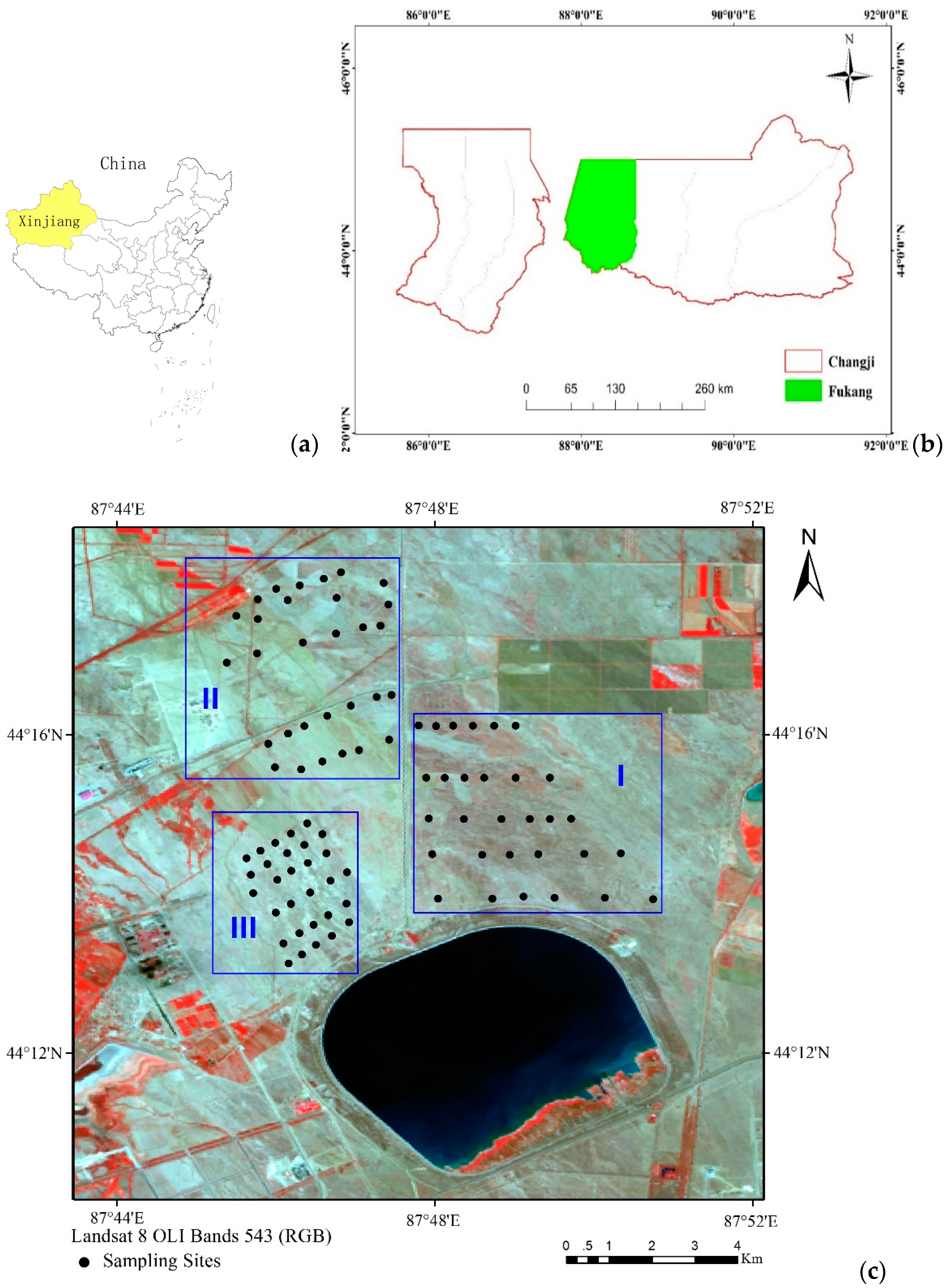
The sampling zone is divided into three types of soil zones according to the difference of human interference [25], as shown in Figure 1 (The blue rectangle is used to distinguish three different research areas), the Landsat 8 satellite acquisition date was in August 2017: ① light human interference zone (I Zone), here the soil basically keeps its the original state, and there is high vegetation coverage here, such as Haloxylon ammodendron, also the black biological crusts can be seen on the soil surface. ② moderate human interference zone (II Zone), here the wasteland soil was opened around the 1950s with 3 m width, but it was abandoned latter. Moreover, this zone is close to the 102th Regiment of Xinjiang, and there is relatively low vegetation coverage here compared with I Zone. ③ heavy human interference zone (III Zone), this zone has been reclaimed into two plantations with 3.5 m row spacing and 1.5 m plant spacing.
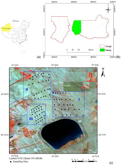
Figure 1.
Location map of sampling points: (a) location of China, (b) study area, and (c) sampling points.
2.2. Data Collection and Preprocessing
The field hyperspectral acquisition time was implemented in early October 2017 using ASD FieldSpec®3Hi-Res spectrometer with 350–2500 nm wavelength [26]. The time between 11:00 and 14:00 was selected as the measurement time, and it should be performed under cloudless and windless weather conditions. Furthermore, it was necessary to perform standard white calibration before each measurement, there was 15cm distance between the sensor and the soil surface, and the average hyperspectral value of the sample point was used as the spectral data of the sample point.
A soil auger was used to collect a soil sample with a depth of 0–20 cm, which was placed in a sealed bag and sent to laboratory, and a handheld GPS was adopted to record the latitude and longitude. At the same time, the surrounding environment and vegetation coverage of the sample site were photographed and recorded. The electrical conductivity method was used to determine the soil electrical conductivity (EC), which was then converted to soil salinity content.
The preprocessing method of hyperspectral data adopts the fractional-order derivative method [27,28], and the approximate formula for the definition of Grünwald–Letnikov (G–L) fractional-order derivative can been written as follows:
where, means soil hyperspectral signal, is the order of the derivative, and represents the memory length. represents the memory step length, and the value of h is 1, because the resampling interval of the ASD spectrometer is 1 nm. represents the Gamma function, it is .
2.3. Machine Learning Model
2.3.1. General Regression Neural Network
General Regression Neural Network (GRNN) was proposed by American scholar Specht D.F. in 1991, which is a new type of neural network based on nonlinear regression theory [29,30]. It can discover and continuously approximate the true value according to the implicit relationship in the sample data. Its advantage is that it has good approximation ability, recognition ability, and learning speed. There are few artificially adjusted parameters and only one threshold. Moreover, when the number of samples is small, the convergence of the output results and the results of the regression values are still considerable.
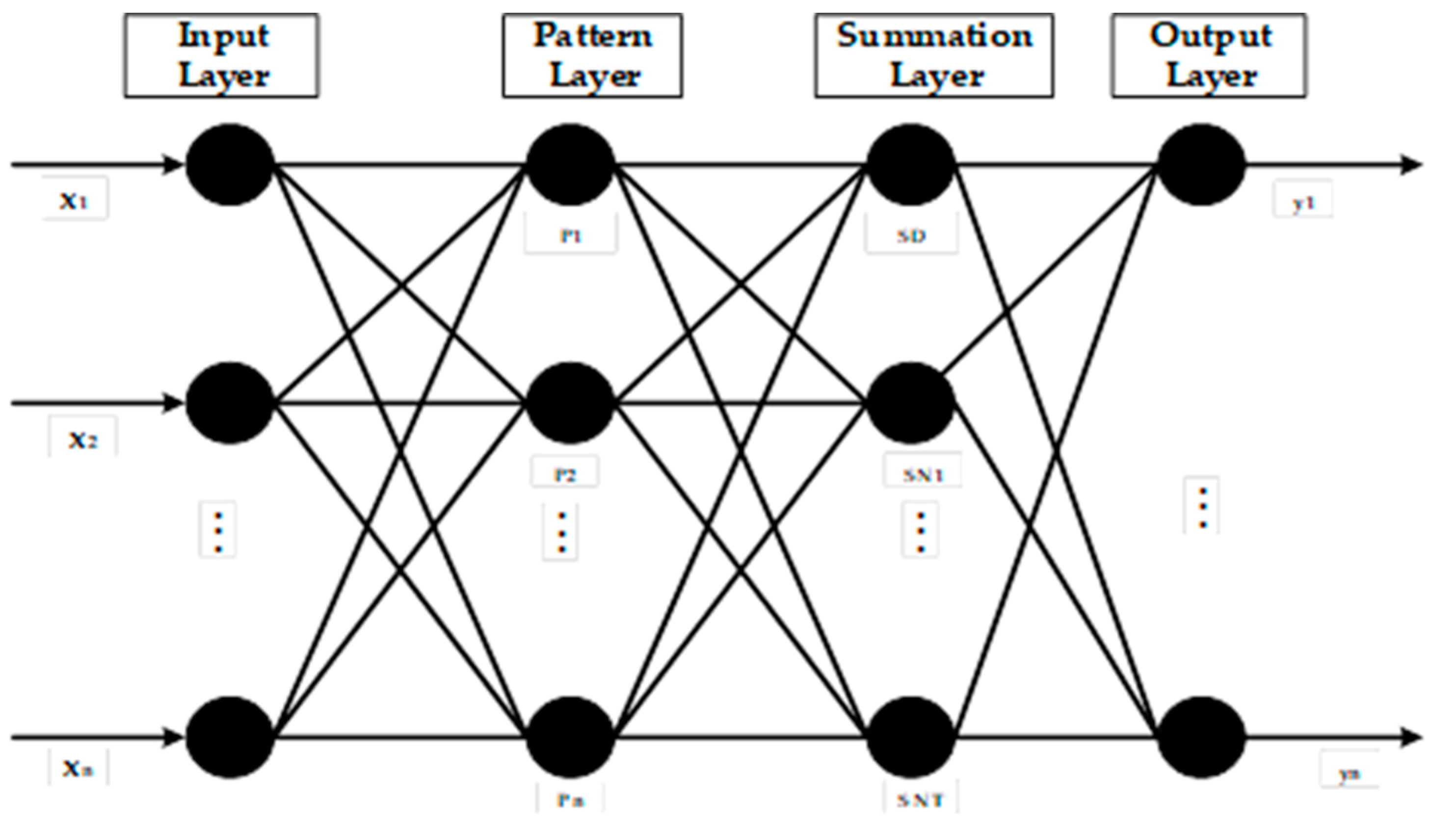
GRNN neural network is a kind of radial basis neural network based on mathematics statistics, which consists of four layers, namely the input layer, the pattern layer, the summation layer, and the output layer. Its network structure is shown in Figure 2.
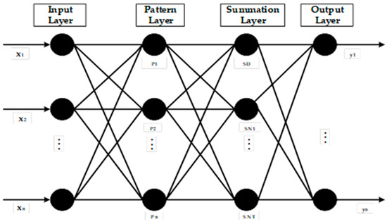
Figure 2.
Structure diagram of generalized regression neural network.
The theoretical basis of GRNN is as follows:
It can be assumed that and are two random variables, the joint probability density is . If the observed value of is known to be , then the regression value of relative to , that is, the conditional mean is:
is the predicted output of y under the condition that the input is , and the non-parametric estimation of Parzen can be used, the density function can be estimated from the sample data set according to Equations (3) and (4) as:
where, n is the sample size and p is the dimension of the random variable x. is the smoothing factor, which is the width coefficient of the Gaussian function. Substituting Equations (3) and (4) into Equation (2), and exchanging the order of integration and summation, we obtain
Because of , simplify the above Equation (5), we can obtain:
2.3.2. Extreme Learning Machine
The extreme learning machine (ELM) model uses the traditional three-layer neural network, but it is different from the traditional neural network. Traditional neural network learning algorithms (such as BP algorithm) need to set many network training parameters, and it is accompanied by more personal subjective factors in the setting process, so the repeatability of the model is poor, and the training speed is slow. ELM is a structure algorithm with a single hidden layer forward neuron network [31,32], which is superior to other traditional neural network learning algorithms in terms of learning speed and generalization performance. At the same time, it can use different excitation functions for sample training to overcome local minimal and inappropriate learning rate and other defects, making the training error to be minimized, optimizing the performance of the model.
2.3.3. Random Forest
Random forest (RF) model is a new type of machine learning method based on multiple decision tree theory [33,34]. RF is an ensemble learning algorithm that uses decision trees as weak learners and further introduces random attributes into the training of decision trees. When it is in the process of generating a new training set, the sample size contained in the decision tree will increase until it reaches the preset minimum number of nodes. The RF model can identify the complex non-linear relationship between the independent variable and the response variable, so that it has a high accuracy rate and a good anti-noise ability. When it is used to train high-dimensional data, the model has fast processing speed and does not require operations such as feature selection or data set normalization on the data.
2.4. Linear PLSR Model
Partial least squares regression (PLSR) is a multivariate linear analysis method, it can be used as model method when there is an obvious correlation between various variables and the number of experimental samples is less than the number of variables. This method is often used for quantitative analysis of spectra. Hyperspectral data has many bands, and there are problems of information redundancy and multicollinearity between the bands [35,36]. PLSR first uses principal component analysis in the modeling process to project spectral data onto a set of orthogonal factors that become latent variables and determine the optimal number of factors for the latent variables using internal cross-validation. The PLSR model can better solve the problem of multicollinearity between independent variables, achieve data dimensionality reduction, and eliminate unexplained noise. Therefore, it has been widely researched and applied in the hyperspectral remote sensing model.
2.5. Characteristic Band Selections
The hyperspectral imaging system can obtain the continuous spectral bands from visible light to near-infrared, and the number of bands reaches thousands. Therefore, continuous narrow bands will cause severe overlap of spectral information, and the spectral data collection process is subject to electromagnetic noise and other external interference. It will also cause a large amount of irrelevant redundant information between the spectral variables. If all these bands are used as the input variables of the model during process, it will cause a large amount of calculation work, as well as being time-consuming and labor-intensive, and will also lead to reduced model accuracy. Therefore, it is necessary to select effective wavelengths, reduce the number, and eliminate irrelevant variable information. This will be an important prerequisite for establishing the quantitative inversion of soil salt content information. It will play a role in reducing model complexity, exposing useful information, and improving model prediction ability and robustness.
2.5.1. Correlation Coefficient
Correlation coefficient (CC) analysis is a way to measure the relationship between variables and the strength of the relationship [37]. It plays a great role in sample data dimensionality reduction and missing value estimation. It is also the core tool of the current mainstream machine learning in preprocessing sample data. The Pearson correlation coefficient method proposed by statistician Carl Pearson is commonly used in hyperspectral data analysis, and its calculation formula is as follows:
where, is the correlation coefficient, is the band, is the spectral reflectance of the i-th band, is the sample content, and is the covariance of the two, and are the variance of the spectral reflectance and sample content ontent.
2.5.2. Competitive Adaptive Reweighted Sampling
Competitive adaptive reweighted sampling (CARS) imitates the principle of “survival of the fittest” in Darwin’s evolution theory. The method is based on Monte Carlo sample sampling, and each wavelength variable is regarded as an independent individual. Exponentially decreasing function (EDF) and adaptive reweighted sampling (ARS) are introduced to select variables [38,39,40]. The variable points with large absolute regression coefficients in PLSR are selected, and the variable points with smaller weights are eliminated. Cross-validation is used to select the subset of variables with the lowest root mean square error as the optimal combination of variables.
2.6. Model Evaluation Indicator
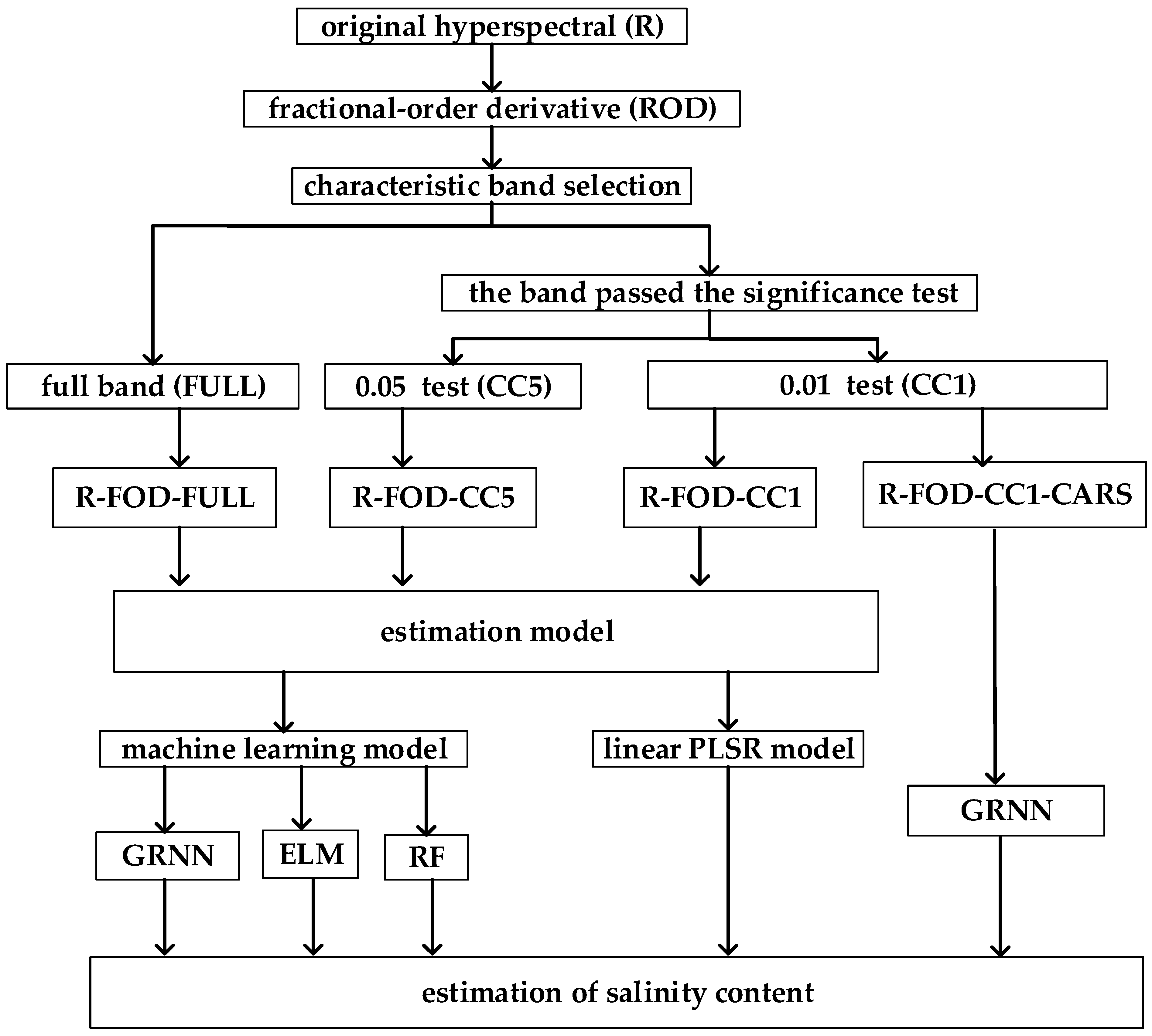
Characteristic band selection method is a crucial step for the establishment of soil salinity content prediction model. The goal of the characteristic band extraction is to discover the bands that have more ability to reveal the correlation between the spectroscopy and salinity. Therefore, four bands (R-FOD-FULL, R-FOD-CC5, R-FOD-CC1, and R-FOD-CC1-CARS represent the full band variables, the band passed the 0.05 significance test, the band passed the 0.01 significance test, and CC1 combined with CARS, respectively) have been choose as the input feature variables to develop the soil salinity estimation model. Finally, four models (GRNN, ELM, RF, and PLSR) were utilized to build the estimation model. The flow chart is shown in Figure 3.
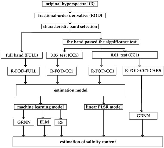
Figure 3.
Flow chart of the model.
Four models were applied to estimate the salinity for different research areas based on three bands (R-FOD-FULL, R-FOD-CC5, and R-FOD-CC1), and GRNN model was adopted to estimate the salinity based on R-FOD-CC1-CARS band. In this section, the sample points in the study zone are sorted according to the salinity content from high to low, the training set and the validation set are divided based on the principle of equal intervals, and 67% of the samples are selected for training, and the remaining 33% are for testing and validation. Meanwhile, all the estimation models of salinity content were performed using Matlab software (The MATHWORKS, Natick, MA, USA).
Three indicators are used to evaluate and compare the performance of the model [41,42,43], namely, root mean square error (RMSE), coefficient of determination (R2), and residual predictive deviation (RPD). When the RMSE value is small, and the R2 value is close to 1, indicating that the accuracy of the estimation model is higher. Meanwhile, RPD shows the estimation ability of the model by measuring the deviation degree between the estimated value and the measured value. When RPD ≥ 2.5, it indicated that the estimation performance is excellent. When 2.0 ≤ RPD < 2.5, it indicated that the estimation performance of this model is great. When 1.8 ≤ RPD < 2.0, it indicated that the estimation performance of this model is fine. When 1.4 ≤ RPD < 1.8, it indicated that the estimation performance of this model is general. When RPD < 1.4, it indicated that the model does not have estimation performance. Therefore, the best model usually exhibits the largest R2 and RPD values, and the lowest RMSE value.
where, represents the number of samples, represents the measured value of the i-th sample, represents the predicted value of the i-th sample, is the average of the measured values of the i-th sample, is the average of the predicted values of the i-th sample, SD is the standard deviation, and RMSE is the root mean square error.
3. Simulation Results
3.1. Correlation Coefficient Matrix Heat Map between Spectra and Salinity Based on Fractional-Order Derivative
The ground hyperspectral data is processed with fractional-order derivative (starting order is 0.0-order, ending order is 2.0-order, interval is 0.1, and a heat map of the correlation analysis between spectra and salinity is drawn (Figure 4)). Among them, the x-axis represents the range of the hyperspectral band, and the y-axis represents the order of the fractional-order derivative. What is more, the chromaticity bar on the right of the figure represents the size of the correlation coefficient, and the dark red (or dark yellow) area indicates that there is a high correlation coefficient between the spectrum and the salt.
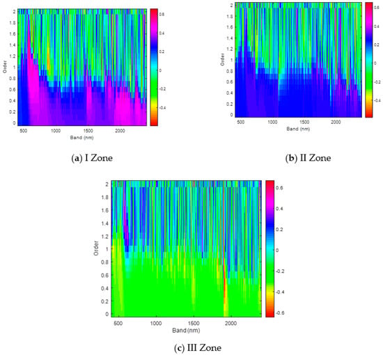
Figure 4.
Correlation coefficient matrix heat map between hyperspectral and salinity: (a) I Zone, (b) II Zone, and (c) III Zone.
Figure 4a reflects that the strong positive correlation peak in I Zone appears near 581nm, the corresponding fractional-order is 1.1 to 1.3 order, and the correlation coefficient is about 0.63. The simulation result in Figure 4b shows that the strong positive correlation peak in II Zone appears near 2213 nm, the corresponding fractional-order is 0.7 to 0.9 order, and the correlation coefficient is about 0.62. Figure 4c is the correlation analysis heat map of III Zone, which shows that a strong positive correlation peak appears near 551 nm, corresponding to the fractional-order of 1.5 to 1.7, and the correlation coefficient is about 0.65; meanwhile, the strong negative correlation peak appears near 2121 nm, the corresponding fractional order is 0.8 to 0.9 order, and the correlation coefficient is about −0.52.
In addition, when it is in the fractional order from 0 to 0.9, most of the wavelengths show a negative correlation in the III Zone, and the correlation coefficient value is about −0.3. While it shows a positive correlation in the I and II Zones, and the correlation coefficient value is about 0.4 in I Zone and about 0.2 in II Zone. When it is in the fractional order from 1 to 2, the correlation coefficient of ground hyperspectral and salinity exhibits relatively violent fluctuations in the three zones.
3.2. Estimation of Salinity Based on Full Band
The results of estimating the salt content based on all band models are shown in Table 1. The calculation process is: first, calculate the FOD of the soil original hyperspectral based on all bands; then, use the hyperspectral reflectance of all bands at different FOD as the independent variable, the total salt content as the dependent variable, and use four models (PLSR, GRNN, ELM, and RF) to estimate the total salt content; finally, find the optimal estimation model based on FOD in each zone.

Table 1.
Accuracy analysis of salinity estimation based on all band models.
Regardless of the human interference area, because the R-FOD-FULL model uses all bands (that is 1759) for modeling, there are many independent variables, and the amount of redundant information between bands is large. The RPD values of the three models (PLSR, ELM, and RF) predict total salt are less than 1.0, which cannot quantitatively predict the total salt content of the soil. Moreover, the R-FOD-FULL-GRNN model has a general effect on the prediction of total salt in III Zone (RPD is between 1.4 and 1.8), but the model does not have the ability to predict the total salt content in I Zone and II Zone.
3.3. Estimation of Salinity Based on a Characteristic Band Model with a Significance Level of 0.05
The estimation performance of the salt content based on the 0.05 significance level is shown in Table 2, the scatter plots of the salt content between measured and estimated values are shown in Figure 5, and the characteristic bands selected by different models are shown in Figure 6. The calculation process is as follows: First preprocess the original hyperspectral data of the soil by FOD. Then, analyze the correlation between the hyperspectral and soil salinity, and use the band passed the 0.05 significance level as the characteristic band (R-FOD-CC5). Finally, establish four prediction models (PLSR, GRNN, ELM, and RF) to estimate the salt content, and select the best prediction model in each zone.
Table 2.
Accuracy analysis of salinity estimation based on feature band models under 0.05 significance level.
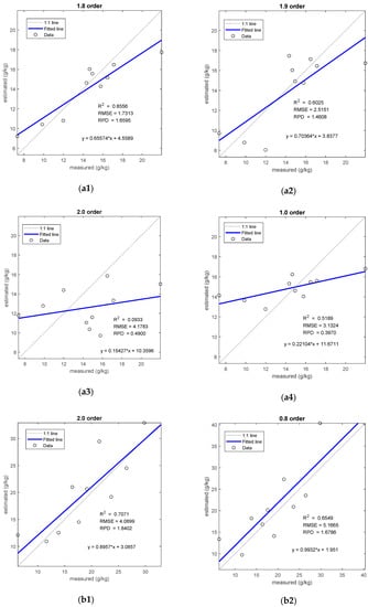
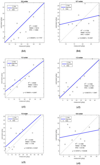
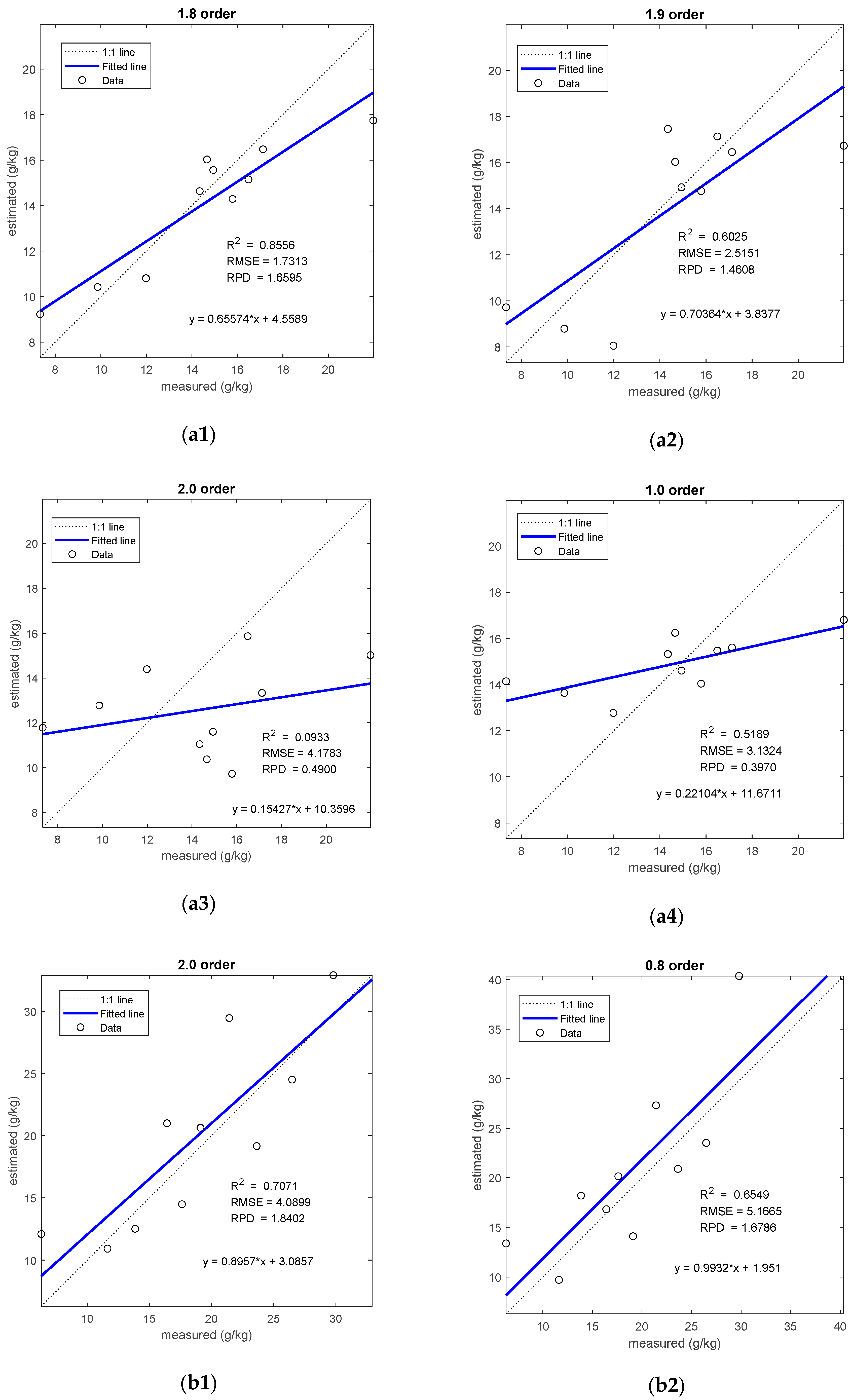
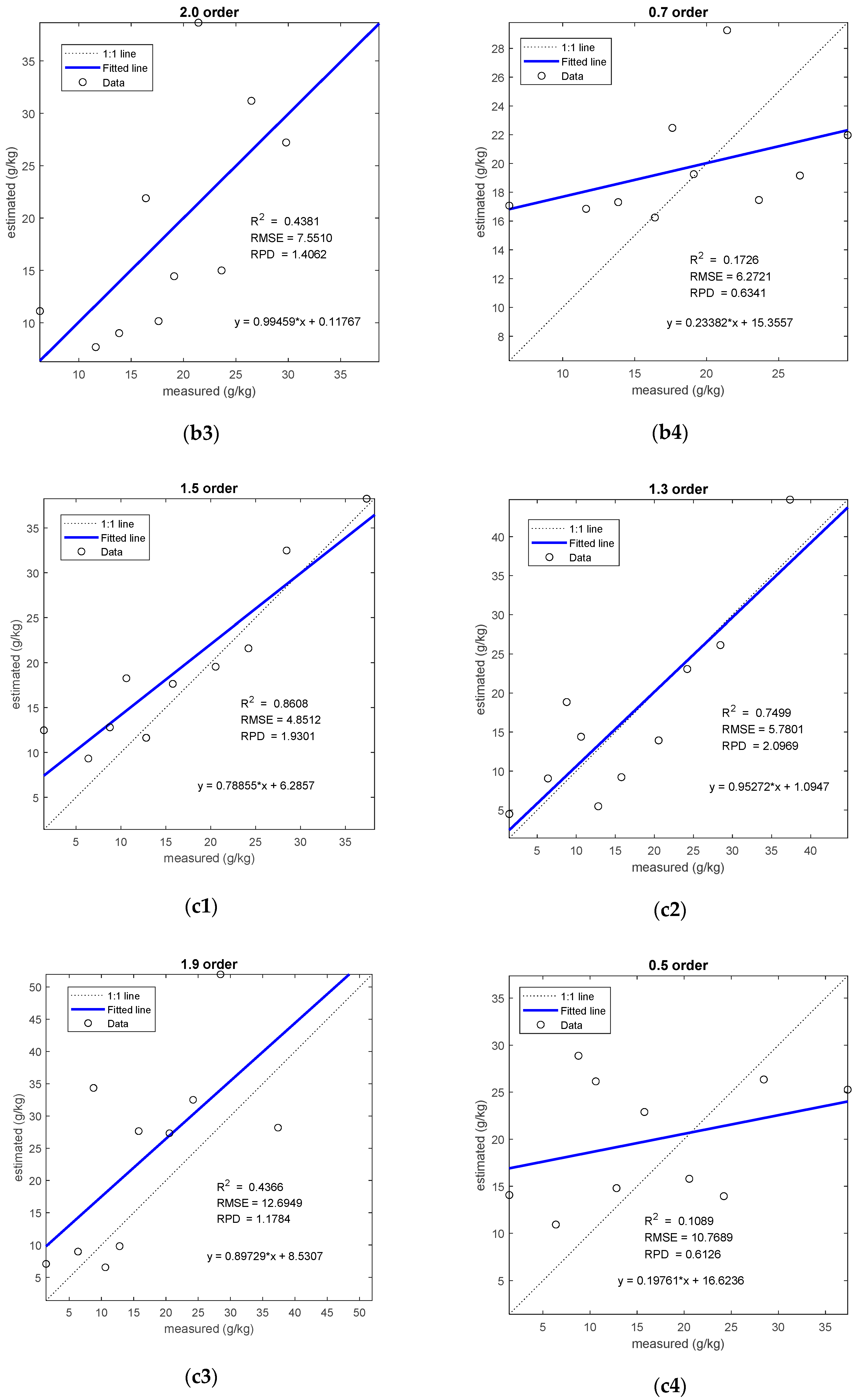
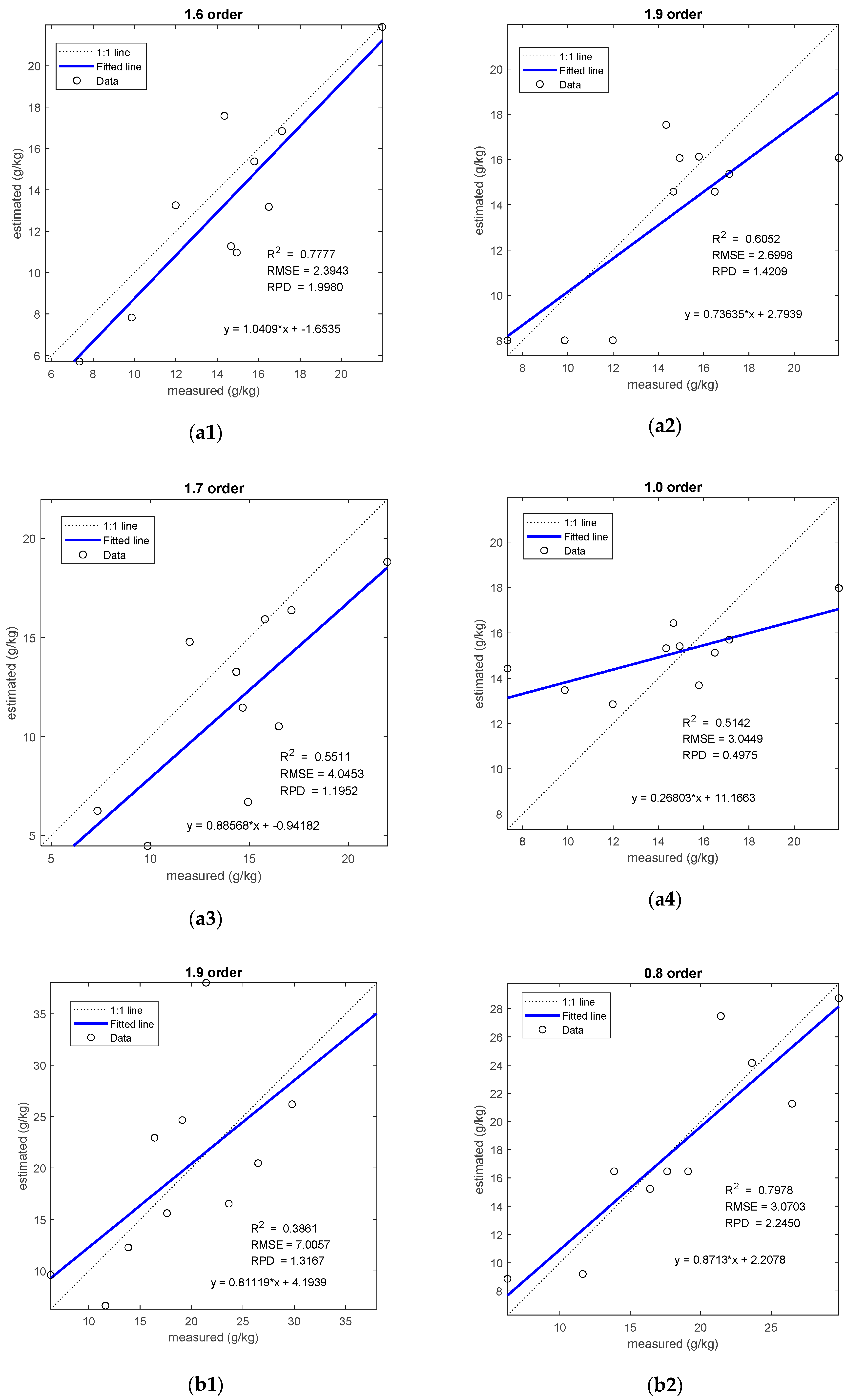
Figure 5.
Comparisons of measured and estimated salt contents based on different models of validation set: (a1) I Zone of PLSR, (a2) I Zone of GRNN, (a3) I Zone of ELM, and (a4) I Zone of RF; (b1) II Zone of PLSR, (b2) II Zone of GRNN, (b3) II Zone of ELM, and (b4) II Zone of RF; (c1) III Zone of PLSR, (c2) III Zone of GRNN, (c3) III Zone of ELM, and (c4) III Zone of RF.

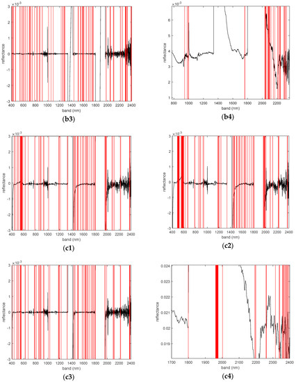
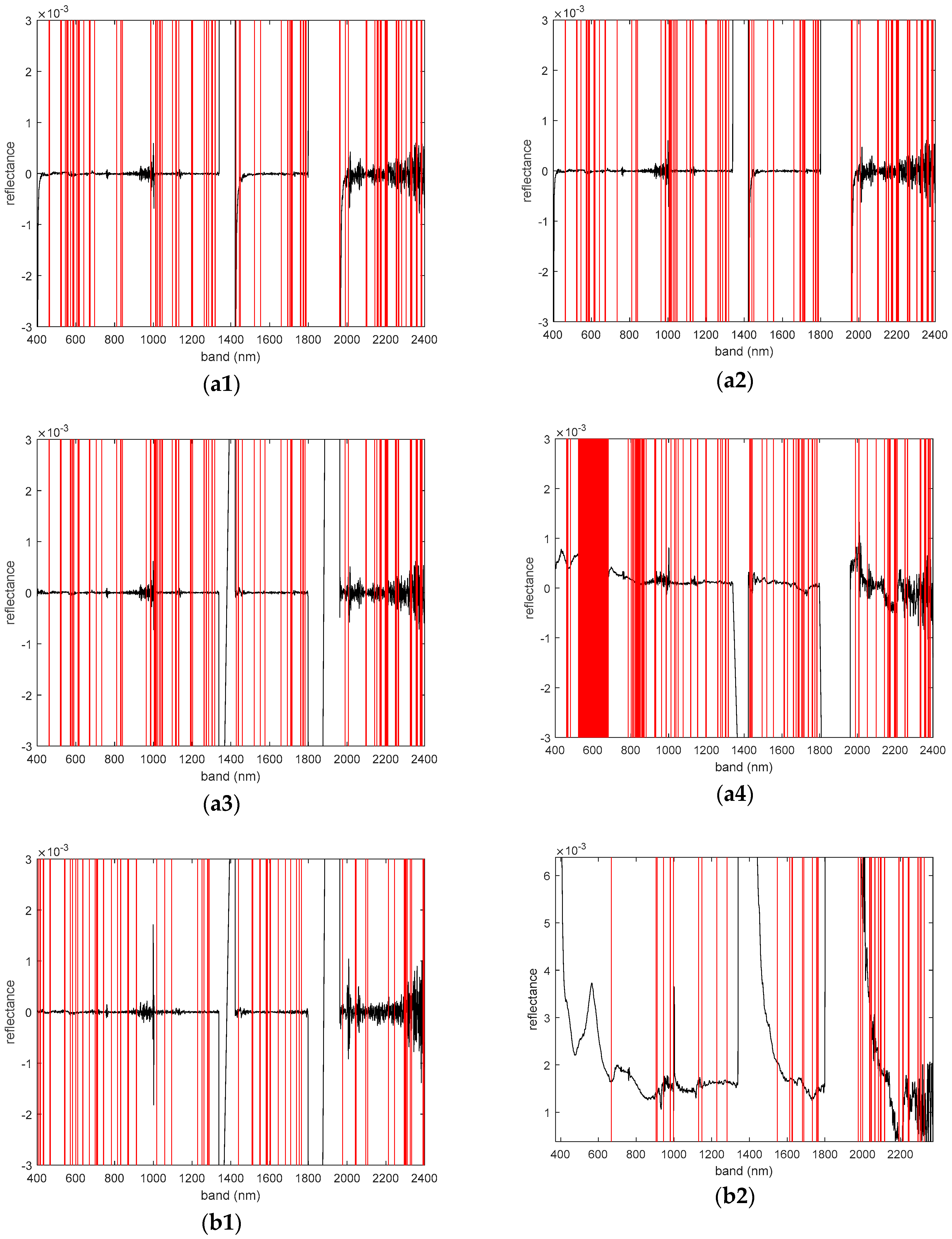
Figure 6.
Number of characteristic bands selected in different models: (a1) I Zone of PLSR, (a2) I Zone of GRNN, (a3) I Zone of ELM, and (a4) I Zone of RF; (b1) II Zone of PLSR, (b2) II Zone of GRNN, (b3) II Zone of ELM, and (b4) II Zone of RF; (c1) III Zone of PLSR, (c2) III Zone of GRNN, (c3) III Zone of ELM, and (c4) III Zone of RF.
3.3.1. Performance Analysis for Estimating Salinity
Compared with the R-FOD-FULL model, the R-FOD-CC5 model has a significant improvement in the prediction effect of salt content. This is because the number of characteristic band variables selected based on R-FOD-CC5 is reduced compared to R-FOD-FULL. However, there is still a certain degree of redundancy between the characteristic band variables selected based on R-FOD-CC5, which has a greater impact on the subsequent model construction and accuracy fitting.
For the machine learning model, regardless of the degree of human interference, the optimal model for estimating the salt content is based on the R-FOD-CC5-GRNN model established by GRNN, and it located in the fractional order (I Zone is 1.9 order, II Zone is 0.8 order, and III Zone is 1.3 order), all the RPD values are both greater than 1.4. The prediction capabilities of these models for I Zone and II Zone have reached a general level, and the prediction capabilities for Zone III have reached a great level. Among them, the R2, RMSE, and RPD values of the verification set are, respectively, 0.6025, 2.5151, and 1.4608 in I Zone; it is 0.6549, 5.1665, and 1.6786 in II Zone; it is 0.7499, 5.7801, and 2.0969 in III Zone. However, the R-FOD-CC5-RF model based on RF cannot estimate the soil salt content of the three zones, and its RPD is less than 1.0, and the R-FOD-CC5-ELM model based on ELM cannot quantitatively estimate the soil salt content of I Zone and III Zone, but it can estimate the soil salt content of II Zone, and the prediction performance is general.
Regarding the linear prediction model, the R-FOD-CC5-PLSR model based on PLSR has a better effect on total salt prediction. The R2 and RMSE of the verification set are 0.8556, 1.7313, and 1.6595 in I Zone; it is 0.7071, 4.0899, and 1.8402 in II Zone; it is 0.8608, 4.8512, and 1.9301 in III Zone. Therefore, the prediction performance of this model for I Zone is general, and the prediction performance for II and III Zone is fine.
In summary, the R-FOD-CC5-GRNN model has the best prediction effect on III Zone, while the R-FOD-CC5-PLSR model has the best prediction effect on I and II Zone, but the features bands selected in III, II, and I Zone are 103, 80, and 112, respectively, accounting for 5.86%, 4.55%, and 6.37% of the full-band. This reflects that the number of characteristic bands is still redundant, and redundant bands need to be deleted to further improve the accuracy of the prediction model.
3.3.2. Test Results of Different Models
Comparation of measured and estimated value of soil salt content in validation set is shown in Figure 5.
The comparison model based on the machine learning is shown in Figure 5a2–a4,b2–b4,c2–c4. The predicted value of the RF model differs greatly from the measured value on the 1:1 line, and the data points have a high degree of dispersion. The ELM model predicts that the dispersion of data points in I and III Zone is also high, while the dispersion of data points in II Zone is low. The GRNN model has a fine fitting effect on I and II Zone, and a great fitting effect on III Zone, and the coefficient of determination of the fitting equation is 0.7499, the fitting equation is y = 0.95272 ∗ x + 1.0947.
The comparison model based on the linear PLSR is shown in Figure 5a1,b1,c1. The fitting line of the data points has a high degree of coincidence with the 1:1 line, and the R-FOD-CC5-PLSR model also performs well in the fitting effect of I, II, and III Zone. The coefficients of determination of the fitting equations are 0.8556, 0.7071 and 0.8608, respectively, and the fitting equations are, respectively, y = 0.65574 ∗ x + 4.5589, y = 0.8957 ∗ x + 3.0857, and y = 0.78855 ∗ x + 6.2857.
3.3.3. Characteristic Bands Selected by Different Models
The characteristic bands selected by different models are shown in Figure 6.
For machine learning models in I, II, and III Zone, the number of characteristic bands selected by the GRNN-based optimal model are 111, 62, and 103, respectively, accounting for 6.31%, 3.52%, and 5.86% of all bands. The number of characteristic bands selected by the ELM-based optimal model are 107, 80, and 76, respectively, accounting for 6.08%, 4.55%, and 4.32% of all bands. The number of characteristic bands selected by the RF-based optimal model are 277, 48, and 40, respectively, accounted for 15.75%, 2.73%, and 2.27% of all bands.
The number of characteristic bands selected by the linear-based PLSR model in I, II, and III Zone are 112, 80, and 82, respectively, accounting for 6.37%, 4.55%, and 4.66% of all bands.
3.4. Estimation of Salinity Based on a Characteristic Band Model with a Significance Level of 0.01
The comparison of the estimation accuracy of the four models (PLSR, GRNN, ELM, and RF) for predicting salt content is shown in Table 3, the test results of different models are shown in Figure 7, and the characteristic bands of the optimal model are shown in Figure 8. The calculation process is: First, use the fractional-order derivative method to preprocess the original hyperspectral data of the soil. Then, calculate the correlation between the spectrum and the salinity in the three interference regions, and use the band passed the 0.01 significance level as the characteristic band variable (R-FOD-CC1), these characteristic band variables are used as independent variables, and the salt content is used as the dependent variable. Finally, four estimation models (PLSR, GRNN, ELM, and RF) are established, and each optimal estimation model in each region is selected.
Table 3.
Accuracy analysis of salinity estimation based on feature band models under 0.01 significance level.
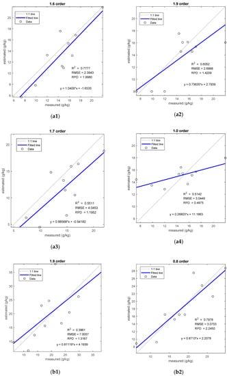
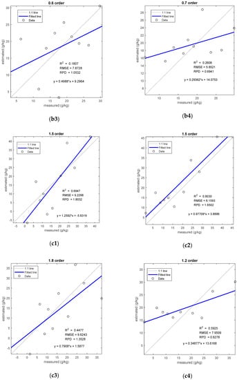
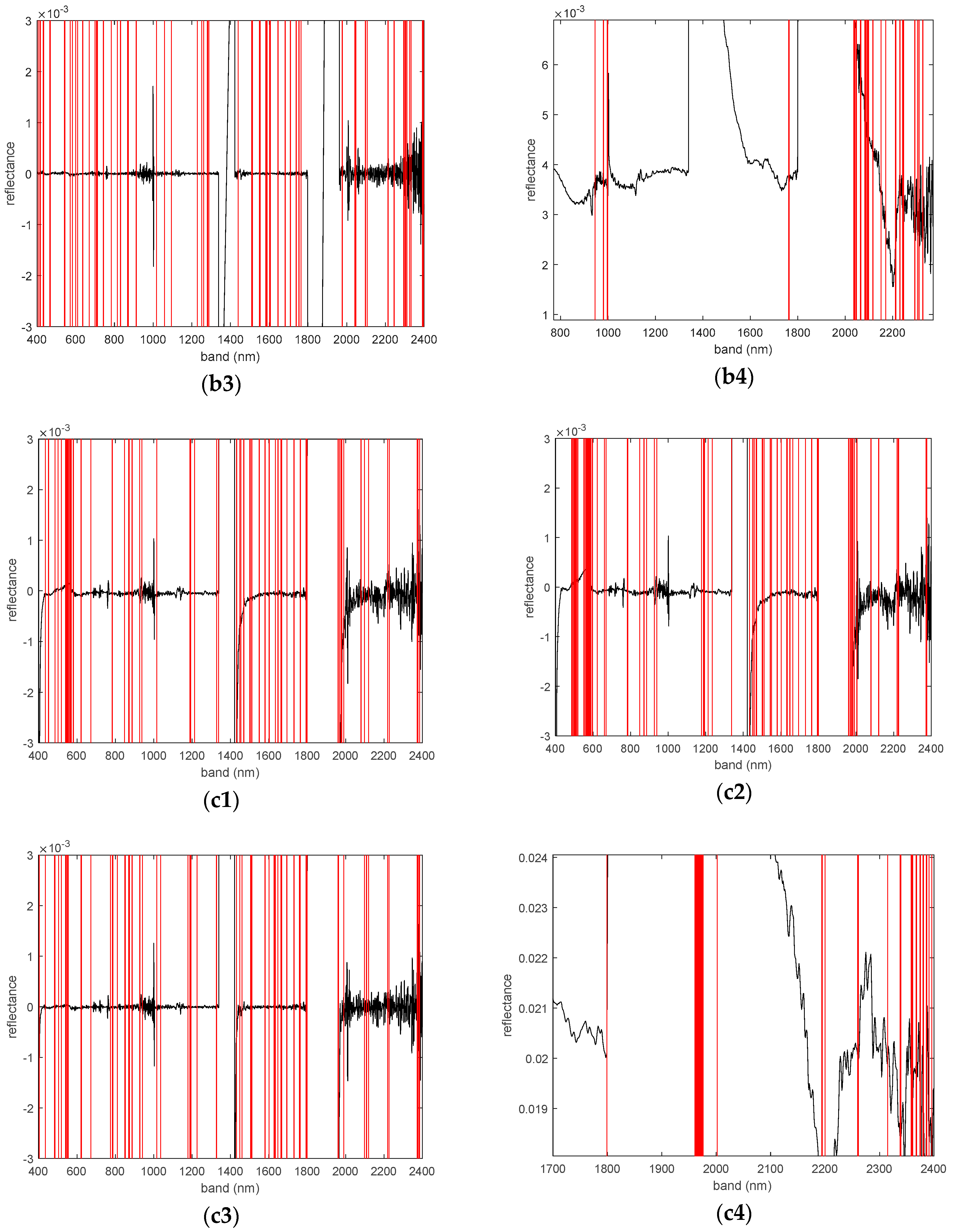
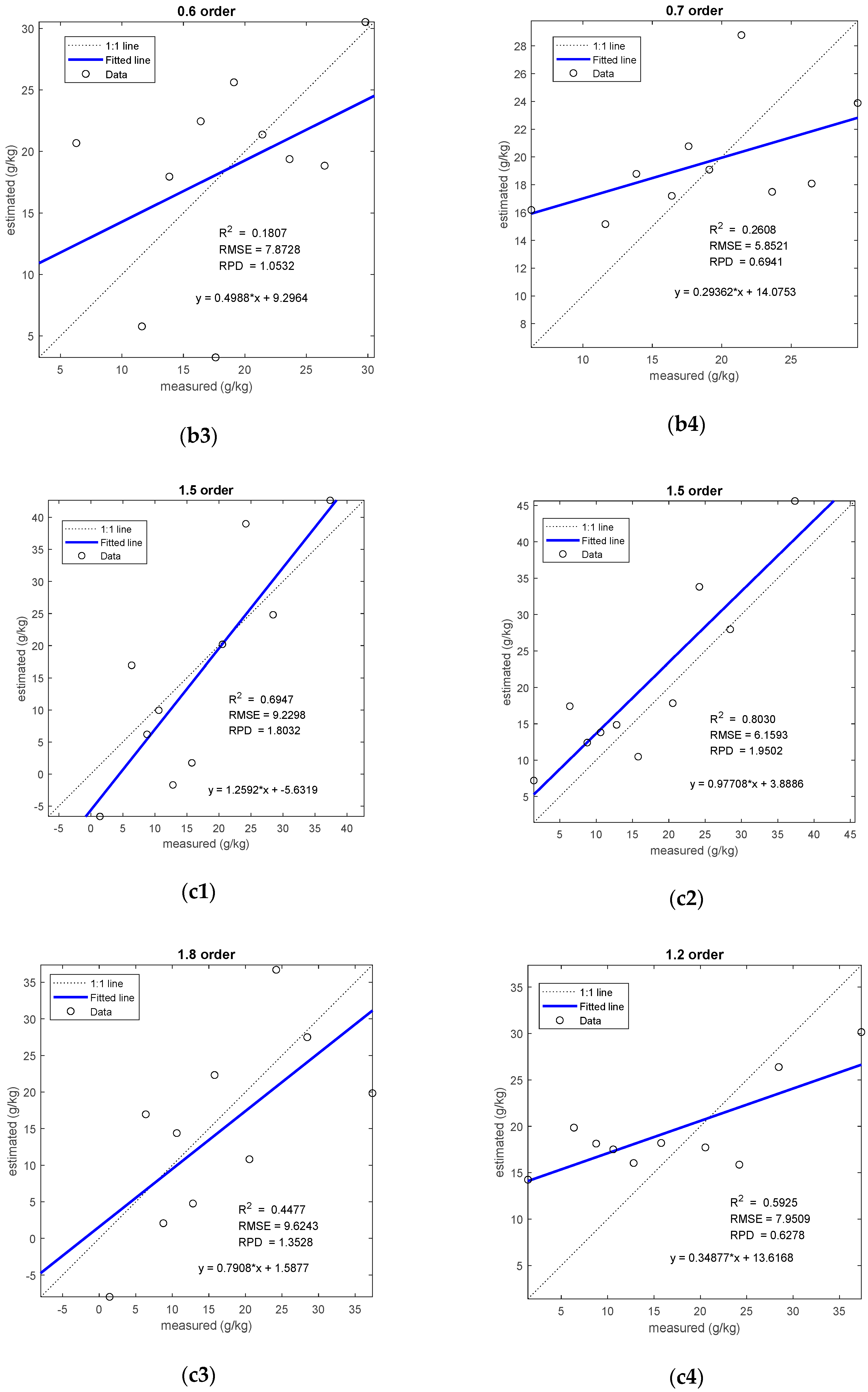
Figure 7.
Comparisons of measured and estimated salt contents based on different models of validation set: (a1) I Zone of PLSR, (a2) I Zone of GRNN, (a3) I Zone of ELM, and (a4) I Zone of RF; (b1) II Zone of PLSR, (b2) II Zone of GRNN, (b3) II Zone of ELM, and (b4) II Zone of RF; (c1) III Zone of PLSR, (c2) III Zone of GRNN, (c3) III Zone of ELM, and (c4) III Zone of RF.
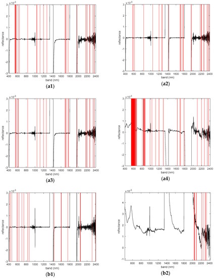
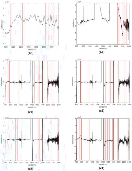
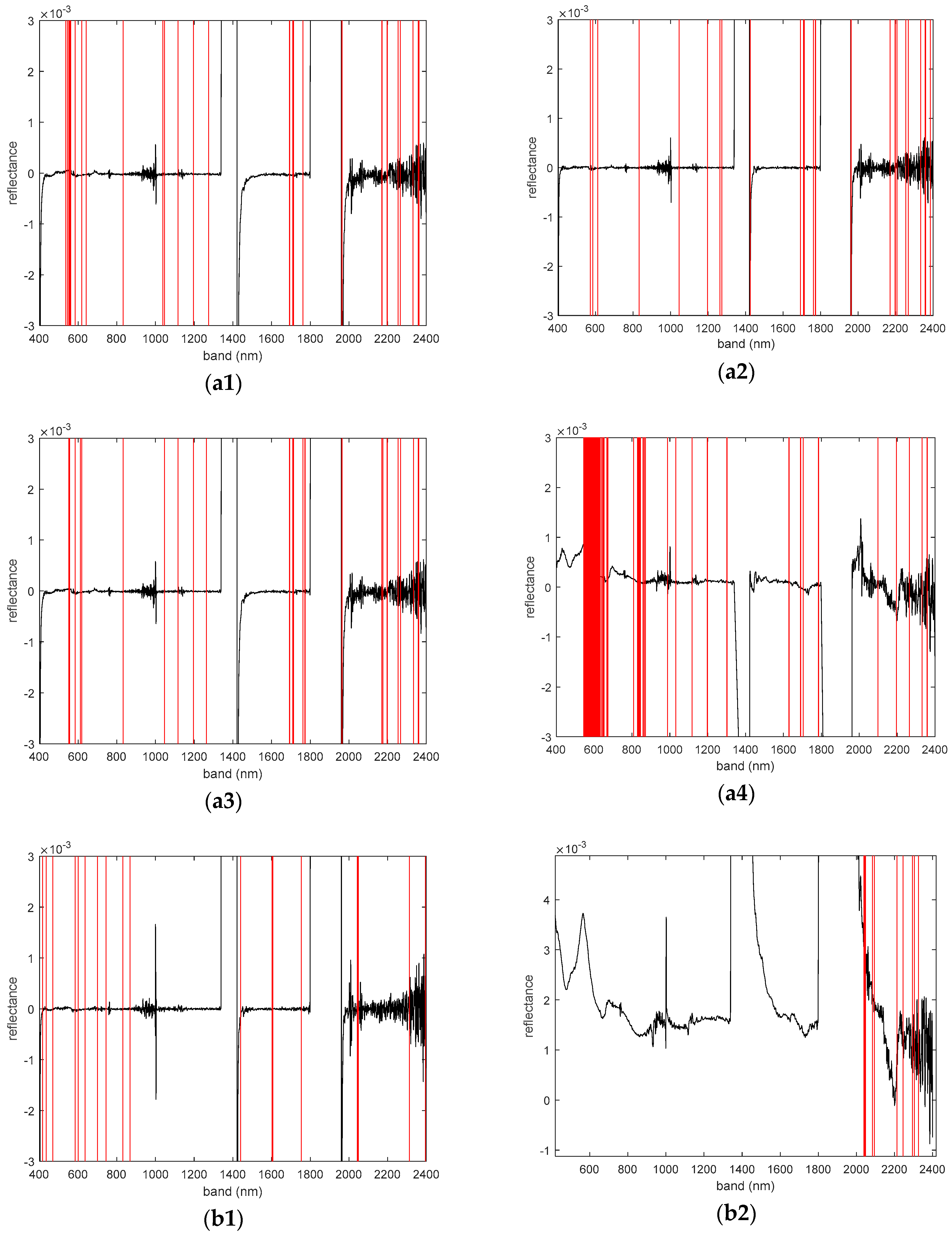
Figure 8.
Number of characteristic bands selected in different models: (a1) I Zone of PLSR, (a2) I Zone of GRNN, (a3) I Zone of ELM, and (a4) I Zone of RF; (b1) II Zone of PLSR, (b2) II Zone of GRNN, (b3) II Zone of ELM, and (b4) II Zone of RF; (c1) III Zone of PLSR, (c2) III Zone of GRNN, (c3) III Zone of ELM, and (c4) III Zone of RF.
3.4.1. Accuracy Comparison of Salt Estimation
Compared with the R-FOD-CC5 model, the prediction effect of the R-FOD-CC1 model on the salt content is greatly improved. The reason is that the number of feature band variables extracted is less, and the redundancy between the bands is smaller, which makes the prediction accuracy of the estimation model higher.
In I Zone, the optimal model for estimating salinity is R-FOD-CC1-PLSR. The R2, RMSE, and RPD of this model in the verification set are 0.7777, 2.3943, and 1.9980, and its predictive performance for the salt in I Zone is fine. Meanwhile, the optimal model appears in the 1.6 order, and the number of selected characteristic band variables is 33, accounting for 1.88% of the full band. However, the performance of the model based on GRNN to predict the salt content of I Zone is general, and its RPD value is between 1.4 and 1.8. The estimation model based on ELM and RF has poor predictive performance, because the RPD value is less than 1.4, it cannot predict the salt content in I Zone.
In II Zone, the R-FOD-CC1-GRNN model based on GRNN has the best estimation results, the R2, RMSE, and RPD in the verification set are 0.7978, 3.0703, and 2.2450, and this model has fine performance in predicting the salt content in II Zone. Moreover, the fractional order is 1.8, and 13 bands are selected as characteristic band variables, accounting for 0.74% of the full band. Nevertheless, the remaining three models (PLSR, ELM, and RF) have poor performance in estimating the salt content in II Zone, and the RPD in II Zone is 1.3167, 1.0532, and 0.6941, respectively.
In III Zone, the R-FOD-CC1-GRNN model has the best effect in estimating total salt. The R2, RMSE, and RPD in the verification set are 0.8030, 6.1593, and 1.9502, since the RPD value of this model is between 1.8 and 2.0, the estimation performance of this model for the total salt content can reach a fine level. In addition, the number of characteristic band variables of the optimal model is 18, accounting for 1.02% of the full band, and it appears in the 1.5 fractional order. However, the ELM and RF models cannot estimate the soil salt content in III Zone because the PRD values of the model in the verification set are all less than 1.4. Meanwhile, because the RPD value of the PLSR model is greater than 1.8, it has a fine performance in predicting the salt content, and it can quantitatively estimate the salt content, the R2, RMSE, and RPD in the R-FOD-CC1-PLSR model are 0.6947, 9.2298, and 1.8032, while they are 0.8030, 6.1593, and 1.9502 in the R-FOD-CC1-GRNN model. So, it can be seen that the R2 value and RPD value are larger in the R-FOD-CC1-GRNN model, and the RMSE value is smaller. Therefore, the best model for predicting the soil salt content in III Zone is R-FOD-CC1-GRNN.
3.4.2. Validation of Optimal Salt Model
The test results of the four models based on R-FOD-CC1 to estimate the salt content in the three regions are shown in Figure 7.
The data points of the R-FOD-CC1-PLSR model in I Zone are more evenly distributed on both sides of the fitting line, R2 is 0.7777, the degree of fit is fine, and the fitting equation is expressed as y = 1.0409 ∗ x + (−1.6535). The best model for testing the salt content in II Zone is R-FOD-CC1-GRNN, the data points are distributed evenly on both sides of the fitting line, R2 is 0.7978, and the fit is great, and the fitting equation is expressed as y = 0.8713 ∗ x + 2.2078. The R-FOD-CC1-GRNN model has the best effect in testing the salt content of III Zone, R2 is 0.8030, and the fit is fine, the fitting equation is expressed as y = 0.97708 ∗ x + 3.8886.
It can be seen from Figure 5 and Figure 7 that compared with the R-FOD-CC5 model as a whole, the characteristic band model based on R-FOD-CC1 can effectively reduce the number of modeled band variables, simplify the model structure, its measured and estimated values are more evenly distributed near the 1:1 line, the prediction accuracy of these model is higher, and the soil salt content can be estimated more accurately.
3.4.3. The Characteristic Band of the Optimal Model
The characteristic bands selected by the four estimation models (PLSR, GRNN, ELM, and RF) in the three regions are shown in Figure 8. The number of characteristic bands selected in I Zone for R-FOD-CC1-PLSR, R-FOD-CC1-GRNN, R-FOD-CC1-ELM, and R-FOD-CC1-RF models are 33, 25, 25, and 112, respectively, they account for 1.88%, 1.42%, 1.42%, and 6.37% of the full bands, respectively. The number of bands selected in II Zone are 18, 13, 8, and 12, respectively, which account for 1.02% and 0.74%, 0.45%, and 0.68% of the full bands, respectively. The number of bands selected in III Zone are 18, 18, 12, and 22, respectively, which account for 1.02%, 1.02%, 0.68%, and 1.25% of the total number of bands, respectively.
The characteristic band variables selected by most models appear in both visible light and near infrared. However, the characteristic band of II Zone for R-FOD-CC1-GRNN model and R-FOD-CC1-RF model only appear near infrared. The R-FOD-CC1-PLSR model has the best effect in estimating soil salinity in I Zone, the 33 band variables selected are concentrated around 600 nm, 1100 nm, and 2300 nm in Figure 8a1.
The R-FOD-CC1-GRNN model predicts that the soil salinity in II Zone has the best performance, the 13 characteristic band variables are concentrated in the near infrared band near 2200 nm in Figure 8b2. Figure 8c2 shows that the characteristic band selected by the R-FOD-CC1-GRNN model to estimate soil salinity in III Zone mainly appear in the vicinity of 555 nm, 1700 nm and 2000 nm.
3.5. Estimation of Salinity Based on R-FOD-CC1-CARS-GRNN Model
From the simulation results in Section 3.2, Section 3.3 and Section 3.4, it can be seen that the accuracy of the GRNN machine learning model for predicting salinity is higher than that of the ELM and RF. Although the number of feature bands extracted based on the CC1 method is less, but R-FOD-CC1-GRNN has low prediction accuracy for I Zone, and the number of feature bands extracted by the model in I, II, and III Zone are 25, 13, and 18, respectively. It indicates that the number of characteristic bands selected based on the CC1 method is more than 12, and the feature bands need to be further screened using CARS method, it is expected to improve the model performance in the three zones. So, the R-FOD-CC1-CARS-GRNN model has been proposed.
The calculation process of R-FOD-CC1-CARS-GRNN model is: First, use FOD to preprocess the original hyperspectral data. Then, adopt CARS method to extract the characteristic band based on the CC1 band, so as to further reduce the dimensionality of the CC1 band variable in order to find the sensitive band variable of salinity. Finally, employ GRNN model to estimate the salt content, and the optimal fractional-order model will be selected in each zone.
3.5.1. Inversion Results of Salt Estimation
The estimation accuracy of salinity based on R-FOD-CC1-CARS bands using GRNN models is shown in Table 4.
Table 4.
Inversion results of salt estimation based on R-FOD-CC1-CARS-GRNN compared with CC1-GRNN and CC1-PLSR.
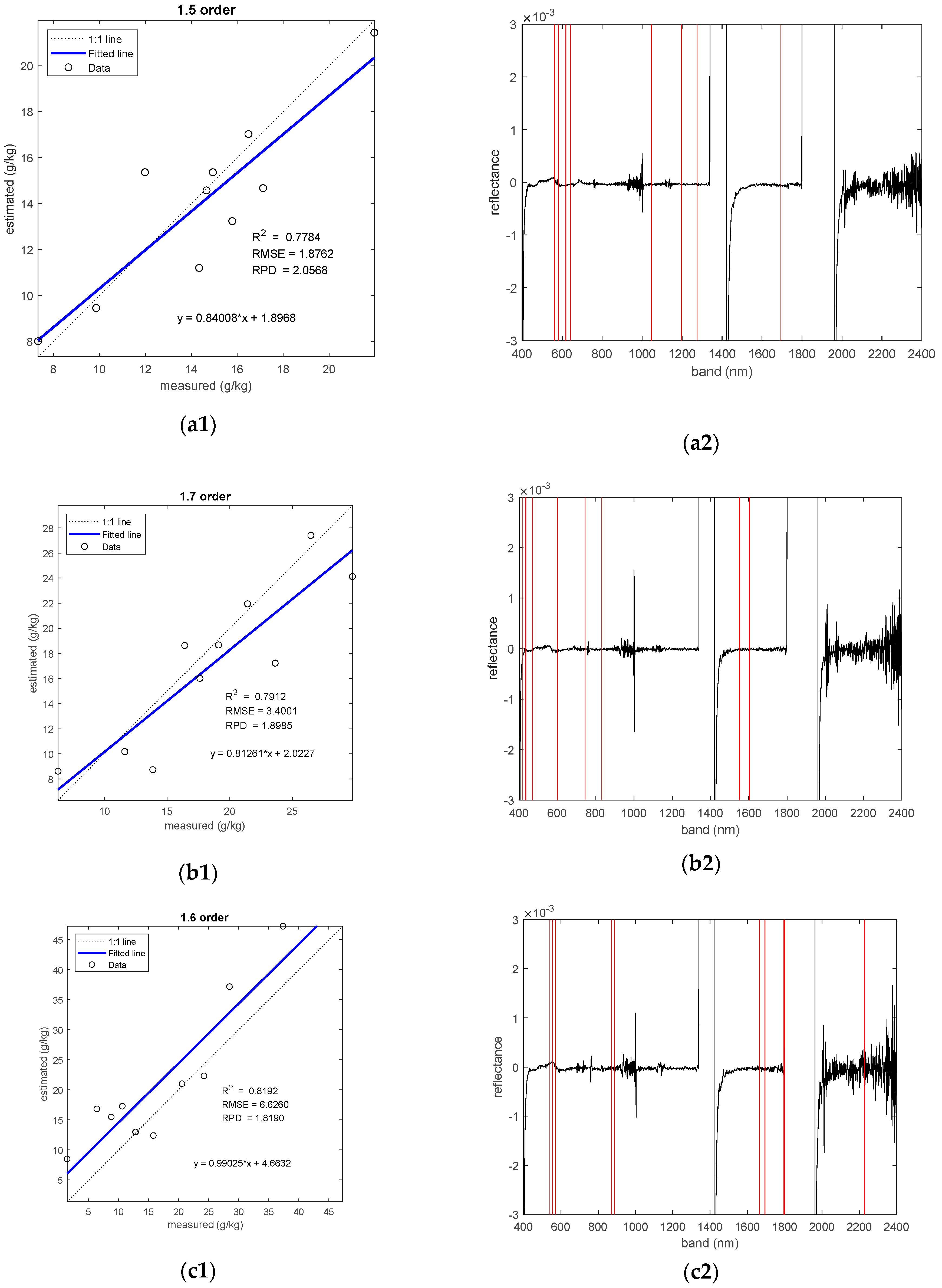
Compared with Table 1, Table 2 and Table 3, the results of Table 4 show that the model based on R-FOD-CC1-CARS-GRNN has fewer input variables, which simplifies the complexity and redundancy of the model. What is more, the optimal models of I, II, and III Zone are 1.5, 1.7, and 1.6 fractional-order, respectively; the number of characteristic bands are 8, 9, and 11, respectively, which account for 0.45%, 0.51%, and 0.63% of the full wave wavelength, respectively. The R2, RMSE, and RPD of the model is 0.7784, 1.8762, and 2.0568 in I Zone; it is 0.7912, 3.4001, and 1.8985 in II Zone; it is 0.8192, 6.6260, and 1.8190 in III Zone. The predictive ability of the model for I Zone is great, the predictive ability for II and III Zone are all fine.
In I Zone, compared with R-FOD-CC1-GRNN and R-FOD-CC1-PLSR model, R-FOD-CC1-CARS-GRNN model has the smallest RMSE, the largest R2 and RPD, and the smallest number of characteristic bands. Therefore, the optimal model for estimating salinity is R-FOD-CC1-CARS-GRNN.
In II Zone, compared with the R-FOD-CC1-PLSR model, the R-FOD-CC1-CARS-GRNN model has a smaller RMSE, a larger R2 and RPD, and a smaller number of characteristic bands. Compared with the R-FOD-CC1-GRNN model, although the R-FOD-CC1-CARS-GRNN model has a smaller RPD than the former, its R2 and RMSE are close to the former, and the former has more characteristic bands than the latter. At the same time, the optimal order of the latter appears at 1.7, while the optimal order of the latter appears at 0.8. Studies by scientists have shown that higher-order FOD are more effective in predicting soil properties. Therefore, when comprehensively considering the model accuracy index and the number of characteristic bands, the optimal model that should be selected is R-FOD-CC1-CARS-GRNN.
In III Zone, compared with R-FOD-CC1-PLSR, the R-FOD-CC1-CARS-GRNN model has the largest RPD and R2, it also has the smallest RMSE. Compared with R-FOD-CC1-GRNN, the R-FOD- CC1-CARS-GRNN model has the largest R2, its RPD and RMSE value are close to the former, and the number of characteristic bands for the latter is less than that of the former, which greatly reduces the calculation time. Therefore, the optimal model for predicting soil salinity in III Zone is R-FOD-CC1-CARS-GRNN.
Therefore, it can be known from Table 4 that the optimal model for the three zones is R-FOD-CC1-CARS-GRNN by comprehensively analyzing the model evaluation indicator and the number of characteristic bands. The number of characteristic band variables is small, there are 8 (562, 581, 618, 641, 1046, 1197, 1275, and 1694 nm) in I Zone, 9 (418, 434, 469, 600, 744, 831, 1551, 1603, and 1604 nm) in II Zone, and 11 (541, 555, 556, 570, 872, 886, 1663, 1694, 1795, 1799, and 2227 nm) in III Zone, which greatly reduces the modeling time. The simulation results show that the R-FOD-CC1-CARS-GRNN model can effectively realize the quantitative prediction of the salt content in the soil, and the coupling algorithm of CC1 combined with CARS can reduce the number of modeling variables and improve the accuracy of the model, indicating the coupling of the two can be used as an effective method for variable optimization, and can provide a reference for the characteristic bands screening of other soil properties using soil hyperspectral reflectance.
3.5.2. Validation Result and Feature Band of the Best Model
It is needed to verify the prediction set based on R-FOD-CC1-CARS-GRNN model, and the validation results and the feature bands selected by CARS of the best R-FOD-CC1-CARS-GRNN model is shown in Figure 9.
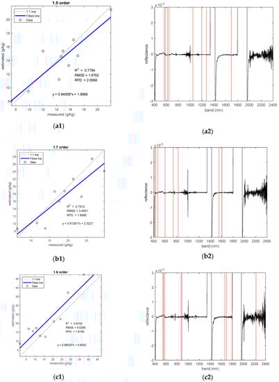
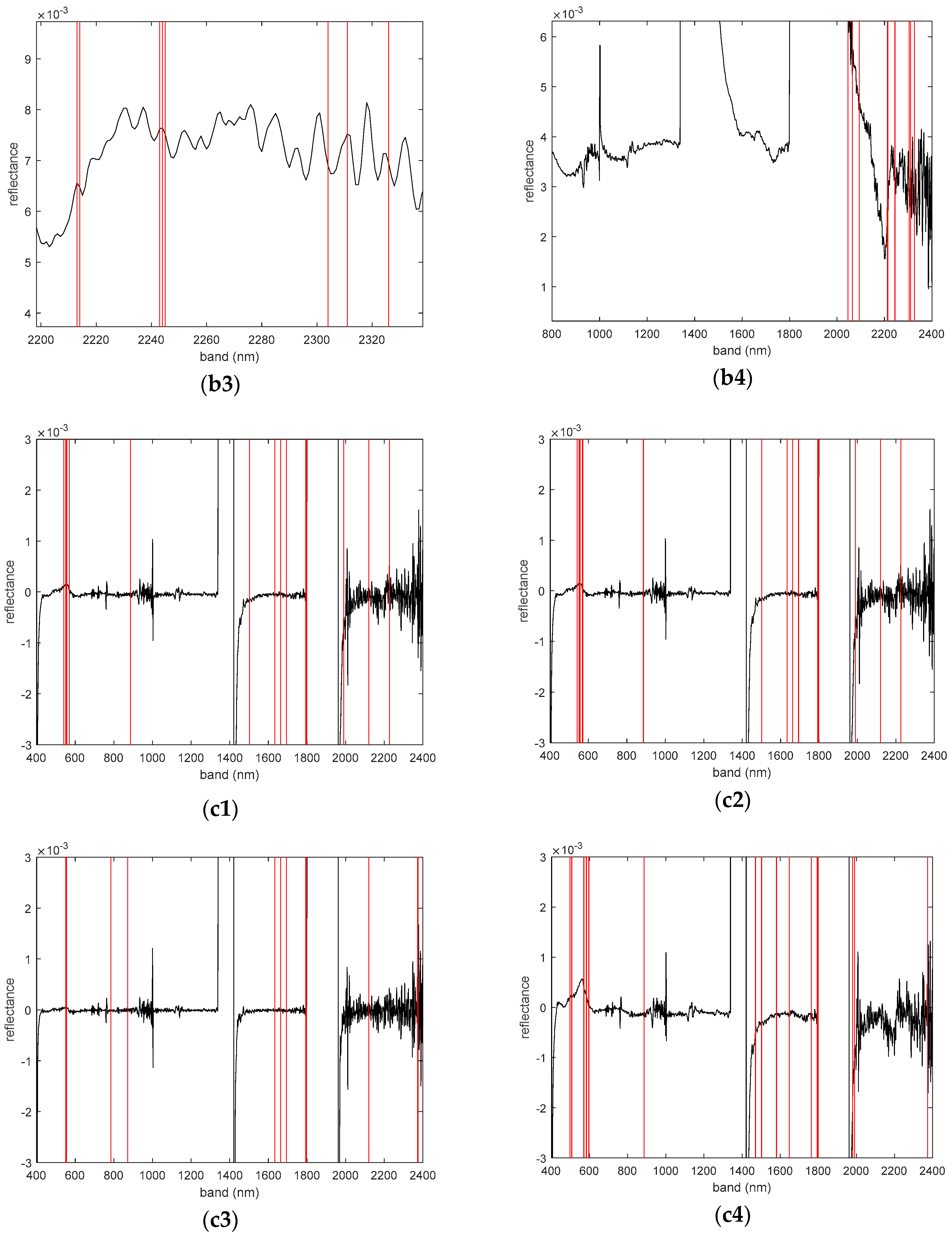
Figure 9.
Results of best R-FOD-CC1-CARS-GRNN model: (a1) validation result of I Zone and (a2) feature bands of I Zone; (b1) validation result of II Zone, (b2) feature bands of II Zone; (c1) validation result of III Zone and (c2) feature bands of III Zone.
It can be seen from Figure 9a1–c1 that the samples of the GRNN model in the three zones are more concentrated near the regression line (y = x), and the R2, RMSE, and RPD of the resulting regression model are in the I, II, and III Zone are 0.7784, 1.8762, and 2.0568; 0.7912, 3.4001, and 1.8985; 0.8192, 6.6260, and 1.8190, respectively. This further shows that the CARS method can effectively estimate the wavelength variable of salinity, and the CARS-based GNN model has a higher accuracy, a higher degree of fitting, and a better predictive ability. This shows that the CARS coupled CC1 method can screen out the sensitive bands for predicting salinity, reduce the number of modeling variables, and help improve the accuracy of the model.
It can be seen from Figure 9a2–c2 that the characteristic bands of the three regions are mainly concentrated in visible light and near infrared. For example, I Zone appears around 618 nm and 1275 nm, II Zone appears around 469 nm and 744 nm, and III Zone appears around 555 nm and 872 nm.
4. Discussion
4.1. Comparison of Estimation Accuracy between Linear Model and Nonlinear Model
At present, there are few comparative studies of various machine learning models in the field of spectra, especially the field hyperspectral estimation of salinity based on fractional-order derivative. For example, Wang et al. [44] combined the fractional-order derivative and partial least square (PLS) method to estimate soil chromium, but he only used a PLS-based estimation model method, and did not compare and analyze the prediction effects of different models. Hong et al. [45] combined fractional-order derivative and two regression techniques (PLS and PLS–SVM) to predict soil organic matter content, but he did not compare and analyze the estimation effect of linear and machine learning models.
Moreover, the destruction and change of the original ecological balance of the soil caused by human activities have caused changes in soil moisture, organic matter, salinity, and other indicators. However, there are few reports and studies on the estimation of saline soil under different degrees of human disturbance in arid zones. For example.
Duan et al. [46] used multiple stepwise line regression (SMLR) to estimate the saline soil under different disturbance extent. Fu et al. [47] adopted the fractional-order derivative to process soil total phosphorus content. However, they did not analyze the comparative the estimation effect of the machine learning model and PLSR model. Although Tian et al. [48] used a chaotic system to study the degree of soil salinization classification in different regions, she had not studied the effect of this method on the estimation of salt content.
It can be seen from the previous simulation results that the estimation accuracy of the prediction model based on the R-FOD-CC1 method is higher than that based on the R-FOD-CC5 method. Meanwhile, the GRNN-based machine learning model has the best effect in estimating the soil salt content in II and III Zone, while the machine learning model based on ELM and RF has poor effect in predicting the soil salt content in I, II, and III Zone. This is because GRNN is a radial basis function network based on mathematical statistics, which has stronger advantages than traditional neural networks in terms of approximation ability and learning speed, and the network finally converges to an optimized regression surface with a large accumulation of samples, and has strong predictive ability when the sample data is small, so GRNN has been widely used in various fields, Such as, Xu et al. [49] used GRNN model to estimate the heavy metal under indoor spectral environment. However, GRNN currently has fewer applications for outdoor hyperspectral in saline soil.
From the division of research areas in Section 2.2, it can be seen that the soils in II and III Zones are more disturbed by human activities to a certain extent, and the changes in soil properties are more complex than in I Zone, so the nonlinear relationship between the hyperspectral reflectance of the total salt content of the soil in the II and III Zones is more obvious than that in the I Zone. Therefore, GRNN is widely used to solve data fitting problems under small sample data size and nonlinear conditions due to its powerful fitting ability. Therefore, the optimal models for predicting soil salt content in II and III Zone are all based on machine learning established by GRNN, namely R-FOD-CC1-GRNN.
In addition, for the soil in I Zone, because the soil ground surface basically maintains the original style and the vegetation coverage is relatively high, black biological crusts are common on the soil surface in I Zone due to less human disturbance, the soil properties have not changed much, the linear relationship between the hyperspectral reflectance of the soil and the total salt content in the I Zone is more obvious than that in the II and III Zones. Meanwhile, as a linear prediction model, PLSR shows good prediction performance in terms of the prediction effect of soil element content. For example, Yin et al. [50] used PLSR to estimate the heavy metal copper, the RPD is 1.56. Nowkandeh et al. [51] adopted PLSR to estimate the soil organic matter, results showed that the PLSR could provide reasonable accuracy to predict soil organic matter in entire semi-arid region. The R-FOD-CC5-PLSR model in this study estimates the RPD value of I Zone to be 1.6595, and predicts the RPD value of II and III Zone to be between 1.8 and 2.0. Therefore, the prediction performance of the soil salinity in I Zone is average, it is good in II and III Zone. At the same time, the prediction performance of R-FOD-CC1-PLSR in predicting soil salinity in I and III Zone is also good. It can be seen that the combined method of fractional-order derivative and PLSR in the study can better predict the soil salt content of each area, and the results of these studies are the same as those of scientists [52,53,54,55].
4.2. Comparison of Model Estimation Results Based on Different Characteristic Band Methods
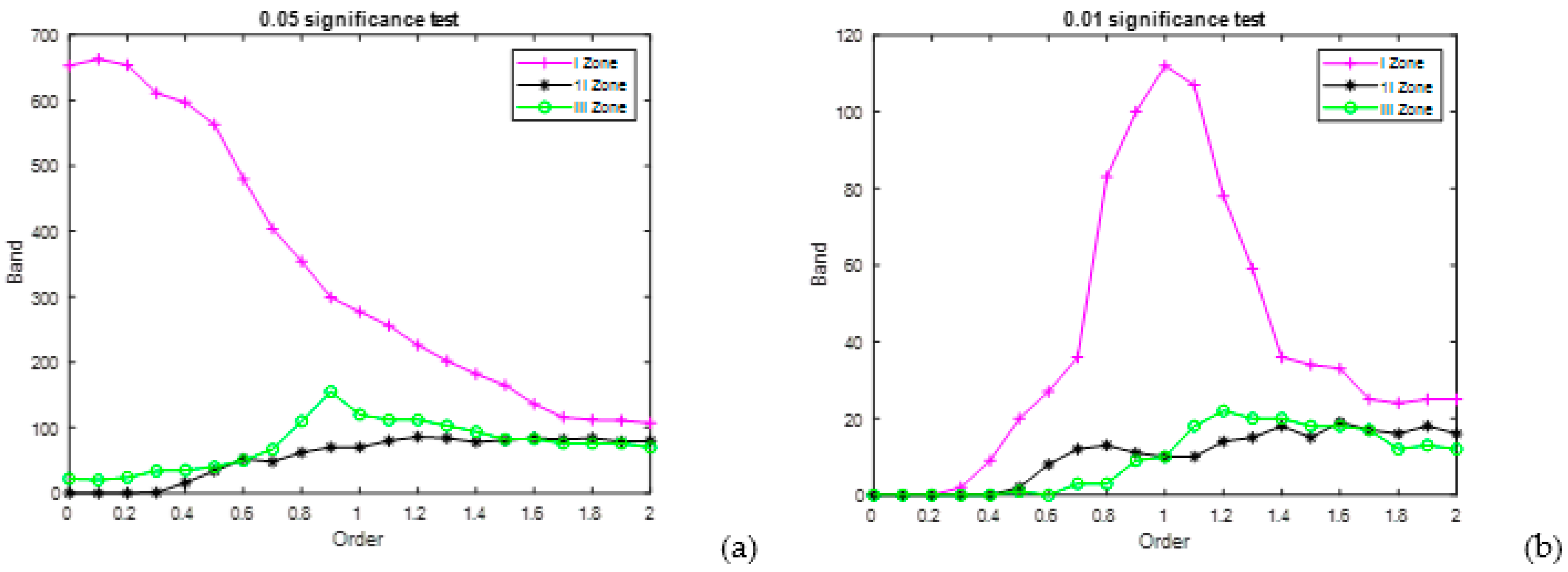
The optimization of spectral variables is necessary for soil hyperspectral analysis, which can not only reduce the complexity of the prediction model, but also remove low-correlation band variables. It is a key link to improve modeling accuracy. However, the modeling accuracy of different characteristic band selection methods is different. The number of characteristic band variables extracted by the three different methods (R-FOD-FULL, R-FOD-CC5, and R-FOD-CC1) in different research zones is quite different. Since the R-FOD-FULL method uses full band variables, there are 1759 band variables in each fractional-order, so it is not shown in the Figure. Figure 10 shows the number of characteristic band variables extracted based on different methods in each zone. Among them, R-FOD-CC5 represents the band variable that passed the 0.05 significance level test in different FOD, and R-FOD-CC1 represents the band variable that passed the 0.01 significance level test in different FOD. Figure 10a reflects that the number of characteristic band variables extracted by the R-FOD-CC5 method shows a gradual decrease trend in 1 Zone as a whole, while the change trend in II Zone and III Zone increases first and then decreases. Figure 10b reflects that the overall change trend of the number of characteristic band variables selected by the R-FOD-CC1 method in each zone is increased first and then decreased.

Figure 10.
Number of characteristic band variables extracted based on different methods:(a) 0.05 significance test; (b) 0.01 significance test.
It can also be seen in Figure 10 that when compared with the R-FOD-CC5 method, the R-FOD-CC1 method extracts fewer band variables, which are concentrated between 0.9-order and 2.0-order. Meanwhile, the average number of band variables extracted by the R-FOD-CC1 method is 50, 15, and 17 in the I, II, and III Zones, respectively. While the number of band variables selected by the R-FOD-CC5 method is about 500 between 0.0-order and 1.0-order in I Zone, and about 100 between 1.0-order and 2.0-order; and there are also about 60 in II Zone and about 80 in III Zone, respectively. The phenomenon shows that the feature band variables extracted by R-FOD-CC5 are highly redundant, which ultimately affects the prediction effect of the estimation model, resulting in low prediction accuracy and large amount of calculation. However, the characteristic band variables extracted by R-FOD-CC1 are less, especially in the II and III Zones less than 20, and the redundancy between the bands is very small. Therefore, the estimation accuracy of the prediction model based on the R-FOD-CC1 method is higher than that based on the R-FOD-CC5 method.
In the past, many scholars used correlation analysis to study the relationship between salinity and soil spectral reflectance, and the band with high correlation coefficient was regarded as the sensitive band of salinity. For example, Zhang et al. [56] adopted all the bands passed the significance test at the level of 0.01 as features to participate in the modelling process, and the estimation effect of predicting soil salt content by using PLSR modeling was very good. Chen et al. [57] used the wavelengths which passed the 0.01 significant test of correlation coefficient as the input feature. These indicate that the method of extracting characteristic band variables based on the significance level is feasible, but there are few previous studies on the comparative analysis of soil salt content based on machine learning models and PLSR model in combination with 0.01 and 0.05 significance levels.
Now more and more scholars use the CARS variable optimization method to screen the characteristic variables of the original spectrum, filter out invalid variables or redundant variables from the full band, and, finally, select the sensitive band. For example, Bao et al. [58] used CARS algorithm to screen the optimal variable subset of soil organic matter using four soil types: black soil, chernozem, aeolian soil, and meadow soil, and the sensitive band was concentrated in the range of 1350–2400 nm. Xu et al. [59] used ASD spectroscopy to determine the density of rice root by SVM model, and CARS method was been selected to obtain spectral feature variables, simulation results showed that CARS-SVM model had good predictive performance. Huang et al. [60] used near-infrared spectroscopy to measure tobacco samples, the model combined with CARS and PLSR was positive for Zn, Cd, As, Cr, Hg, and Pb, experimental results showed that those method could obtain heavy metal content.
CC and CARS are commonly used methods to select spectral variables. The CARS algorithm selects the band points with the larger absolute value of the regression coefficient in the PLSR model, which can effectively select the optimal band combination related to the soil salinity properties. The combination of CARS and CC1 can better screen out the optimal subset of variables. The research results of this paper are basically consistent with those of scientists. Therefore, the hyperspectral characteristic band variable screening method can eliminate more irrelevant information in the spectral signal, eliminate the collinearity existing between the variables, and simplify and improve the accuracy of the prediction model. Both CC1 and CARS methods are suitable for the selection of high-dimensional data variables of the spectrum.
5. Conclusions
When the original soil spectrum is processed by fractional-order derivative, the spectral curve shows a great change, the subtle spectral information is gradually amplified, and the spectral sensitivity is also improved to a certain extent. The results of this study fully demonstrate that the method based on R-FOD-CC1-CARS has better effects, which has a good promotion effect on the identification, and the elimination of redundant information, it also can greatly simplify the computational complexity. Meanwhile, it can see from the simulation results of the four machine prediction models (GRNN, ELM, RF, and PLSR) that the GRNN model has the best estimation effect, followed by the PLSR model, and the RF model has the worst estimation effect. The best model for the three Zones is also R-FOD-CC1-CARS-GRNN, and the RPD values is 2.0568, 1.8985, and 1.8190, respectively, its estimation performance is great, fine, and fine. Therefore, this study uses the CC1-CARS coupling algorithm to improve the accuracy of salt prediction, indicating that the CC1-CARS coupling algorithm is an effective band selection method for soil spectral analysis.
Author Contributions
Methodology, C.F. and A.T.; software, C.F.; experiment, A.T. and H.X.; validation, A.T. and J.Z.; formal analysis, D.Z. and J.Z.; writing the original manuscript, C.F.; reviewing and editing the manuscript, A.T.; funding acquisition, H.X., A.T., C.F., and J.Z. All authors have read and agreed to the published version of the manuscript.
Funding
The authors would like to thank the National Natural Science Foundation of China under 41901065, 41671198, 42067029, 41761081, 41761041. Key Project of Local Undergraduate Universities of Yunnan Provincial Department of Science and Technology under 2019FH001(-005).
Institutional Review Board Statement
Not applicable.
Informed Consent Statement
Not applicable.
Data Availability Statement
Not applicable.
Acknowledgments
We would like to thank the chemical analysis results of soil salt contents by Xinjiang Institute of Ecology and Geography.
Conflicts of Interest
The authors declared that there are no conflict of interest to this paper.
References
- Ding, J.; Yang, S.; Shi, Q.; Wei, Y.; Wang, F. Using Apparent Electrical Conductivity as Indicator for Investigating Potential Spatial Variation of Soil Salinity across Seven Oases along Tarim River in Southern Xinjiang, China. Remote Sens. 2020, 12, 2601. [Google Scholar] [CrossRef]
- Wang, J.; Ding, J.; Yu, D.; Teng, D.; He, B.; Chen, X.; Ge, X.; Zhang, Z.; Wang, Y.; Yang, X.; et al. Machine learning-based detection of soil salinity in an arid desert region, Northwest China: A comparison between Landsat-8 OLI and Sentinel-2 MSI. Sci. Total Environ. 2020, 707, 136092. [Google Scholar] [CrossRef] [PubMed]
- Tian, A.; Fu, C.; Yao, H.; Su, X.; Xiong, H. A New Methodology of Soil Salinization Degree Classification by Probability Neural Network Model based on Centroid of Fractional Lorenz Chaos Self-Synchronization Error Dynamics. IEEE Trans. Geosci. Remote Sens. 2020, 58, 799–810. [Google Scholar] [CrossRef]
- Yang, X.; Yu, Y. Estimating soil salinity under various moisture conditions: An experimental study. IEEE Trans. Geosci. Remote Sens. 2017, 55, 2525–2533. [Google Scholar] [CrossRef]
- Nawar, S.; Munnaf, M.A.; Mouazen, A.M. Machine Learning Based On-Line Prediction of Soil Organic Carbon after Removal of Soil Moisture Effect. Remote Sens. 2020, 12, 1308. [Google Scholar] [CrossRef] [Green Version]
- Xiao, D.; Vu, Q.H.; Le, B.T. Salt content in saline-alkali soil detection using visible-near infrared spectroscopy and a 2D deep learning. Microchem. J. 2021, 165, 106182. [Google Scholar] [CrossRef]
- Xu, H.; Xu, D.; Chen, S.; Ma, W.; Shi, Z. Rapid Determination of Soil Class Based on Visible-Near Infrared, Mid-Infrared Spectroscopy and Data Fusion. Remote Sens. 2020, 12, 1512. [Google Scholar] [CrossRef]
- Askari, M.S.; O’Rourke, S.M.; Holden, N.M. A comparison of point and imaging visible-near infrared spectroscopy for determining soil organic carbon. J. Near Infrared Spectrosc. 2018, 26, 133–146. [Google Scholar] [CrossRef]
- Shen, L.; Gao, M.; Yan, J.; Li, Z.; Leng, P.; Duan, Q.Y. Hyperspectral Estimation of Soil Organic Matter Content using Different Spectral Preprocessing Techniques and PLSR Method. Remote Sens. 2020, 12, 1206. [Google Scholar] [CrossRef] [Green Version]
- Wang, L.; Zhang, B.; Shen, Q.; Yao, Y.; Zhang, S.; Wei, H.; Yao, R.; Zhang, Y. Estimation of Soil Salt and Ion Contents Based on Hyperspectral Remote Sensing Data: A Case Study of Baidunzi Basin, China. Water 2021, 13, 559. [Google Scholar] [CrossRef]
- Kahaer, Y.; Tashpolat, N.; Shi, Q.; Liu, S. Possibility of Zhuhai-1 Hyperspectral Imagery for Monitoring Salinized Soil Moisture Content Using Fractional Order Differentially Optimized Spectral Indices. Water 2020, 12, 3360. [Google Scholar] [CrossRef]
- An, D.; Zhao, G.; Chang, C.; Wang, Z.; Li, P.; Zhang, T.; Jia, J. Hyperspectral field estimation and remote-sensing inversion of salt content in coastal saline soils of the Yellow River Delta. Int. J. Remote Sens. 2016, 37, 455–470. [Google Scholar] [CrossRef]
- Wang, X.; Zhang, F.; Ding, J.; Kung, H.; Latif, A.; Johnson, V.C. Estimation of soil salt content (SSC) in the Ebinur LakeWetland National Nature Reserve (ELWNNR), Northwest China, based on a Bootstrap-BP neural network model and optimal spectral indices. Sci. Total Environ. 2018, 615, 918–930. [Google Scholar] [CrossRef] [PubMed]
- Ben-Dor, E.; Granot, A.; Notesco, G. A simple apparatus to measure soil spectral information in the field under stable conditions. Geoderma 2017, 306, 73–80. [Google Scholar] [CrossRef]
- Tang, Y.; Chen, Z. Soil pH Prediction Based on Convelution Neural Network and Near Infrared Spectrpscopy. Spectrosc. Spectr. Anal. 2021, 41, 892–897. [Google Scholar]
- Yuan, Z.; Wei, L.; Zhang, Y.; Yu, M.; Yan, X. Hyperspectral Inversion and Analysis of Heavy Metal Arsenic Content in Farmland Soil Based on Optimizing CARS Combined with PSO-SVM Algorithm. Spectrosc. Spectr. Anal. 2020, 40, 567–573. [Google Scholar]
- Sourav, B.; Vasit, S.; Maitiniyazi, M.; Matthew, M.; Maria, N.; Nadia, S.; Todd, C.M. Quantifying Leaf Chlorophyll Concentration of Sorghum from Hyperspectral Data Using Derivative Calculus and Machine Learning. Remote Sens. 2020, 12, 2082. [Google Scholar]
- Meng, X.; Bao, Y.; Ye, Q.; Liu, H.; Zhang, X.; Tang, H.; Zhang, X. Soil Organic Matter Prediction Model with Satellite Hyperspectral Image Based on Optimized Denoising Method. Remote Sens. 2021, 13, 2273. [Google Scholar] [CrossRef]
- Wang, Z.; Zhang, X.; Zhang, F.; Chan, N.; Kunge, H.; Liu, S.; Deng, L. Estimation of soil salt content using machine learning techniques based on remote-sensing fractional derivatives, a case study in the Ebinur Lake Wetland National Nature Reserve, Northwest China. Ecol. Indic. 2020, 119, 106869. [Google Scholar] [CrossRef]
- Chen, L.; Lai, J.; Tan, K.; Wang, X.; Chen, Y.; Ding, J. Development of a soil heavy metal estimation method based on a spectral index: Combining fractional-order derivative pretreatment and the absorption mechanism. Sci. Total Environ. 2021, 11, 151882. [Google Scholar] [CrossRef]
- Abulaiti, Y.; Sawut, M.; Maimaitiaili, B.; Chunyue, M. A possible fractional order derivative and optimized spectral indices for assessing total nitrogen content in cotton. Comput. Electron. Agric. 2020, 171, 105275. [Google Scholar] [CrossRef]
- Hong, Y.; Liua, Y.; Chen, Y.; Liu, Y.; Yu, L.; Liu, Y.; Cheng, H. Application of fractional-order derivative in the quantitative estimation of soil organic matter content through visible and near-infrared spectroscopy. Geoderma 2019, 337, 758–769. [Google Scholar] [CrossRef]
- Zhang, B.; Li, W.; Li, X.; See-Kiong, N. Intelligent Fault Diagnosis Under Varying Working Conditions Based on Domain Adaptive Convolutional Neural Networks. IEEE Access 2018, 6, 66367–66384. [Google Scholar] [CrossRef]
- Chen, Z.; Yang, Y.; Jiang, C.; Hao, J.; Zhang, L. Light Sensor Based Occupancy Estimation via Bayes Filter With Neural Networks. IEEE Trans. Ind. Electron. 2020, 67, 5787–5797. [Google Scholar] [CrossRef]
- Tian, A.; Zhao, J.; Tang, B.; Zhu, D.; Fu, C.; Xiong, H. Hyperspectral Prediction of Soil Total Salt Content by Different Disturbance Degree under a Fractional-Order Differential Model with Differing Spectral Transformations. Remote Sens. 2021, 13, 4283. [Google Scholar] [CrossRef]
- Tian, A.; Zhao, J.; Tang, B.; Zhu, D.; Fu, C.; Xiong, H. Study on the Pretreatment of Soil Hyperspectral and Na+ Ion Data under Different Degrees of Human Activity Stress by Fractional-Order Derivatives. Remote Sens. 2021, 13, 3974. [Google Scholar] [CrossRef]
- Pano-Azucena, A.D.; Ovilla-Martinez, B.; Tlelo-Cuautle, E.; Muñoz-Pacheco, J.M.; la Fraga, L.G. FPGA-based implementation of different families of fractional-order chaotic oscillators applying Grünwald–Letnikov method. Commun. Nonlinear Sci. Numer. Simul. 2019, 72, 516–527. [Google Scholar] [CrossRef]
- Chen, H.; Holland, F.; Stynes, M. An analysis of the Grünwald–Letnikov scheme for initial-value problems with weakly singular solutions. Appl. Numer. Math. 2019, 139, 52–61. [Google Scholar] [CrossRef]
- Sadeghi, F.; Yu, Y.; Zhu, X.; Li, J. Damage identification of steel-concrete composite beams based on modal strain energy changes through general regression neural network. Eng. Struct. 2021, 244, 112824. [Google Scholar] [CrossRef]
- Mirzaei, S.; Moradi, S.; Ehzari, H.; Farhadian, N.; Shahlaei, M. Application of general regression neural network and central composite design in fabrication and performance of magnetite (Fe3O4) modified carbon paste electrode for the electrochemical detection of Clomiphene. Microchem. J. 2019, 147, 1028–1037. [Google Scholar] [CrossRef]
- Tian, X.; Jiao, W.; Liu, T.; Ren, L.; Song, B. Leakage detection of low-pressure gas distribution pipeline system based on linear fitting and extreme learning machine. Int. J. Press. Vessel. Pip. 2021, 194, 104553. [Google Scholar] [CrossRef]
- Duan, M.; Li, K.L.; Liao, X.; Li, K.Q. A Parallel Multiclassification Algorithm for Big Data Using an Extreme Learning Machine. IEEE Trans. Neural Netw. Learn. Syst. 2018, 29, 2337–2351. [Google Scholar] [CrossRef] [PubMed]
- Shah, S.H.; Angel, Y.; Houborg, R.; Ali, S.; McCabe, M.F. A Random Forest Machine Learning Approach for the Retrieval of Leaf Chlorophyll Content in Wheat. Remote Sens. 2019, 11, 920. [Google Scholar] [CrossRef] [Green Version]
- Sun, J.; Yang, W.; Zhang, M.; Feng, M.; Xiao, L.; Ding, G. Estimation of water content in corn leaves using hyperspectral data based on fractional order Savitzky-Golay derivation coupled with wavelength selection. Comput. Electron. Agric. 2021, 182, 05989. [Google Scholar] [CrossRef]
- Biney, J.K.M.; Borůvka, L.; Agyeman, P.C.; Němeček, K.; Klement, A. Comparison of Field and Laboratory Wet Soil Spectra in the Vis-NIR Range for Soil Organic Carbon Prediction in the Absence of Laboratory Dry Measurements. Remote Sens. 2020, 12, 3082. [Google Scholar] [CrossRef]
- Guo, P.; Li, M.; Luo, W.; Cha, Z. Estimation of foliar nitrogen of rubber trees using hyperspectral reflectance with feature bands. Infrared Phys. Technol. 2019, 102, 103021. [Google Scholar] [CrossRef]
- Gao, L.; Zhu, X.; Han, Z.; Wang, L.; Zhao, G.; Jiang, Y. Spectroscopy-Based Soil Organic Matter Estimation in Brown Forest Soil Areas of the Shandong Peninsula, China. Pedosphere 2019, 29, 810–818. [Google Scholar] [CrossRef]
- Li, Q.; Xie, J.; Zhang, J.; Yan, H.; Xiong, Y.; Liu, W.; Min, S. A global model for the determination of prohibited addition in pesticide formulations by near infrared spectroscopy. Infrared Phys. Technol. 2020, 105, 103191. [Google Scholar] [CrossRef]
- Xing, Z.; Du, C.; Shen, Y.; Ma, F.; Zhou, J. A method combining FTIR-ATR and Raman spectroscopy to determine soil organic matter: Improvement of prediction accuracy using competitive adaptive reweighted sampling (CARS). Comput. Electron. Agric. 2021, 191, 106549. [Google Scholar] [CrossRef]
- Kumar, K. Competitive adaptive reweighted sampling assisted partial least square analysis of excitation-emission matrix fluorescence spectroscopic data sets of certain polycyclic aromatic hydrocarbons. Spectrochim. Acta Part A Mol. Biomol. Spectrosc. 2021, 244, 118874. [Google Scholar] [CrossRef]
- Peng, J.; Biswas, A.; Jiang, Q.; Zhao, R.; Hu, J.; Hu, B.; Shi, Z. Estimating soil salinity from remote sensing and terrain data in southern Xinjiang Province, China. Geoderma 2019, 337, 1309–1319. [Google Scholar] [CrossRef]
- Cezar, E.; Nanni, M.R.; Crusiol, L.G.T.; Sun, L.; Chicati, M.S.; Furlanetto, R.H.; Rodrigues, M.; Sibaldelli, R.N.R.; Silva, G.F.C.; de Oliveira, K.M.; et al. Strategies for the Development of Spectral Models for Soil Organic Matter Estimation. Remote Sens. 2021, 13, 1376. [Google Scholar] [CrossRef]
- Wang, N.; Xue, J.; Peng, J.; Biswas, A.; He, Y.; Shi, Z. Integrating Remote Sensing and Landscape Characteristics to Estimate Soil Salinity Using Machine Learning Methods: A Case Study from Southern Xinjiang, China. Remote Sens. 2020, 12, 4118. [Google Scholar] [CrossRef]
- Wang, J.; Hu, X.; Shi, T.; He, L.; Hu, W.; Wu, G. Assessing toxic metal chromium in the soil in coal mining areas via proximal sensing: Prerequisites for land rehabilitation and sustainable development. Geoderma 2021, 405, 115399. [Google Scholar] [CrossRef]
- Hong, Y.; Chen, S.; Liu, Y.; Zhang, Y.; Yu, L.; Chen, Y.; Liu, Y.; Cheng, H.; Liu, L. Combination of fractional order derivative and memory-based learning algorithm to improve the estimation accuracy of soil organic matter by visible and near-infrared spectroscopy. Catena 2019, 174, 104–116. [Google Scholar] [CrossRef]
- Duan, P.; Xiong, H.; Li, R.; Zhang, L. A quantitative analysis of the reflectance of the saline soil under different disturbance extent. Sepctrosc. Spectr. Anal. 2017, 37, 571–576. [Google Scholar]
- Fu, C.; Gan, S.; Yuan, X.; Xiong, H.; Tian, A. Pretreatment of Total Phosphorus Content in Saline Soil in Arid Area by Fractional Differential Algorithm. Sens. Mater. 2018, 30, 2469–2477. [Google Scholar] [CrossRef]
- Tian, A.; Fu, C.; Xiong, H.; Yau, H.-T. Innovative Intelligent Methodology for the Classification of Soil Salinization Degree Using a Fractional-Order Master-Slave Chaotic System. Int. J. Bifurc. Chaos 2019, 29, 1950026. [Google Scholar] [CrossRef]
- Xu, X.; Chen, S.; Ren, L.; Han, C.; Lv, D.; Zhang, Y.; Ai, F. Estimation of Heavy Metals in Agricultural Soils Using Vis-NIR Spectroscopy with Fractional-Order Derivative and Generalized Regression Neural Network. Remote Sens. 2021, 13, 2718. [Google Scholar] [CrossRef]
- Yin, F.; Wu, M.; Liu, L.; Zhu, Y.; Feng, J.; Yin, D.; Yin, C.; Yin, C. Predicting the abundance of copper in soil using reflectance spectroscopy and GF5 hyperspectral imagery. Int. J. Appl. Earth Obs. Geoinf. 2021, 102, 102420. [Google Scholar] [CrossRef]
- Nowkandeh, S.M.; Noroozi, A.A.; Homaeec, M. Estimating soil organic matter content from Hyperion reflectance images using PLSR, PCR, MinR and SWR models in semi-arid regions of Iran. Environ. Dev. 2018, 25, 23–32. [Google Scholar] [CrossRef]
- Hong, Y.; Shen, R.; Cheng, H.; Chen, Y.; Zhang, Y.; Liu, Y.; Zhou, M.; Yu, L.; Liu, Y.; Liu, Y. Estimating lead and zinc concentrations in peri-urban agricultural soils through reflectance spectroscopy: Effects of fractional-order derivative and random forest. Sci. Total Environ. 2019, 651, 1969–1982. [Google Scholar] [CrossRef]
- Wang, J.; Ding, J.; Abulimiti, A.; Cai, L. Quantitative estimation of soil salinity by means of different modeling methods and visible-near infrared (VIS-NIR) spectroscopy, Ebinur Lake Wetland, Northwest China. PeerJ 2018, 6, e4703. [Google Scholar] [CrossRef] [Green Version]
- Lao, C.; Chen, J.; Zhang, Z.; Chen, Y.; Ma, Y.; Chen, H.; Gu, X.; Ning, J.; Jin, J.; Li, X. Predicting the contents of soil salt and major water-soluble ions with fractional-order derivative spectral indices and variable selection. Comput. Electron. Agric. 2021, 182, 106031. [Google Scholar] [CrossRef]
- Zhang, Z.; Ding, J.; Wang, J.; Ge, X. Prediction of soil organic matter in northwestern China using fractional order derivative spectroscopy and modified normalized difference indices. Catena 2020, 185, 104257. [Google Scholar] [CrossRef]
- Zhang, D.; Tiyip, T.; Ding, J.; Zhang, F.; Nurmemet, I.; Kelimu, A.; Wang, J. Quantitative Estimating Salt Content of Saline Soil Using Laboratory Hyperspectral Data Treated by Fractional Derivative. J. Spectrosc. 2016, 2016, 1081674. [Google Scholar] [CrossRef]
- Chen, K.; Li, C.; Tang, R. Estimation of the nitrogen concentration of rubber tree using fractional calculus augmented NIR spectra. Ind. Crops Prod. 2017, 108, 831–839. [Google Scholar] [CrossRef]
- Bao, Y.; Meng, X.; Ustin, S.; Wang, X.; Zhang, X.; Liu, H.; Tang, H. Vis-SWIR spectral prediction model for soil organic matter with different grouping strategies. Catena 2020, 195, 104703. [Google Scholar] [CrossRef]
- Xu, S.; Zhao, Y.; Wang, M.; Shi, X. Determination of rice root density from Vis–NIR spectroscopy by support vector machine regression and spectral variable selection techniques. Catena 2017, 157, 12–23. [Google Scholar] [CrossRef]
- Huang, Y.; Du, G.; Ma, Y.; Zhou, J. Predicting heavy metals in dark sun-cured tobacco by near-infrared spectroscopy modeling based on the optimized variable selections. Ind. Crops Prod. 2021, 172, 114003. [Google Scholar] [CrossRef]

Publisher’s Note: MDPI stays neutral with regard to jurisdictional claims in published maps and institutional affiliations. |
© 2021 by the authors. Licensee MDPI, Basel, Switzerland. This article is an open access article distributed under the terms and conditions of the Creative Commons Attribution (CC BY) license (https://creativecommons.org/licenses/by/4.0/).