Coarse-to-Fine Image Registration for Multi-Temporal High Resolution Remote Sensing Based on a Low-Rank Constraint

Abstract

For multi-temporal high resolution remote sensing images, the image registration is important but difficult due to the high resolution and low-stability land-cover. Especially, the changing of land-cover, solar altitude angle, radiation intensity, and terrain fluctuation distortion in the overlapping areas can represent different image characteristics. These time-varying properties cause traditional registration methods with known reference information to fault. Therefore, in this paper we propose a comprehensive coarse-to-fine registration (CCFR) algorithm. First, we design a low-rank constraint-based batch reference extraction (LRC-BRE) method. Under the low-rank constraint, the stable features with highly spatial co-occurrence can be reconstructed via matrix decomposition, and are set as reference images to batch registration. Second, we improve the general feature registration with block feature matching and local linear transformation (BFM-LLT) operators including match outlier filtering (MOF) on regional mutual information and dual-weighted block fitting (DWBF). Finally, based on combining LRC-BRE and BFM-LLT, CCFR is integrated. Experimental results show that the proposed method has a good batch alignment effect, especially in the registration of large difference image pairs. The proposed CCFR achieves a significant performance improvement over many state-of-the-art registration algorithms.

1. Introduction

Multi-temporal remote sensing image registration is a key preprocessing step for remote sensing image fusion [1,2], change detection [3,4], super-resolution reconstruction [5], and collaborative analysis [6]. In recent years, remote sensing image registration has mostly focused on solving the effects of radiation differences and geometric distortions by constructing robust feature descriptors [7,8], better screening of mismatched features [9,10], integrating multiple methods [11,12], and so on. Although research on multi-temporal image registration in complex terrain areas has been conducted [13,14], there are few studies devoted to accurate registration in complex terrain areas with low-stability land-cover. The low stability of features mentioned in this paper mainly refers to the land-cover changes caused by seasonal rotation, geological alteration, human activities, and other factors, which lead to huge imaging differences of the same plot in different time series. Common low-stability features include mining, cultivated farmland, and seasonal deciduous woody vegetation under high resolution imaging conditions. Complex terrain mainly refers to undulating mountains and large-scale artificial elevation features (such as dams and buildings) under high resolution conditions. For multi-temporal remote sensing images, radiation differences including the difference of radiation intensity and the change of solar altitude angle are also an important factor leading to differences in ground object imaging; in particular, changes of solar altitude angles lead to different degrees of shadow occlusion and contour diversity of mountainous and elevation ground objects. In addition, differences of shooting inclinations lead to complex geometric deformations of mountainous and elevation ground objects. Mountainous areas with different seasonal vegetation coverage, irregular mining, and beneficiation activities are typical representatives of low-stability and complex terrain, as shown in Figure 1. Due to the mixed influence of the above multiple factors, the remote sensing images have different period features in terms of gray, texture, and contour features, which bring challenges to the accurate temporal registration.

Currently, remote sensing images are registered based on the geocoding generated by satellite orbit parameters [15]. Affected by the accuracy of satellite positioning and control, these technologies can largely eliminate the global geometric distortion but generate images with ten to dozens of pixel offsets. For mountainous areas with complex terrain, in order to improve the registration accuracy based on geocoding, it is necessary to correct the image point element offset caused by terrain fluctuation with the help of a high-precision digital elevation model (DEM) [16] and a reference image map corrected by ground control points. Limited by the accuracy of the available DEM and the lack of reference images corrected by sufficient ground control points, there are still different degrees of alignment errors in local areas with serious distortion in mountainous areas after ortho-rectification [17,18]. For higher image alignment accuracy, it is necessary to further correct with the help of an automatic image registration method. In addition, the low-stability surface makes it difficult to automatically match the control points between the sensed image and the reference image, in which accurate manual auxiliary matching is also a challenging work.

The performance of an image registration algorithm depends on its image matching step and the transformation function. Common image matching drivers include intensity matching, feature matching, density matching, and other similarity matching algorithms. According to different domains of transformation, spatial transformation estimation methods include global mapping models, local mapping models, and elastic registration [19,20].

The intensity-based method usually uses the gray information of the image to measure the similarity and realize the global spatial transformation in the area. Based on statistical correlation such as normalized cross correlation (NCC) [21,22], mutual information (MI) [23,24] has a high applicability for remote sensing image registration without prominent detail features, but it is unable to deal with complex area deformation. In order to solve the registration of large-scale geometric deformation and complex terrain, most of the relevant studies focus on the combination of regional intensity similarity and local features. Usually, the feature-based method is used as a coarse registration to calculate parameters, which can be used as the initial condition to perform fine registration using an intensity-based method [11,25]. Some researchers improve the performance of registration by applying gradient features [26] and wavelet-like features [27] to image descriptors.

The feature-based methods separate image feature matching and spatial transformation, which can be used with a variety of local transformation modes to deal with complex deformation. SIFT [28] and its variants (SURF [29], ASIFT [30], and PCA-SIFT [31]) are widely used feature extractors. These extracted features are robust to changes in terms of brightness, rotation, and scaling. The ORB [32] and BRISK [33] algorithms belong to a corner detection method based on FAST [34], which improves the computational efficiency by using binary feature description words. In recent years, for the complex nonlinear radiation intensity difference between multimodal remote sensing images, feature algorithms, such as deny oriented gradient feature (DOGH) [7] and histogram of oriented phase convergence (HOPC) [35], have been proposed and achieved good experimental results in feature matching of optical and SAR image pairs. In order to solve the significant radiation difference between multi-temporal optical remote sensing images, the PSO-SIFT [8] algorithm gives a new gradient definition to each pixel in Gauss scale space to increase the robustness of the gradient direction and size difference in the same region. Aiming at the significant geometric distortion and radiation difference between multi-source optical remote sensing images, Chen et al. [10] proposed an iterative scale invariant feature transformation method to continuously improve the registration accuracy of remote sensing images. For local geometric distortion, Sedaghat and Ebadi [36] used an adaptive histogram quantization strategy to calculate feature position and gradient direction, so that they are robust to local view distortion. However, the above feature matching methods used to improve the robustness of feature matching for significant radiation difference and local geometric distortion achieve good results only in the medium–low resolution multisource remote sensing image registration, but pay less attention to the low stability of ground objects. In view of the impact of clouds, noise, and land-cover change on the accuracy of local registration, Feng et al. [12] proposed a step-by-step registration method combining feature and regional methods. In this method, the first step matching feature results are geometrically corrected by a region-based linear polynomial transformation model, but it is only robust to simple and small radiation differences.

The density-based methods use mostly optical flow estimation. Optical flow [37,38] can achieve per-pixel displacement estimation and is suitable for the accurate alignment of remote sensing images on complex terrain. However, this method has a limited ability to deal with large deformations between registered images, and is sensitive to low-stability surface noise, which causes resampled image texture distortion. Liu et al. [39] employed mesh segmentation to distribute the optical flow field of feature points to deal with complex non-rigid body deformation, so as to improve the robustness of optical flow registration. Xu et al. [40] used the optical flow field method to handle complicated non-rigid changes by matching dense SIFT features. However, when the image texture is inconsistent because of the local land-cover changing, the above method could cause local anomalies in the computed optical flow. In order to realize the high fidelity of the registered image in complex terrain areas, Feng et al. [13] added the detection and correction of abnormal displacement fields after the optical flow estimation.

For high resolution multi-temporal remote sensing images with low-stability land-cover and complex terrain (HMR-LC images), it is difficult to align the images facing severe radiation differences and complex geometric deformation by relying on a single registration method. Multi-level and combined registration methods are needed to solve the problems of this kind of remote sensing image registration. The feature method has good adaptability to large-scale rotation, displacement and deformation, and this method can be used together with the local transformation model to solve the inconsistency of local deformation in complex terrain. The above research experience in solving complex registration problems shows that the registration performance can be improved by the comprehensive application of feature method and regional intensity information, phase information, and structure information [10,11,25,40]. However, due to the comprehensive influence of land-cover changes, terrain fluctuations, mountain shadows, radiation changes, and other factors, the probability of feature matching errors for HMR-LC is high, which seriously affects the registration results. On the one hand, affected by changes of low land-cover, the texture features of unstable objects in the image pair are significantly different, and even the texture features of partially overlapping areas are completely changed. On the other hand, due to the influence of radiation differences and shooting inclination differences, there are serious geometric deformations and complex radiation differences in the local feature window of elevation objects and complex terrain imaging, which exceeds the invariance of features and the comparability of intensity information, and it is difficult to accurately express the complex geometric relationship of different positions using the surrounding feature information [41]. These greatly reduce the possibility of detecting consistent features in image pairs, resulting in the failure of the application of mainstream feature methods in the studied target image.

Different from the previous research ideas used to solve the influence of surface change, radiation difference, and complex terrain on registration, we no longer focus on improving the registration algorithm of single image pairs, but propose a batch reference extraction into a comprehensive coarse-to-fine registration (CCFR) framework. This framework not only realizes the robust registration of significantly different HMR-LC images, but also solves the problem of a lack of a reliable baseline image for registration.

The main contributions of this paper are as follows:

(1)

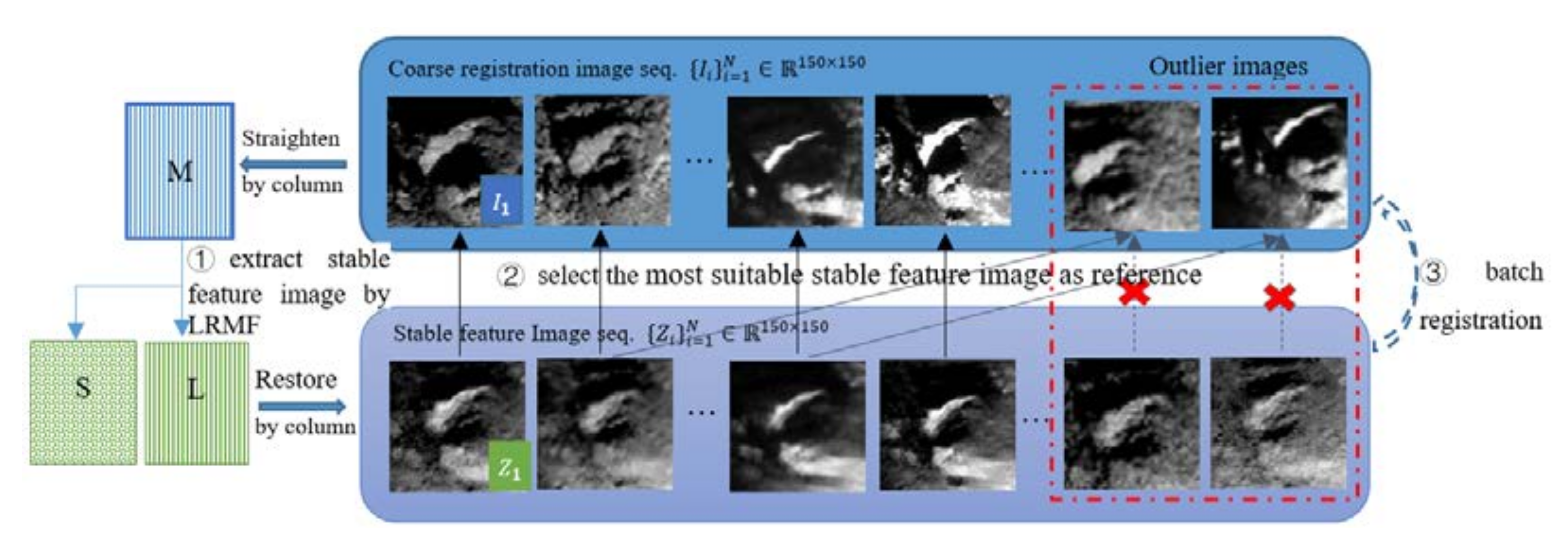
Inspired by the excellent image denoising and restoration ability of the low-rank decomposition algorithm, we design a low-rank constraint-based batch reference (LRC-BRE) method to restore the stable features holding highly spatial co-occurrence in the image sequence, and construct a corresponding batch reference, in which each original image has a respective reference.

(2)

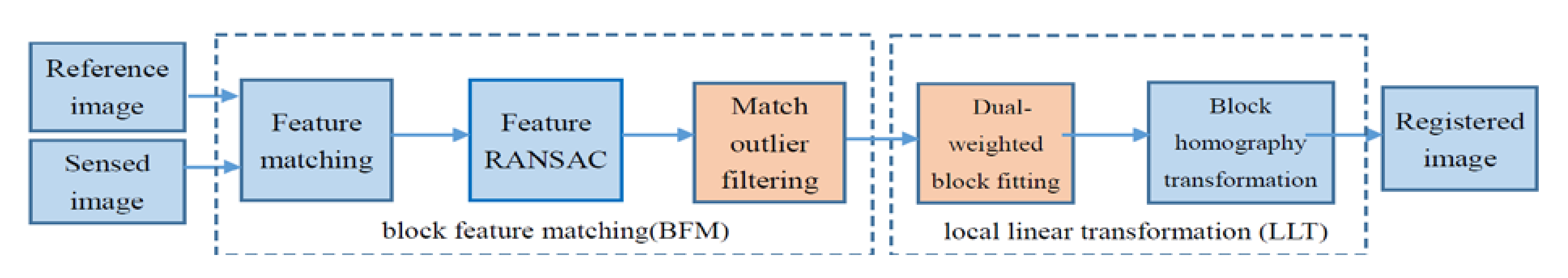
To match the original image and the reference image, the regional mutual information is considered to filter the match outliers, named as a match outlier filtering (MOF). Additionally, a dual-weighted block fitting (DWBF) is developed based on the feature inverse distance weight and feature regional similarity weight. The above two operators are integrated to form the block feature matching and local linear transformation (BFM-LLT) registration processing, which has good robustness and alignment accuracy for the coarse registration of multi-temporal remote sensing images with medium and low texture differences and for the registration of original images and stable feature images restored by LRC-BRE.

(3)

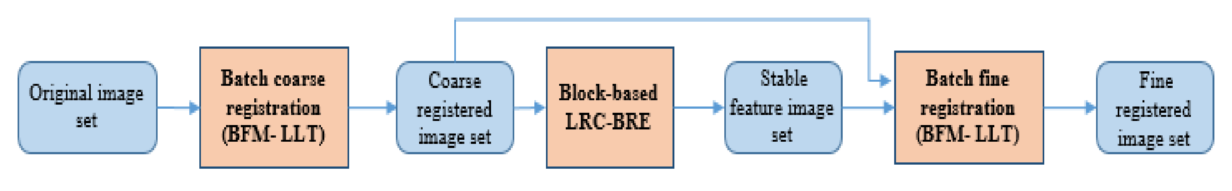
A new comprehensive coarse-to-fine registration (CCFR) framework integrated by LRC-BRE and BFM-LLT is proposed for HMR-LC images. By taking the recovered stable feature image as the reference baseline image, the proposed framework transforms the direct registration of large difference HMR-LC image pairs into the indirect registration of small and medium difference image pairs, and realizes the applicability of the mainstream image registration methods.

(4)

On GF-2 and GF-1 satellite remote sensing image datasets with low-stability land-cover and complex terrain, the experimental results show that the comprehensive registration framework CCFR is more effective than the latest registration algorithm in visual quality and quantitative evaluation, owing to the combining of LRC-BRE with good batch reference and BFM-LLT with improved alignment effect.

The rest of the paper is organized as follows: The details of the proposed method are described in Section 2. The experimental results and verification from visual and quantitative perspectives are provided in Section 3. The influencing factors of CCFR indirect registration and the work of CCFR in different optical satellite images are discussed in Section 4. Finally, our conclusions are summarized in Section 5.

2. Methods

Image feature detection and matching performance is the key step to achieve accurate image registration results. The number, accuracy and distribution of matching inner points directly affect the registration accuracy. In this section, we aim to propose a coarse-to-fine registration (CCFR) framework for multi-temporal high resolution remote sensing images, which can not only generate the stable feature reference sequence automatically, but also register the point robustly. A simple flowchart of the CCFR framework is shown in Figure 2. To solve the stable feature reference problem in batch registration processing, we introduce a low-rank constraint-based batch reference (LRC-BRE) extracting method via matrix decomposition under a low-rank constraint. In CCFR, the LRC-BRE is executed based on blocks. We also developed a block feature matching and local linear transformation (BFM-LLT) registration processing via integrating the match outlier filtering (MOF) and the dual-weighted block fitting (DWBF) operators. BFM-LLT is applicable to both batch coarse registration and batch fine registration.

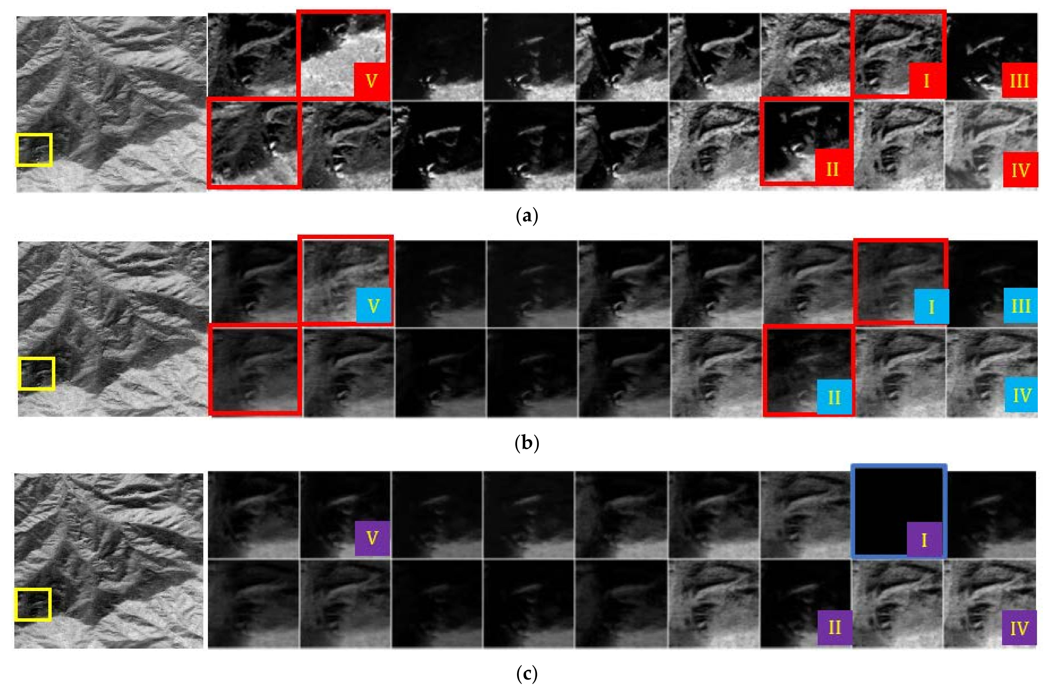
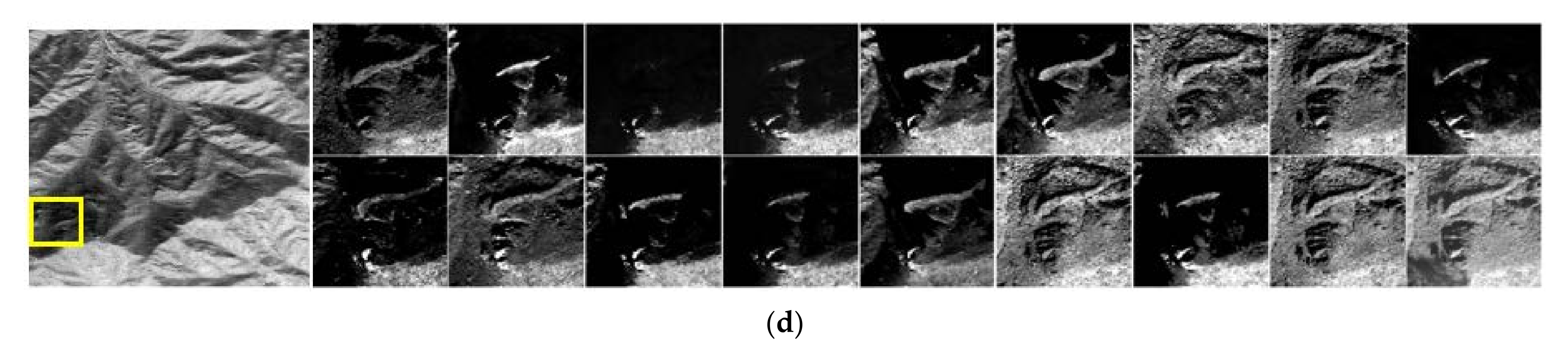
2.1. LRC-BRE: A Low-Rank Constraint-Based Batch Reference Extraction

With the rapid development of matrix rank related optimization techniques, the matrix minimum low-rank constraint attempted to replace the image similarity evaluation to realize the batch alignment of natural images [42,43]. Matrix rank correlation optimization technology originated from low-rank matrix factorization (LRMF) [44]. LRMF is an effective method of developing reliable, scalable, and robust algorithms to estimate a low-rank matrix of interest, from potentially noisy, nonlinear, and highly incomplete observations [45]. In view of the above excellent ability of LRMF, we use this model to restore the stable feature images of multi-temporal image sequences to capture a reference image with stable surface features and small radiation difference for multi-temporal remote sensing image registration. Thus, a larger number and higher accuracy of feature pairs are obtained than the direct feature detection and matching of the original image pair.

The texture difference of multi-temporal low-stability images are treated as noise, and based on the relevant hypothesis and inferences of stable feature image restoration, they can be solved from an LRMF problem. The related theorems, hypothesis and inferences are given in the appendix section.

The result of feature matching is directly related to the similarity of texture features between image pairs. The higher the texture similarity of image pairs is, the more matching features and the higher the matching accuracy can be obtained. Let ${\mathrm{diff}}_{\mathsf{\Omega }}\left({\mathit{I}}_{\mathit{i}},{\mathit{I}}_{\mathit{j}}\right)$ represent the texture difference degree of the overlapping area Ω of the locally aligned image pair $\left({\mathit{I}}_{\mathit{i}},{\mathit{I}}_{\mathit{j}}\right)$, and index ${\mathrm{diff}}_{\mathsf{\Omega }}\left({\mathit{I}}_{\mathit{i}},{\mathit{I}}_{\mathit{j}}\right)$ be the reverse index of the texture similarity of the image pair. ${\mathrm{diff}}_{\mathsf{\Omega }}\left({\mathit{I}}_{\mathit{i}},{\mathit{I}}_{\mathit{j}}\right)$ is negatively correlated with the success rate of feature matching. Let $T$ denote spatial transformation, and g(${\mathit{I}}_i^{\Omega }$) $=$ g($T\circ {\mathit{I}}_j^{\Omega }$),${\mathit{I}}_i^{\Omega }\in {\mathit{I}}_i, {\mathit{I}}_j^{\Omega }\in {\mathit{I}}_j;$ then there is ${\mathrm{diff}}_{\mathsf{\Omega }}\left({\mathit{I}}_{\mathit{i}},{\mathit{I}}_{\mathit{j}}\right)=\mathrm{diff}\left({\mathit{I}}_{\mathit{i}}^{\Omega },T\circ {\mathit{I}}_{\mathit{j}}^{\Omega }\right)$. When the image pairs $\left({\mathit{I}}_{\mathit{i}},{\mathit{I}}_{\mathit{j}}\right)$ are fully aligned, the comprehensive difference of the image pairs is equivalent to the texture difference, that is, $\mathrm{diff}\left({\mathit{I}}_{\mathit{i}},{\mathit{I}}_{\mathit{j}}\right)={\mathrm{diff}}_{\mathsf{\Omega }}\left({\mathit{I}}_{\mathit{i}},{\mathit{I}}_{\mathit{j}}\right)$; when not aligned, there is $\mathrm{diff}\left({\mathit{I}}_{\mathit{i}},{\mathit{I}}_{\mathit{j}}\right)\ge {\mathrm{diff}}_{\mathsf{\Omega }}\left({\mathit{I}}_{\mathit{i}},{\mathit{I}}_{\mathit{j}}\right)$. When there is only a local offset in the image pair, it can be considered that $\mathrm{diff}\left({\mathit{I}}_{\mathit{i}},{\mathit{I}}_{\mathit{j}}\right)\approx {\mathrm{diff}}_{\mathsf{\Omega }}\left({\mathit{I}}_{\mathit{i}},{\mathit{I}}_{\mathit{j}}\right)$. We assume that there is a threshold β. When ${\mathrm{diff}}_{\mathsf{\Omega }}\left({\mathit{I}}_{\mathit{i}},{\mathit{I}}_{\mathit{j}}\right)>\beta$, the commonly used image feature matching methods fail to obtain enough correct matching features. For high resolution multi-temporal remote sensing images with low stable surface and complex terrain, due to the comprehensive influence of ground feature changes, terrain fluctuations, mountain shadows, radiation changes, and other factors, the texture difference of some images exceeds the threshold β.

According to Inference A3 in the Appendix A, for the image sequence ${\left\{{\mathit{I}}_i\right\}}_{i=1}^N$ and its restored stable feature image sequence ${\left\{{\mathit{Z}}_i\right\}}_{i=1}^N$, the probability is $\mathrm{diff}\left({\mathit{I}}_{\mathit{i}},{\mathit{I}}_r\right)$>$\mathrm{diff}{\mathit{I}}_i,{\mathit{Z}}_i\left(1\le i\le N_{s2}\le N\right)$. According to Inference A1.1 in the Appendix A, for the image sequence ${\left\{{\mathit{I}}_i\right\}}_{i=1}^N$ conforming to Hypothesis A2 in the Appendix A and its restored stable feature image sequence ${\left\{{\mathit{Z}}_i\right\}}_{i=1}^N$, there is ${\mathit{Z}}_1\left(x,y\right)\approx \cdots \approx {\mathit{Z}}_N\left(x,y\right)$, g(${\mathit{Z}}_1$)$\approx \cdots \approx$g(${\mathit{Z}}_{\mathit{N}}$). Then, we only need to take ${\mathit{Z}}_{\mathit{i}}$ as the registration reference image and register the image pairs $\left\{{\mathit{I}}_{\mathit{i}},{\mathit{Z}}_{\mathit{i}}\right\}(1<i<N)$ one by one, which can approximately realize the registration of any image pair $\left\{{\mathit{I}}_{\mathit{i}},{\mathit{I}}_{\mathit{j}}\right\}(1<i,j<N)$ in the sequence ${\left\{{\mathit{I}}_{\mathit{i}}\right\}}_{i=1}^N$. Let ${\mathit{I}}_{\mathit{i}}^{\prime }=\mathrm{T}({\mathit{I}}_{\mathit{i}}$,${\mathit{Z}}_{\mathit{i}})$,$\mathrm{T}\left({\mathit{I}}_{\mathit{i}},{\mathit{Z}}_{\mathit{i}}\right):{\mathit{I}}_{\mathit{i}}\to {\mathit{Z}}_{\mathit{i}}$; then there is ${\mathit{I}}_1^{\prime }\left(x,y\right)\approx \cdots \approx {\mathit{I}}_{\mathit{N}}^{\prime }\left(x,y\right)$ g(${\mathit{I}}_1^{\prime }$)$\approx \cdots \approx$g(${\mathit{I}}_{\mathit{N}}^{\prime }$). By using the stable feature image recovered by LRMF as the reference image, the registration between the image pairs (${\mathit{I}}_{\mathit{i}},{\mathit{I}}_{\mathit{j}})$ with large differences ${\mathrm{diff}}_{\mathsf{\Omega }}\left({\mathit{I}}_{\mathit{i}},{\mathit{I}}_{\mathit{j}}\right)$>$\beta$ is replaced by the registration of the image pairs $\left({\mathit{I}}_{\mathit{i}},{\mathit{Z}}_{\mathit{i}}\right)$ and $\left({\mathit{I}}_{\mathit{j}},{\mathit{Z}}_{\mathit{j}}\right)$ with medium difference. When ${\mathrm{diff}}_{\mathsf{\Omega }}\left({\mathit{I}}_{\mathit{i}},{\mathit{Z}}_{\mathit{i}}\right)<\beta$ and ${\mathrm{diff}}_{\mathsf{\Omega }}\left({\mathit{I}}_{\mathit{j}},{\mathit{Z}}_{\mathit{j}}\right)<\beta$, the feature-based register method can be effectively applied. Thus, the registration for multi-temporal images with low stability and large difference is realized by indirect registration.

Through the indirect registration of the original image and the corresponding stable feature image in turn, the accurate registration between the low-stability original images with obvious feature differences is realized. For a few serious outlier images ${\mathit{I}}_{\mathit{o}}$ in the original image sequence ${\left\{{\mathit{I}}_i\right\}}_{i=1}^N$, the quality of the restored stable feature image is greatly affected. The stable feature image ${\mathit{Z}}_{\mathit{o}}^{*}$ with high restoration quality and close to the texture features of the original image ${\mathit{I}}_{\mathit{o}}$ is selected as the reference image for registration, that is, ${\mathit{I}}_{\mathit{o}}^{\prime }=\mathrm{g}({\mathit{I}}_{\mathit{o}}$,${\mathit{Z}}_{\mathit{o}}^{*})$ is used instead of ${\mathit{I}}_{\mathit{o}}^{\prime }=\mathrm{g}({\mathit{I}}_{\mathit{o}}$,${\mathit{Z}}_{\mathit{o}})$ to improve the robustness of registration to individual outlier image registration.

The flowchart of LRC-BRE and batch registration is shown in Figure 3. First, the alignment degree of the image sequence after coarse registration meets the requirements of Hypothesis A2 in the Appendix A. Moreover, for images with different resolutions, the image sequences need to have the same resolution through the interpolation algorithm. On this basis, the matrix $\mathit{M}=\left[\mathrm{vec}\left({\mathit{I}}_1\right)\left|\cdots \right|\mathrm{vec}\left({\mathit{I}}_{\mathit{N}}\right)\right]$ is constructed by linearly straightening the coarse registration image sequence, and the stable feature image sequence ${\left\{{\mathit{Z}}_{\mathit{i}}\right\}}_{i=1}^N$ is restored by Formula (A3) in the Appendix A. Then, from the sequence ${\left\{{\mathit{Z}}_{\mathit{i}}\right\}}_{i=1}^N$, the most suitable stable feature image ${\mathit{Z}}_{\mathit{i}}^{*}$ is selected for each image ${\mathit{I}}_{\mathit{i}}\in {\left\{{\mathit{I}}_{\mathit{i}}\right\}}_{i=1}^N$ as the reference image. Finally, the batch registration of image sequences is realized through the registration of image pairs $({\mathit{I}}_{\mathit{i}}$,${\mathit{Z}}_{\mathit{i}}^{*})$ one by one.

According to Inference A2 in the Appendix A, the recovery quality of ${\mathit{Z}}_{\mathit{o}}$ is related to the degree of the initial outlier of ${\mathit{I}}_{\mathit{o}}$. The lower the initial outlier degree of ${\mathit{I}}_{\mathit{o}}$, the more sparse the separated noise matrix e, and the smaller the comprehensive difference $\mathrm{diff}\left({\mathit{I}}_{\mathit{o}},{\mathit{Z}}_{\mathit{o}}\right)$ value of the corresponding stable feature image ${\mathit{Z}}_{\mathit{o}}$. When $\mathrm{diff}\left({\mathit{I}}_{\mathit{o}},{\mathit{Z}}_{\mathit{o}}\right)>\underset{1\le i\le N,i\ne o}{\min }\mathrm{diff}\left({\mathit{I}}_{\mathit{o}},{\mathit{Z}}_{\mathit{i}}\right)$, there are stable feature images ${\mathit{Z}}_{\mathit{o}}^{*}$ closer to ${\mathit{I}}_{\mathit{o}}$ than ${\mathit{Z}}_{\mathit{o}}$. Due to the low-rank constraint, the texture difference between image pairs $\left({\mathit{Z}}_{\mathit{o}},{\mathit{Z}}_{\mathit{i}}\right)$ is small, so the difference between $\mathrm{diff}\left({\mathit{I}}_{\mathit{o}},{\mathit{Z}}_{\mathit{o}}\right)$ and $\mathrm{diff}\left({\mathit{I}}_{\mathit{o}},{\mathit{Z}}_{\mathit{i}}\right)$ is not obvious. Therefore, we add the constraint of the original image $\left({\mathit{I}}_{\mathit{o}},{\mathit{I}}_{\mathit{i}}\right)$ on the similarity of texture features. Finally, in order to ensure that the stable feature image ${\mathit{Z}}_{\mathit{o}}^{*}$ used for substitution has a clear texture, we add the constraint $\min \mathrm{diff}{\mathit{I}}_{\mathit{i}},{\mathit{I}}_{\mathit{m}\mathit{e}\mathit{a}\mathit{n}}$ to make the image ${\mathit{I}}_{\mathit{i}}$ have a low degree of outlier in the set ${\left\{{\mathit{I}}_{\mathit{i}}\right\}}_{i=1}^N$. So far, the most suitable stable feature image ${\mathit{Z}}_{\mathit{o}}^{*}$ can be determined by the following formula:

$${\mathit{Z}}_{\mathit{o}}^{*}=Best\left({\mathit{I}}_{\mathit{o}},{\left\{{\mathit{I}}_{\mathit{i}},{\mathit{Z}}_{\mathit{i}}\right\}}_{i=1}^N\right)=\arg \underset{{\left\{{\mathit{I}}_i,{\mathit{Z}}_i\right\}}_{i=1}^N}{\min } diff\left({\mathit{I}}_{\mathit{o}},{\mathit{Z}}_{\mathit{i}}\right)+{\gamma }_1\ast diff\left({\mathit{I}}_{\mathit{o}},{\mathit{I}}_{\mathit{i}}\right)+{\gamma }_2\ast diff{\mathit{I}}_{\mathit{i}},{\mathit{I}}_{\mathit{m}\mathit{e}\mathit{a}\mathit{n}}$$

(1)

where, ${\gamma }_1$ and ${\gamma }_2$ is the compromise coefficient, ${\mathit{I}}_{\mathit{m}\mathit{e}\mathit{a}\mathit{n}}\left(x,y\right)={{\displaystyle \sum }}_{i=1}^N{\mathit{I}}_{\mathit{i}}\left(x,y\right)/N$. Here, we use the pixel intensity difference 1-norm of the image pair to calculate $\mathrm{diff}\left(,\right)$. Since the difference of radiation intensity does not change the geometric characteristics of image texture, in order to avoid the excessive interference of radiation intensity on the evaluation index, we uniformly normalize the radiation intensity of the image set in the preprocessing step. By matching the statistics of image intensity probability distribution, the radiation normalization of image sequence is realized. Assuming that the radiation intensity of the image set ${\left\{{\mathit{I}}_{\mathit{i}}\right\}}_{i=1}^N$ obeys Gaussian distribution, there are:

$${{\mathit{I}}^{\prime }}_{\mathit{i}}\left(x,y\right)= \mathrm{Histo}\left({\mathit{I}}_{\mathit{i}}\left(x,y\right)\right)=\frac{{\mathit{I}}_{\mathit{i}}\left(x,y\right)-{\mu }_{{\mathit{I}}_i}}{{\mathsf{\sigma }}_{{\mathit{I}}_i}}\times {\mathsf{\sigma }}_{{\mathit{I}}_{mean}}+{\mu }_{{\mathit{I}}_{mean}}$$

(2)

where ${{\mathit{I}}^{\prime }}_{\mathit{i}}\left(x,y\right)$ is the pixel gray value after normalization of image radiation intensity, ${\mu }_{I_{mean}}$ and ${\sigma }_{{\mathit{I}}_{\mathit{m}\mathit{e}\mathit{a}\mathit{n}}}$ are the gray mean and standard deviation of image ${\mathit{I}}_{mean}$, respectively, and ${\mathit{I}}_i\left(\mathrm{x},\mathrm{y}\right)$, ${\mu }_{{\mathit{I}}_{\mathit{i}}},{\sigma }_{{\mathit{I}}_{\mathit{i}}}$ are the pixel gray value, gray mean, and standard deviation of image ${\mathit{I}}_{\mathit{i}}$, respectively.

When the image set is not normalized by the unified radiation intensity, we can also calculate $\mathrm{diff}\left(,\right)$ by constructing the normalized difference 1-norm of the image pair:

$$\mathrm{diff}\left({\mathit{I}}_{\mathit{s}},{\mathit{I}}_{\mathit{r}}\right)=||{{\mathit{I}}^{\prime }}_{\mathit{s}}-{{\mathit{I}}^{\prime }}_{\mathit{r}}||{}_1=\frac{1}{{\mathsf{\sigma }}_{I_s}{\mathsf{\sigma }}_{I_r}}{\displaystyle \sum }_{i=0}^{M-1}{\displaystyle \sum }_{j=0}^{N-1}\left[\left({\mathit{I}}_{\mathit{s}}\left(x_i,y_j\right)-{\mu }_{I_s}\right){\mathsf{\sigma }}_{I_r}-\left({\mathit{I}}_{\mathit{r}}\left(x_i,y_j\right)-{\mu }_{{\mathit{I}}_r}\right){\mathsf{\sigma }}_{{\mathit{I}}_s}\right]$$

(3)

where, ${\mu }_{I_s}=\frac{1}{MN}{\displaystyle \sum }_{i=0}^{M-1}{\displaystyle \sum }_{j=0}^{N-1}{\mathit{I}}_{\mathit{s}}\left(x_i,y_j\right)$, ${\mu }_{{\mathit{I}}_r}=\frac{1}{MN}{\displaystyle \sum }_{i=0}^{M-1}{\displaystyle \sum }_{j=0}^{N-1}{\mathit{I}}_{\mathit{r}}\left(x_i,y_j\right)$, ${\mathsf{\sigma }}_{{\mathit{I}}_s}=\sqrt{\frac{1}{MN}{\displaystyle \sum }_{i=0}^{M-1}{\displaystyle \sum }_{j=0}^{N-1}{\left[{\mathit{I}}_{\mathit{s}}\left(x_i,y_j\right)-{\mu }_{I_s}\right]}^2}$, ${\mathsf{\sigma }}_{I_r}=\sqrt{\frac{1}{MN}{\displaystyle \sum }_{i=0}^{M-1}{\displaystyle \sum }_{j=0}^{N-1}{\left[{\mathit{I}}_{\mathit{r}}\left(x_i,y_j\right)-{\mu }_{{\mathit{I}}_r}\right]}^2}$.

2.2. BFM-LLT: Block Feature Matching and Local Linear Transformation

Referring to the stable feature image ${\mathit{Z}}_{\mathit{i}}^{*}$, the texture difference between image pairs $\left({\mathit{I}}_{\mathit{i}},{\mathit{Z}}_{\mathit{i}}^{*}\right)$ is relatively small, but the traditional feature extraction methods still cause matching and location errors due to the interference of complex terrain and noisy background, which affect the final registration accuracy. In order to improve the features-based registration algorithm, we propose the BFM-LLT method. In CCFR, BFM-LLT is also used for coarse registration of image sets, which is suitable for image pairs whose texture difference is less than the threshold β.

The main steps of BFM-LLT are shown in Figure 4. First, BFM-LLT executes the feature matching algorithm in block mode, and uses MOF to filter the matching inner points and optimize the location. Then, the local homography matrix is calculated according to the dual-weighted block fitting (DWBF) method, and each block region executes homography transformation. The sizes of the matching block and fitting block do not need to be consistent, and it is recommended that the former be larger than the latter. BFM-LLT can better take into account the global alignment and local alignment of complex terrain image registration.

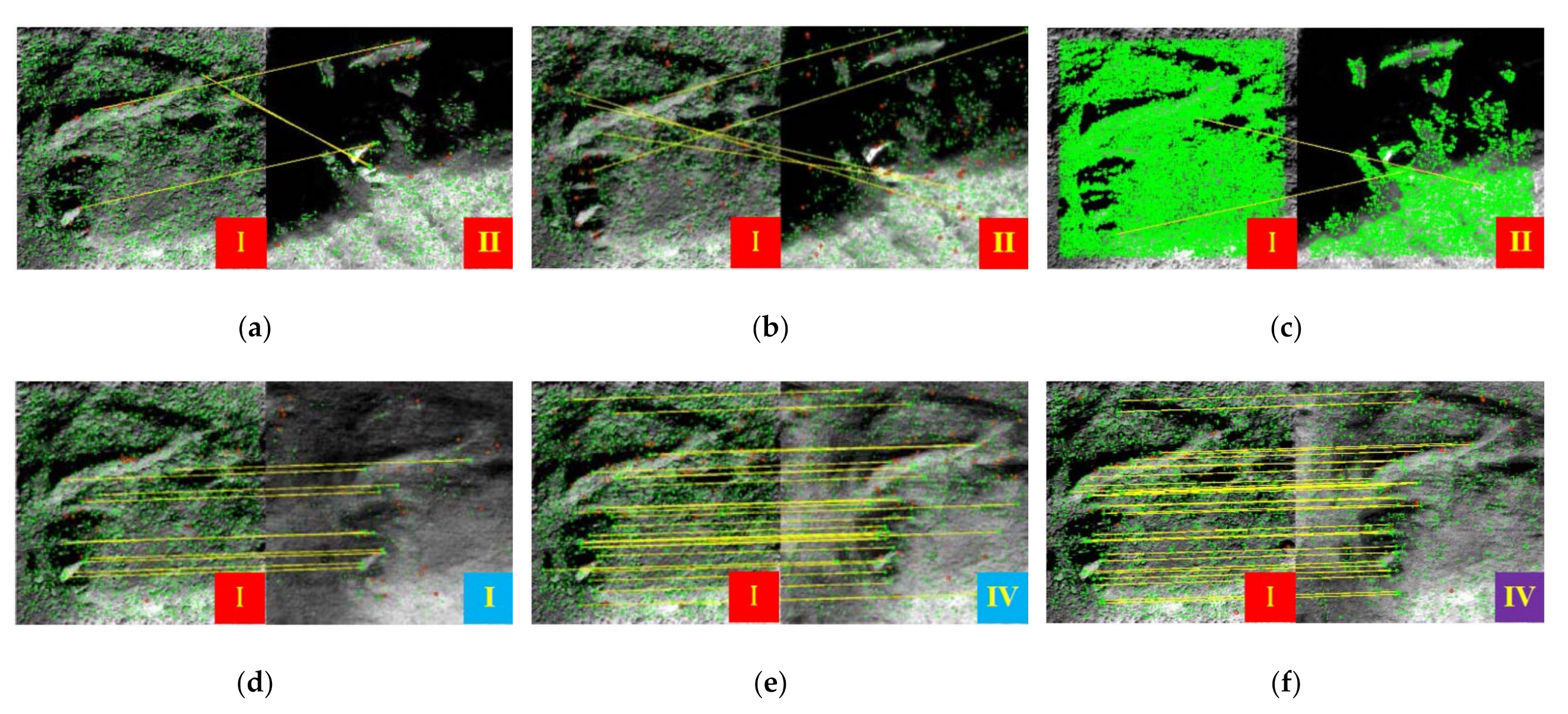
2.2.1. Match Outlier Filtering (MOF)

In the block feature matching phase, to deal with the high resolution, the sensed image and the reference image are divided into C1 × C2 blocks at equal intervals, respectively, and then the features are extracted and matched within the block. Block feature matching can improve the performance in two aspects: (1) through block feature matching, the feature area to be matched is reduced, so as to reduce the impact of low stable surface background noise and high self-similarity of vegetation texture, and improve the number and accuracy of feature-based matching. (2) In terms of computational performance, the block feature matching method reduces the overall computational complexity of the matching algorithm. In addition, the block feature matching method is also convenient for parallel calculation of each block and further improves the execution speed.

In order to improve the robustness of feature matching of complex texture background images, after consistency screening, we use MOF to filter and optimize the position of each inner point pair again, and record their RMI value of each group as the feature weight of the next local fitting. After feature distance matching (FDM) and random sample consensus screening (RANSAC) [46], the matching inner point pair is filtered by the intensity similarity threshold of the local area (taking the location of the feature point as the geometric center of local area). When the number of matching inner points is small, the template matching optimization of matching inner points is carried out based on the local area similarity index to further optimize the location of matching inner points. As shown in Figure 5, this method is suitable for the same resolution image registration with complex texture background.

Considering that regional mutual information (RMI) is an extension of mutual information [47], it combines spatial information in the form of energy function, and uses eight-neighbor information to calculate the joint probability distribution instead of the original gray information. Since RMI is robust to nonlinear intensity differences, and has been successfully applied to multispectral or multi-sensor image registration [23,24], we directly adopt it for the local area similarity measurement index:

$$P_0=P-\frac{1}{N}{{\displaystyle \sum }}_{i=1}^N{p}_i$$

(4)

$$C=\frac{1}{N}{P}_0{P}_0^T$$

(5)

$$RM\mathit{I}=H_g\left(C_A\right)+H_g\left(C_B\right)-H_g\left(C\right)$$

(6)

where $\mathit{P}=\left[{\mathit{p}}_1, {\mathit{p}}_2,\dots ,{\mathit{p}}_{\mathit{N}}\right]$,$N=\left(m-2r\right)\left(n-2r\right)$ is the number of pixels to be counted in a region, the size of the overlapping region is m × n, r is the radius of the local window, and ${\mathit{p}}_{\mathit{i}}$ is the pixel’s neighborhood vector for the i pixel. The size of P is d × N with d = 2 × r × r. $H_g\left(\mathit{C}\right)$ is the joint entropy. $H_g\left({\mathit{C}}_{\mathit{A}}\right)$ and $H_g\left({\mathit{C}}_{\mathit{B}}\right)$ are the marginal entropies, where ${\mathit{C}}_{\mathit{A}}$ is the (d/2) × (d/2) matrix in the upper left of C and ${\mathit{C}}_{\mathit{B}}$ is the (d/2) × (d/2) matrix in the lower left of C.

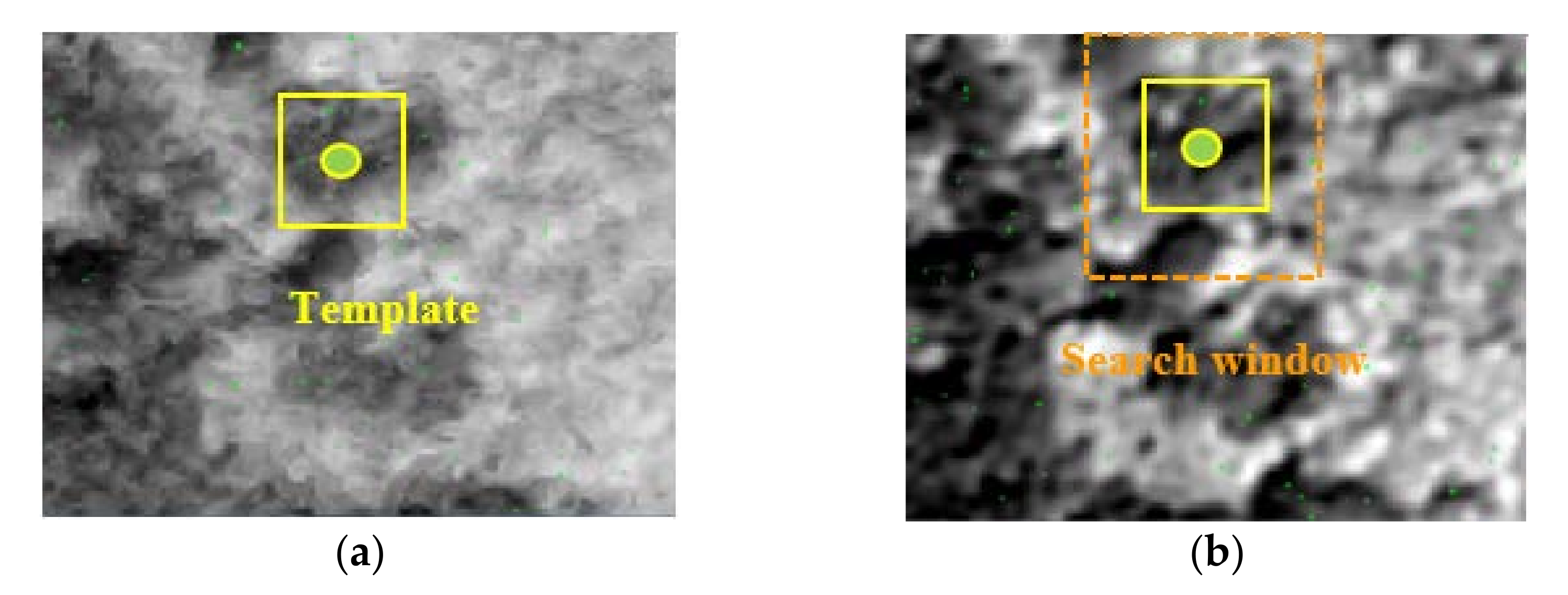
2.2.2. Dual-Weighted Block Fitting (DWBF)

Due to the low-stability and complex terrain, the accuracy of multi-temporal image feature matching is uncertain, and the uneven distribution of matching features is common. A block homography based on feature inverse distance weight (IDW) and feature region similarity weight (RSW) is proposed, which is called the dual-weighted block fitting (DWBF) method. First, the sensed image and the reference image are divided into C3 × C4 blocks at equal intervals, and each block corresponds to a separate homogeneous space homography transformation matrix $\mathit{H}\in {ℝ}^{3\times 3}$. Then, on the basis of a homography matrix estimation based on inner point pairs, the feature inverse distance weight [48] and feature similarity weight are added for each inner point pair. The feature inverse distance weight of each block is calculated based on the block center point ${\mathrm{x}}_{*}$. For any x of the matched inner point set, the farther the distance between ${\mathrm{x}}_{*}$ and x is, the lower the weight is when estimating the block homography matrix; the feature similarity weight is determined by the RMI of the region where the inner point is located, and the inner point with a high similarity has a higher influence weight.

Let $\mathrm{x}={\left(x,𝒴\right)}^{\mathrm{T}}$ and ${\mathrm{x}}^{\prime }={\left(x^{\prime },{𝒴}^{\prime }\right)}^{\mathrm{T}}$ be matching points across overlapping images I and I′. A basic method to estimate H from a set of point matches ${\left\{{\mathrm{x}}_i,{{\mathrm{x}}^{\prime }}_i\right\}}_{i=1}^{\mathrm{K}}$ across I and I′ can be expressed as:

$$\underset{ \mathrm{h}}{\widehat{\mathit{H}}=\arg \min }{{\displaystyle \sum }}_{i=1}^K||{\mathit{a}}_{\mathit{i}}{\mathit{H}}^2||\underset{ \mathrm{h}}{=\arg \min }||\mathit{A}{\mathit{H}}^2|| \mathrm{s}.\mathrm{t}||\mathit{H}||=1$$

(7)

where ${\mathit{a}}_{\mathit{i}}\in {ℝ}^{2\times 9}$ is computed for the i-th datum $\left\{{\mathrm{x}}_i,{{\mathrm{x}}^{\prime }}_i\right\}$, and the matrix A $\in {ℝ}^{2N\times 9}$ is obtained by stacking vertically ${\mathit{a}}_{\mathit{i}}$ for all i. After introducing the IDW and RSW, the block homography matrix ${\mathit{H}}_{*}$ is estimated from the problem:

$$\underset{h}{{\mathit{H}}_{*}=\arg \min }{{\displaystyle \sum }}_{i=1}^K||w_{*}^i{\mathit{a}}_{\mathit{i}}\mathit{H}||{}^2\underset{ \mathrm{h}}{=\arg \min }||{\mathit{W}}_{*}\mathit{A}\mathit{H}||{}^2$$

(8)

$$w_{*}^i=exp\left(-\frac{||{\mathrm{x}}_{*}-{\mathrm{x}}_i||{}^2}{{\eta }_i{\sigma }^2}\right)$$

(9)

$${\eta }_i=RM\mathit{I}\left(area\left({\mathrm{x}}_i\right),area\left({\mathrm{x}}^{\prime }i\right)\right)$$

(10)

where, ${\mathrm{x}}_{*}$ is the coordinate of the center point of the block, $\mathsf{\sigma }$ is a scale parameter and the weight matrix ${\mathit{W}}_{*}=\mathrm{diag}\left(\left[{\mathrm{w}}_{*}^1{\mathrm{w}}_{*}^1\cdots {\mathrm{w}}_{*}^N{\mathrm{w}}_{*}^N\right]\right)$. The problem in (8) is a weighted SVD problem, and the solution is simply the least significant right singular vector of ${\mathit{W}}_{*}$A.

2.3. Algorithm of CCFR

Based on the integration of LRC-BRE and BFM-LLT, CCFR can improve the overall restoration quality of a locally stable feature image sequence, and can select a more suitable local reference image for the local area of the sensing image rather than the global LRC-BRE application. The specific process of CCFR mainly includes three parts, as shown in Algorithm 1: (1) Batch coarse registration (steps 1–3). First, in order to reduce the complexity of feature matching and minimize the overall cost of spatial transformation of batch coarse registration, the image with the lowest outlier is selected as the common reference image of the whole image sequence G. Then, the BFM-LLT method is used to improve the alignment degree of coarse registration and realize the global alignment of most images. In the BFM step of rough registration, the matching results of each block are recorded as the guidance of whether the registered block participates in LRC-BRE. (2) Block-based LRC-BRE (steps 4 and 5). the LRC-BRE method is applied longitudinally to restore the block stable feature images for each block sequence after coarse alignment, and then they are synthesized into the global stable feature image horizontally. (3) Batch fine registration (step 6). With a globally stable feature image as a reference, the images are registered one by one using the BFM-LLT method.

Algorithm 1: CCFR

Input: images set${\left\{{\mathit{I}}_i^0\right\}}_{\mathrm{i}=1}^{\mathrm{N}}$

Step 1:${\left\{{\mathit{I}}_i^0\right\}}_{\mathrm{i}=1}^{\mathrm{N}}$ is aligned by geocoding, cropped and interpolated (optional) to obtain a group of image sequences G with the same size and the same resolution:

$\mathit{G}={\left\{{\mathit{I}}_{\mathit{i}}\right\}}_{i=1}^N\in {ℝ}^{\mathrm{w}\times \mathrm{h}}$

Step 2: The lowest outlier image ${\mathit{I}}_{\phi }$ from image sequence G is calculated by:

${\mathit{I}}_{\phi }=\underset{1\le i\le N}{ \arg \min }{{\displaystyle \sum }}_{j=1}^N\mathrm{diff}\left({\mathit{I}}_{\mathit{i}},{\mathit{I}}_{\mathit{m}\mathit{e}\mathit{a}\mathit{n}}\right)$

Step 3: With ${\mathit{I}}_{\phi }$ as the reference image, based on the BFM-LLT method, the image pairs $({\mathit{I}}_{\mathit{i}},{\mathit{I}}_{\phi }) i\in \left\{1,\dots ,N\right\} \mathrm{and} i\ne \phi$ are coarsely registered in turn to obtain a new image sequence ${\mathrm{G}}^{\prime }={\left\{{{\mathit{I}}^{\prime }}_{\mathit{i}}\right\}}_{i=1}^N$, and the matching results are recorded in the matrix set $\Lambda ={\left\{{\mathit{A}}_i\right\}}_{i=1}^N\in boo{l}^{C_1\times C_2}$:

$({{\mathit{I}}^{\prime }}_{\mathit{i}},{\mathit{A}}_{\mathit{i}})=$ BFM-LLT (${\mathit{I}}_{\mathit{i}},{\mathit{I}}_{\phi },C_1,C_2$)

where ${\mathit{I}}_{\mathit{i}}\in \mathit{G}$$, {{\mathit{I}}^{\prime }}_{\mathit{i}}$$=\left[\begin{array}{ccc}{\Omega }_i^{1,1}& \cdots & {\Omega }_i^{1,{\mathit{C}}_2}\\ ⋮& \ddots & ⋮\\ {\Omega }_i^{{\mathit{C}}_1,1}& \cdots & {\Omega }_i^{{\mathit{C}}_1,{\mathit{C}}_2}\end{array}\right]$$, {\mathit{A}}_{\mathit{i}}=\left[\begin{array}{ccc}{a}_i^{1,1}& \cdots & a_i^{1,C_2}\\ ⋮& \ddots & ⋮\\ a_i^{C_1,1}& \cdots & a_i^{C_1,C_2}\end{array}\right]$, ${\Omega }_{\mathit{i}}^{\mathit{j},\mathit{k}}\in {ℝ}^{w_{\mathsf{\Omega }}\times h_{\mathsf{\Omega }}}$ represents the block region in row j and column k of the image ${{\mathit{I}}^{\prime }}_{\mathit{i}}$, and $a_i^{j,k}$ represents the feature matching result of the block region in row j and column k of the image ${\mathit{I}}_{\mathit{i}}$. When the number of matching inner points in the region is insufficient, there is $a_i^{j,k}=$ true.

Step 4: Generate a stable feature image block sequence for each block sequence:${\left\{{\Omega }_{\mathit{i}}^{\mathit{j},\mathit{k}},{\Psi }_{\mathit{i}}^{\mathit{j},\mathit{k}},{\Gamma }_{\mathit{i}}^{\mathit{j}\mathit{,}\mathit{k}}\right\}}_{i=1}^N=\underset{{\mathit{L}}_{{\Omega }^{\mathit{j}}},{\mathit{S}}_{{\Omega }^{\mathit{j}}}}{\min } ||{\mathit{L}}_{{\Omega }^{\mathit{j},\mathit{k}}}||{}_{*}+\frac{1}{\sqrt{w_{\Omega }\times h_{\Omega }}}||{\mathit{S}}_{{\Omega }^{\mathit{j}},\mathit{k}}||{}_1 \mathrm{s}.\mathrm{t}. ||{\mathit{M}}_{{\Omega }^{\mathit{j},\mathit{k}}}-{\mathit{L}}_{{\Omega }^{\mathit{j},\mathit{k}}}-{\mathit{S}}_{{\Omega }^{\mathit{j},\mathit{k}}}||{}_{\mathrm{F}}\le ϵ$ where ${\mathit{M}}_{{\Omega }^{\mathit{j},\mathit{k}}}=\left[\mathrm{vec}\left({\Omega }_1^{\mathit{j},\mathit{k}}\right)\left|\cdots \right|\mathrm{vec}\left({\Omega }_{\mathit{q}}^{\mathit{j},\mathit{k}}\right)\right]\in {ℝ}^{m_{\Omega }\times q},m_{\Omega }=w_{\Omega }\times h_{\Omega },{\Omega }_{\mathit{i}}^{\mathit{j},\mathit{k}}\in {\mathit{G}}_{{\Omega }^{\mathit{j},\mathit{k}}}^{\mathit{q}},{\mathit{G}}_{{\Omega }^{\mathit{j},\mathit{k}}}^{\mathit{q}}={\left\{{\Omega }_{\mathit{i}}^{\mathit{j},\mathit{k}}\right\}}_{i=1}^q\left(q\le N\right)={\left\{{\Omega }_{\mathit{i}}^{\mathit{j},\mathit{k}}|a_i^{j,k}==true\right\}}_{i=1}^N,$${\Psi }_{\mathit{i}}^{\mathit{j},\mathit{k}}$ and ${\Gamma }_{\mathit{i}}^{\mathit{j},\mathit{k}}$ respectively represent the block stable feature image and block sparse matrix re-stored corresponding to ${\Omega }_{\mathit{i}}^{\mathit{j},\mathit{k}}$, and ϵ is a penalty factor.

Step 5: For each ${\mathit{I}}_{\mathit{i}}\in \mathit{G}$, its globally most suitable stable feature image ${\mathit{Z}}_{\mathit{i}}^{*}$ is synthesized by:

${\mathit{Z}}_{\mathit{i}}^{*}$$=\left[\begin{array}{ccc}{\Psi }^{*}{}_i^{1,1}& \cdots & {\Psi }^{*}{}_i^{1,{\mathit{C}}_2}\\ ⋮& \ddots & ⋮\\ {\Psi }^{*}{}_i^{{\mathit{C}}_1,1}& \cdots & {\Psi }^{*}{}_i^{{\mathit{C}}_1,{\mathit{C}}_2}\end{array}\right]$

where ${\Psi }_{\mathit{i}}^{*\mathit{j},\mathit{k}}=\mathrm{Best}\left({\Omega }_{\mathit{i}}^{\mathit{j},\mathit{k}},{\left\{{\Omega }_{\mathit{l}}^{\mathit{j},\mathit{k}},{\Psi }_{\mathit{l}}^{\mathit{j},\mathit{k}}\right\}}_{l=1}^q\right)$ is the most appropriate block stable feature image for ${\Omega }_i^{j,k}$. The Best () is given in Formula (1).

Step 6: Block feature matching and local linear transformation are carried out on the image pair $({{\mathit{I}}^{\prime }}_{\mathit{i}},{\mathit{Z}}_{\mathit{i}}^{*}) i\in \left\{1,\dots ,N\right\}$ in turn to obtain the accurately registered image sequence:

$({{\mathit{I}}^{″}}_{\mathit{i}},{{\mathit{A}}^{\prime }}_{\mathit{i}})=$ BFM-LLT (${{\mathit{I}}^{\prime }}_{\mathit{i}},{\mathit{Z}}_{\mathit{i}}^{*},{C^{\prime }}_1,{C^{\prime }}_2$)

output:${\left\{{{\mathit{I}}^{″}}_{\mathit{i}}\right\}}_{i=1}^N$

3. Results and Evaluations

In this section, three representative groups of HMR-LC images in

Table 1. Overview of the experimental data.

Type	Time	No.	Size	Res 1	Characteristics	Preprocessing	BFM Method
Ecological reserve	2015–2020	18	3600 × 3900 pixels	0.8 m	Mountainous areas with high vegetation coverage; deciduous vegetation is widely distributed.	Geocoding alignment + ortho-rectification (30 m precision DEM)	SURF 6 × 6 block
Mine production	2015–2021	18	2850 × 3300 pixels	0.8 m	Large-scale mining and waste discharge; evergreen vegetation and deciduous vegetation are staggered.	Geocoding alignment + ortho-rectification (30 m precision DEM)	SIFT 3 × 3 block
Mine environmental treatment	2014–2020	22	3900 × 4000 pixels	0.8 m	Small-scale mining activities, greening treatment, deciduous vegetation is widely distributed	Geocoding alignment	SIFT 5 × 5 block

¹ “Res” represents the spatial resolution.

were used to evaluate the proposed algorithm. By visual judgment and quantitative evaluation, the superior performance and the broad applicability of the proposed method in batch registration for HMR-LC images was verified.

3.1. Experimental Data and Related Algorithms

The high resolution satellite images used in the experiments are from the GF-2 satellite launched by China Aerospace Science and Technology Corporation (CASC). The satellite is a solar synchronous return orbit satellite with a short return cycle. It has been put into use in 2014. So far, it has accumulated a large number of multi-temporal high resolution images in the target area. We selected the panchromatic image of the satellite with high resolution (0.8 m) for correlation registration experiment. The three groups of images were aligned and cropped by using the geocoding information of the satellite images. Among them, the images of the ecological reserve and mine production area were ortho-rectified with 30 m precision DEM. Due to the limitation of positioning and model accuracy, there were still different degrees of alignment errors in the image sequence after course registration.

Three image sequence sets of complex terrain areas with different types of low-stability features were selected in the experiment. Among them, the ecological reserve is an ecological protection area dominated by natural landscape, and the unstable features are mainly the seasonal changes of vegetation such as deciduous trees and shrubs. The mine production area belongs to an iron mine area under production, and the unstable features are mainly concentrated in the mining area and waste discharge area. The mine environmental treatment area had experienced large-scale limestone surface mining before 2010. During the imaging period, there were only sporadic mining activities in this area, and greening treatment was started in some areas. Unstable features are mainly small-scale surface excavation, manual treatment, and seasonal changes of vegetation. The three experimental areas have the characteristics of complex terrain, large imaging time span, and large changes of land-cover in different time sequences.

In the visual evaluation part, we displayed and compared the results of stable feature image recovery, feature matching, and image alignment in three types of regions. In the quantitative evaluation part, the number of feature matching inner points of the global image sequence in each type of region is compared and analyzed. Through normalized correlation coefficient (NCC), mutual information (MI), and root mean square error (RMSE), the registration results of different types of low-stability remote sensing images are compared and analyzed.

The SIFT, SURF, and ORB algorithms are used in feature extraction and matching. After matching based on the sum of squared differences (SSD) of the feature, all three algorithms use consistency screening to purify matching points. For all the experiments, the RANSAC threshold was 0.1.

In the registration display, we compared the proposed method with the following four registration algorithms: The registration method by rank minimization (RRM) [49], piecewise linear mapping (PLM) [50], optical flow modification (OFM) [13], and as-projective-as-possible (APAP) [48]. RRM uses the low-rank structure as an effective constraint for registration tasks. In the experiment, the RRM patch size is set to the same size as the feature matching block. The PLM integrated into ENVI estimates the local affine transformation model for every triangle with three feature points. In PLM, the auto tie point generation matching method is cross-correlation. OFM uses optical flow field estimation and abnormal optical flow modification for remote sensing image registration for complex terrain areas. Due to the weak ability of the optical flow algorithm to deal with large displacement, we first used SIFT to obtain global parameters in the OFM experiment. The APAP algorithm uses the moving direct linear transformation (MDLT) method to estimate the local parameters, by providing higher weights to the closer feature points and lower weights to the farther ones. The SIFT algorithm was used in APAP. The feature method used by CCFR, as well as the parameters for generating block stable feature images, are shown in Table 1.

In order to verify the effectiveness of the LRC-BRE method, we designed ablation experiments in the registration experiments of the ecological reserve and mine production areas. We assume that the image after geocoding alignment and ortho-rectification by 30 m precision DEM can effectively reduce the local distortion of complex terrain and better realize the basic alignment requirements of Hypothesis 2. Based on the above, we directly carried out LRC-BRE and batch registration according to the process shown in Figure 3, which is represented by LRC-BRE-BR subsequently. The feature extraction and fitting method used by LRC-BRE-BR is same to CCFR. Because the initial alignment of the mine environmental treatment area images without ortho-rectification was low, the effect of the ablation experiment was poor.

3.2. Visual Quality

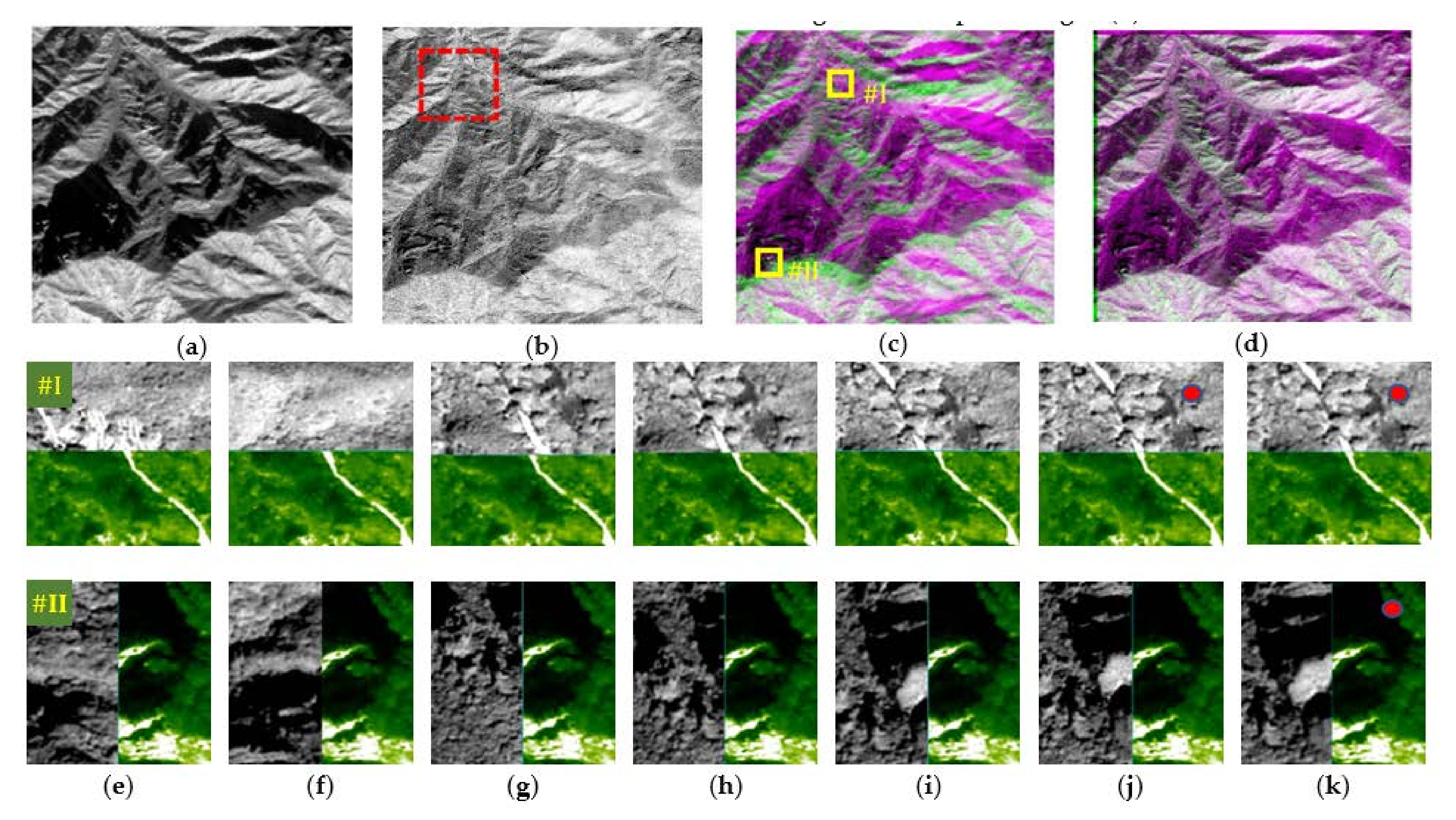
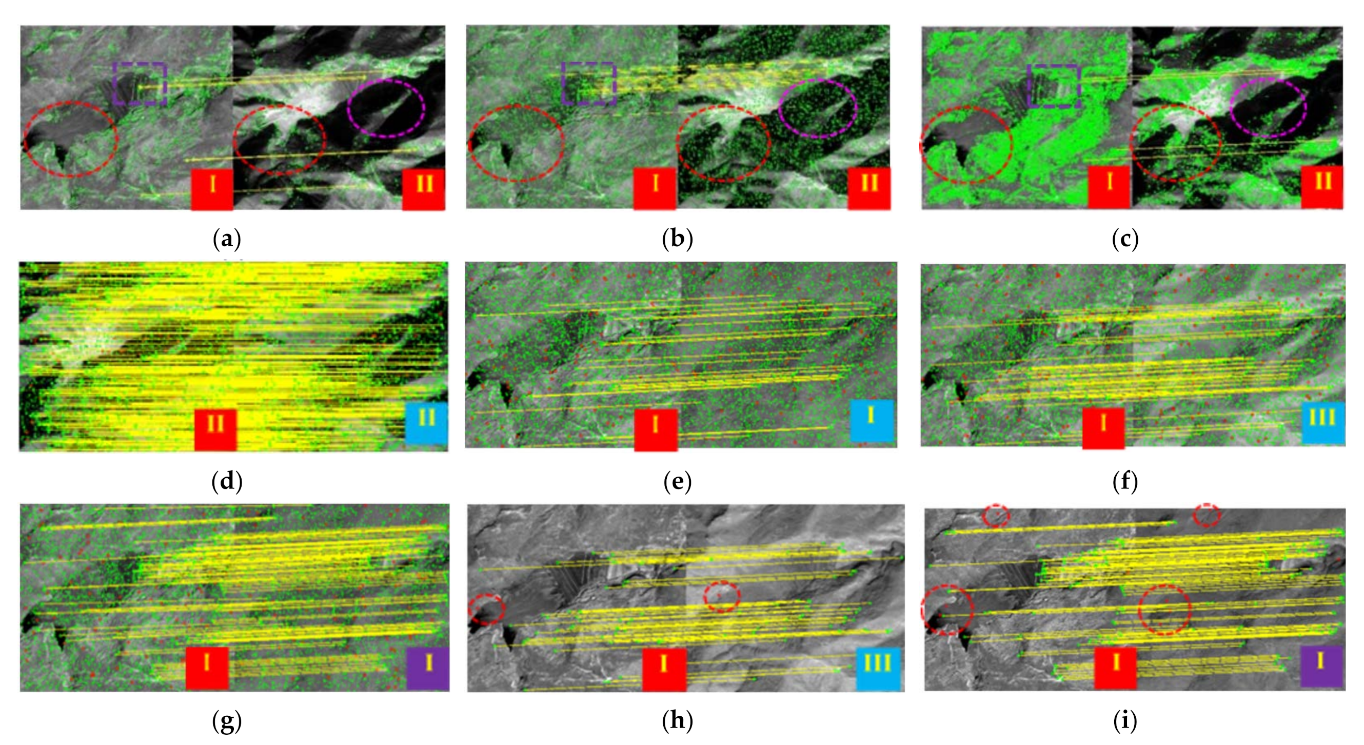
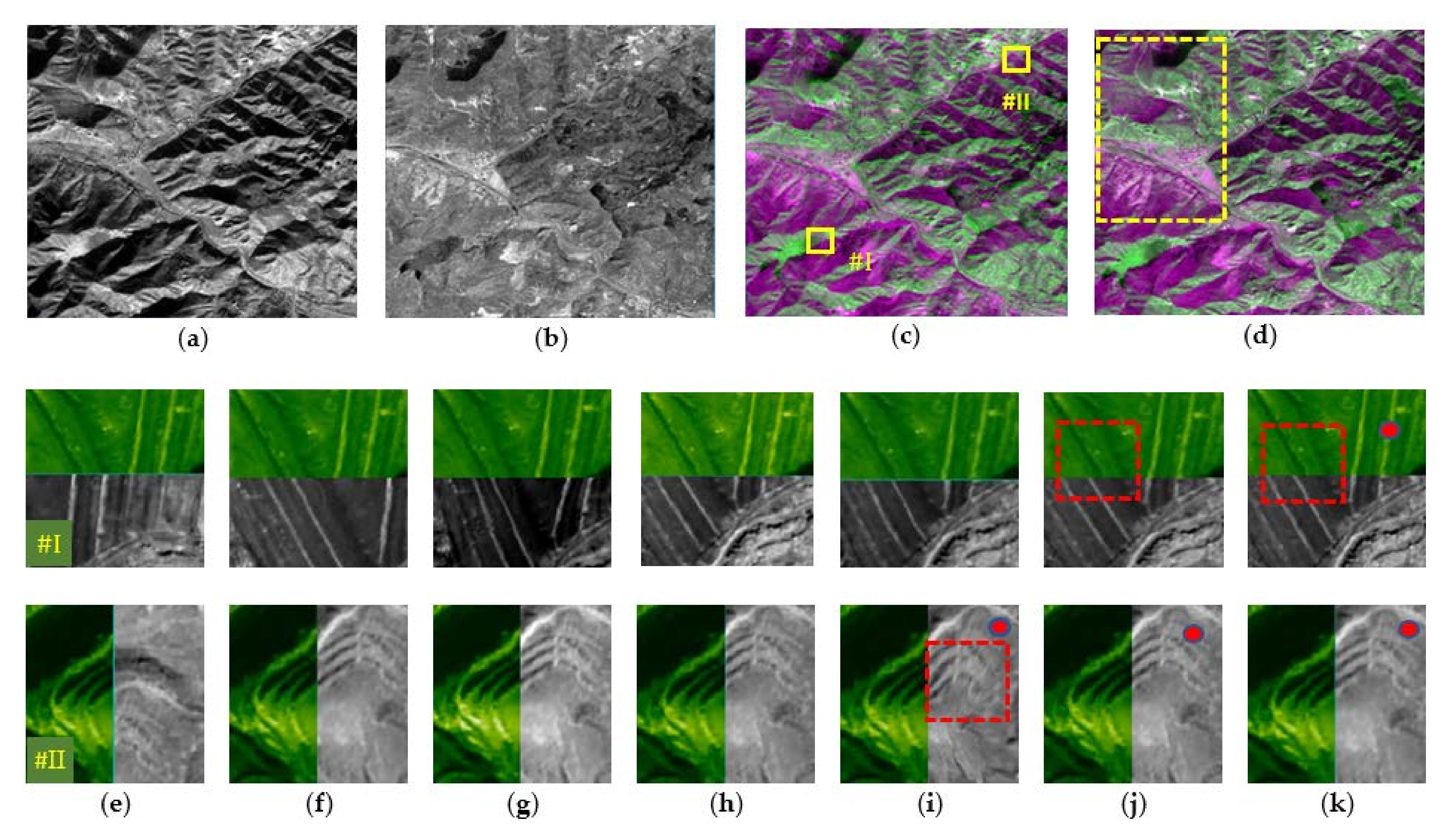
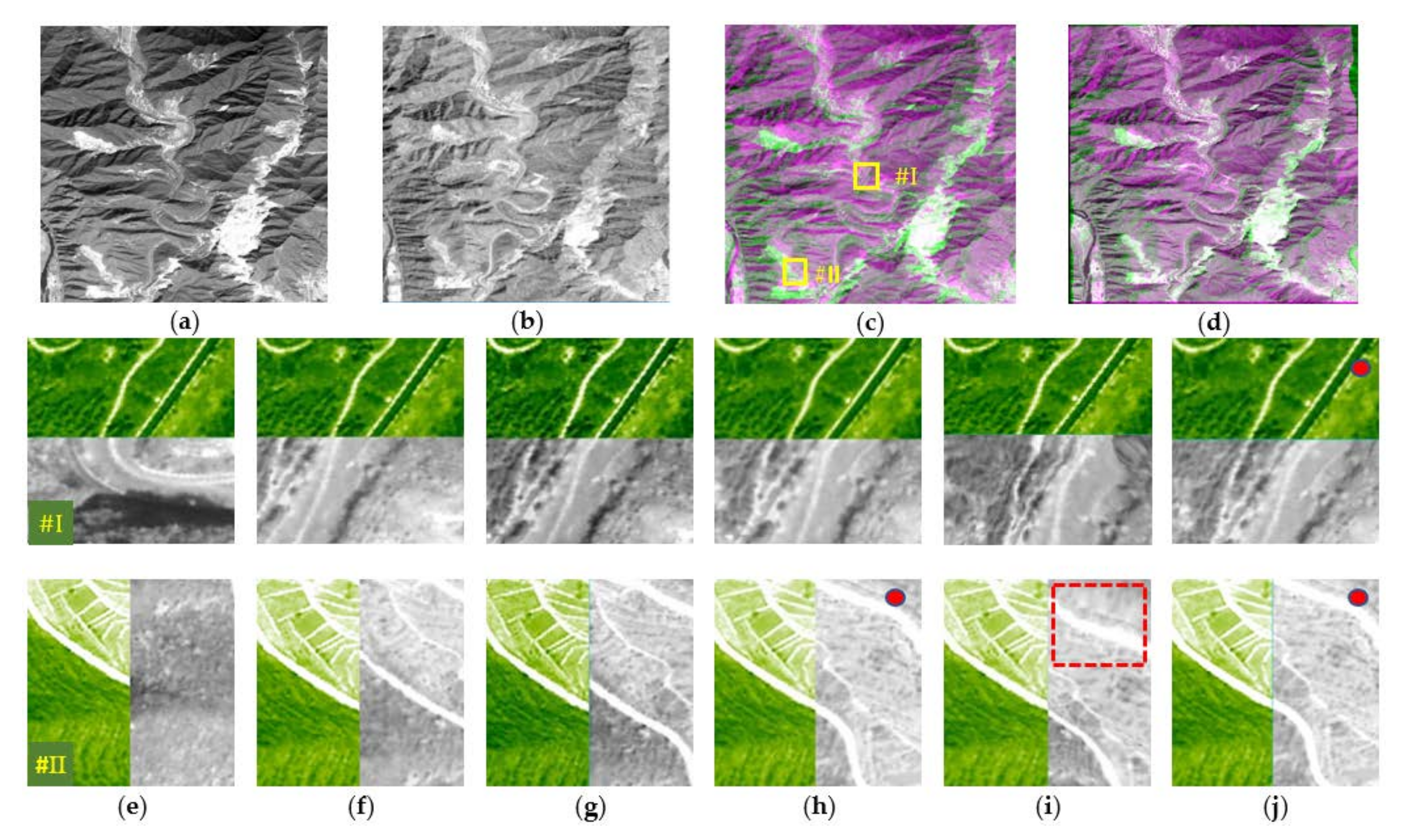
3.2.1. Ecological Reserve

Image restoration result: we used LRC-BRE and CCFR to restore stable feature images. Figure 6 shows the global mean image and local areas of the relevant results. The distortion of ground features in local areas is serious, and the mountains and rocks are raised. There are obvious differences in the contour, shadow and texture of ground features in different seasons. Figure 6a is the original image sequenced by ortho-rectification and geocoding alignment, which shows that there are a few large offset images (marked with a red box), and the offset direction is random. Figure 6b is the stable feature image sequence restored by the LRC-BRE. The results show that the stable feature image is clearly restored, and the unstable feature and temporary noise are removed. Including the image with large offsets in the initial alignment, all of the restored stable feature images are aligned in the spatial position. In addition, the comparison between the red boxes in Figure 6a,b shows that the texture difference between the original image with low alignment and the restored stable feature image is relatively large. Figure 6c is the stable feature image restored by CCFR, which is closer to the original image texture than Figure 6b; the difference is most significant in area V. Due to the failure of block feature matching in the coarse registration stage of CCFR, 6cI (marked with a blue box) did not generate the block stable feature image. Figure 6d is the final result of batch alignment using CCFR, showing that all local images have good spatial alignment.

Feature matching result: In the experiment, we selected two cross-seasonal local area images from the original image of the ecological reserve. Figure 7a–c are the results of features extracted and matching of image pairs (Figure 6aI imaged in August 2017 and Figure 6aII imaged in November 2019) through the SURF, SIFT, and ORB algorithms, respectively, showing that the number of matching inner points (yellow line segment connection points) obtained by the three feature matching algorithms was small and the error rate was high. Figure 7d–f are respectively the results of feature matching by the SURF algorithm between Figure 6aI with its corresponding stable feature image restored by LRC-BRE (Figure 6bI), the best alternative stable feature image extracted by LRC-BRE (Figure 6bIV), and the best alternative stable feature image extracted by CCFR (Figure 6cIV). The results show that the three groups of image pairs achieved correct feature matching, and the number of matching inner points increased in turn. Figure 7g–i respectively show the feature matching by SURF between Figure 6aII and the corresponding stable feature image restored by LRC-BRE (Figure 6bII), the best alternative stable feature image restored by LRC-BRE (Figure 6bIII), and the corresponding stable feature image restored by CCFR (Figure 6cII). The results show that the three groups of image pairs achieved correct feature matching, and the number of matching inner points increased in turn.

Image registration result: Taking the global image in Figure 8a of Figure 6aI as the reference image and the global image in Figure 8b of Figure 6aII as the sensed image, comparative experiments were carried out using different registration methods. Figure 8c is the overlay of Figure 8a,b, which is fuzzy and shows that there is still much ghosting caused by the offset after geocoding registration and ortho-rectification. Figure 8d is made up of the reference image and the aligned results by CCFR, in which the ghosting is basically eliminated. In order to further evaluate the registration results of different algorithms, the yellow rectangular region of the reference image and the results of the RRM, PLM, APAP, OFM, LRC-BRE-BR, and CCFR algorithms are enlarged, respectively. Figure 8e is an enlarged view of the yellow area of Figure 8c, with a large position offset in both vertical and horizontal directions. Figure 8f–i show that the results of the relevant registration algorithm have different degrees of offset in both the vertical and horizontal directions. Among them, the RRM method (Figure 8f) has the largest alignment error. Due to the obvious difference between images and textures, the tie point automatically generated by PLM using regional cross-correlation is not ideal, and the alignment result (Figure 8g) has a large offset. As the area is dominated by a natural landscape with few significant features, the correctly matched inner points obtained by SIFT are very few and unevenly distributed, and are mainly concentrated in the upper left area with roads (Figure 8b, red dotted line area). Therefore, the alignment offset of the APAP method (Figure 8h) in area #II is much larger than that in area #I. The OFM algorithm (Figure 8i) corrected and weakened the alignment error of area #II to some extent. After batch registration using the CCFR method (Figure 8k), the alignment of the target image pairs performed well. LRC-BRE-BR (Figure 8j) alignment results take the second place. For example, the stones in the central area (at the junction of gray and green) in Figure 8jII have a small lateral offset to the right with respect to Figure 8kII.

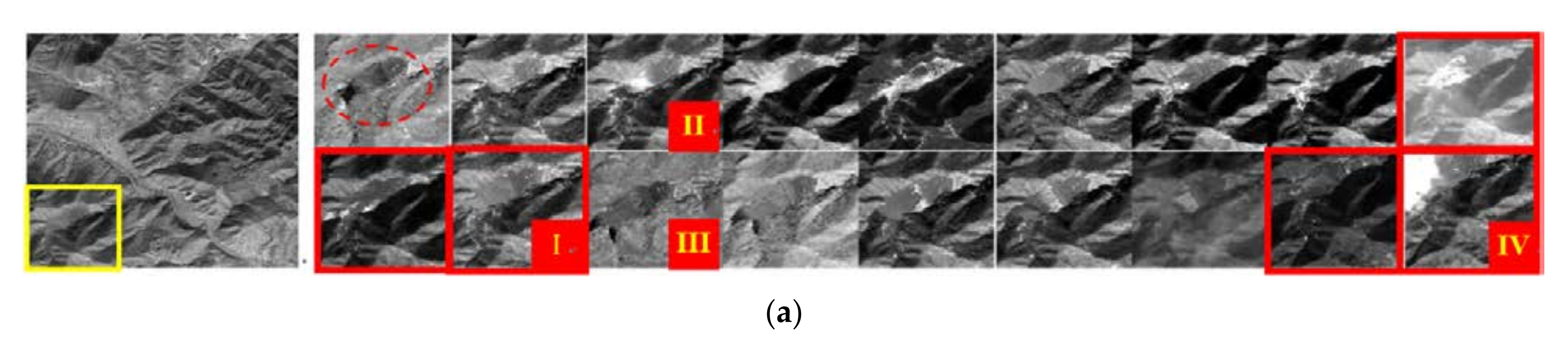
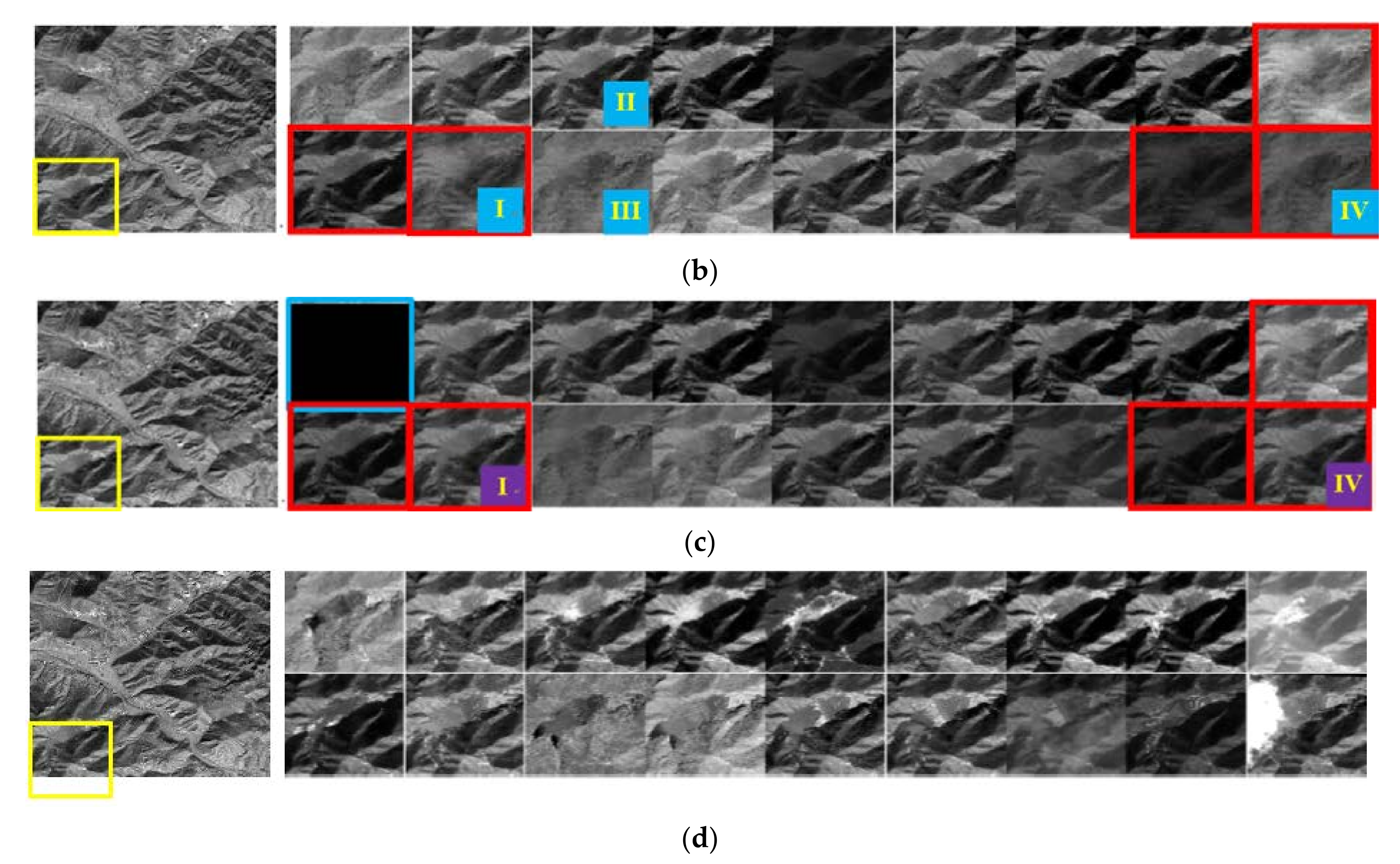
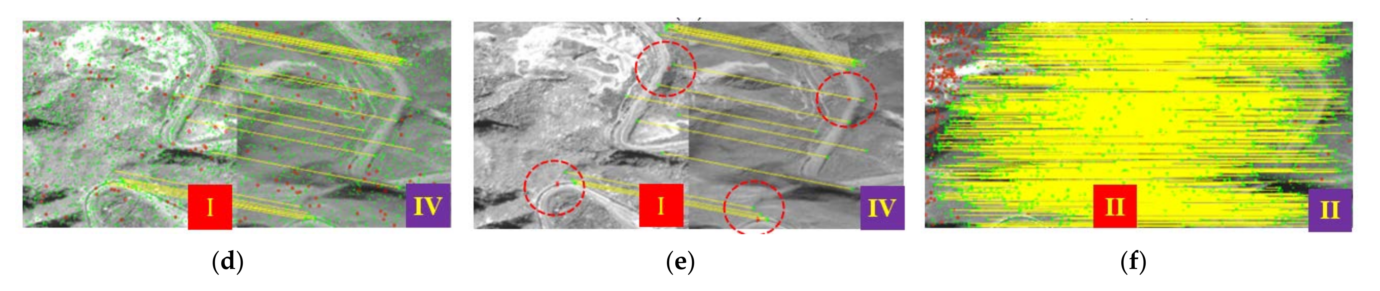
3.2.2. Mine Production Area

Image restoration result: In the right local areas of the original image sequence shown in Figure 9a, the ground features are mainly a tailings pond (marked by a red circle) with smelting waste. With the discharge of iron ore production waste, the edge area of the tailings pond is constantly changing, and the water content of deposits in tailings pond is also changing. Figure 9a shows that there are a few large offset images (marked with a red box), and the offset direction is random. Figure 9b is the stable feature image sequence restored by LRC-BRE, which shows that the topographic features of the overlapping area are recovered and the temporary interference noise (such as clouds and shadows in Figure 9bIV) is removed. The textures of some stable feature images in Figure 9b restored form the original large offset images (marked with a red box) are fuzzy. However, the textures of the stable feature images in Figure 9c restored by CCFR form the original large offset images (marked with a red box) are clear, and their spatial positions are aligned. Figure 9d shows that all images after batch registration by CCFR are spatially aligned well.

Feature matching result: In the experiment, we selected two local area images with a large time span from the original image sequence of mine production. Figure 10a–c are the results of features extracted and matching of the image pair (Figure 9aI imaged in June 2020 and Figure 9aII imaged in December 2016) through the SURF, SIFT, and ORB algorithms respectively, showing that the number of matching inner points is small and the distribution is very uneven, most of which are concentrated in the tailings dam area at the upper right (marked by a purple box). Due to the continuous discharge of semi fluid slag waste in the edge area of the tailings pond (marked by a red circle), where the image texture difference is obvious and the number of matching inner points is small. The shadow occlusion area on the right side of the image (marked by a magenta circle) also does not obtain the matching feature inner points. Figure 10d shows that due to the good initial alignment and lower vegetation noise interference in the winter image, the SIFT feature matching inner points of Figure 9aII and its corresponding stable feature image (Figure 9bII) restored by LRC-BRE are dense. Figure 10e–g are the SIFT feature matching of Figure 9aI with its corresponding stable feature image (Figure 9bI) restored by LRC-BRE, the best alternative stable feature image (Figure 9bIII) restored by LRC-BRE, and its corresponding stable feature image (Figure 9cI) restored by CCFR, respectively. The results show that the matching inner points obtained by the three groups of image pairs have a uniform distribution, the number of which increases in turn. Figure 10h,i shows the results of purifying the inner points in Figure 10f,g respectively, by MOF, and the inner points with a large offset in the red circle area are eliminated.

Image registration result: Different registration methods were carried out with the global image in Figure 11a of Figure 9aI as the reference image and the global image in Figure 11b of Figure 9aII as the sensed image. Figure 11c is the overlay of Figure 11a,b, which shows that there is still much ghosting caused by certain offsets after geocoding registration and ortho-rectification. Figure 11d shows that the ghosting of the global image pair after registration using the CCFR algorithm is weakened and the texture of the yellow dotted line area is clearer, but the ground surface in the lower left area changes significantly due to surface mining, tailings discharge, land cultivation, and other reasons. Figure 11e is an enlarged view of the yellow area of Figure 11c, with a large position offset in both vertical and horizontal directions. Figure 11f–i show that the registration results of the RRM, PLM, APAP, and OFM algorithms have different degrees of offset, and the offset degree of region #I is generally larger than that of region #II. Figure 11f shows that the registration result of the RRM method has a large alignment error. Because some artificial features with high feature significance are distributed in the overlapping area, the alignment result of the APAP algorithm (Figure 11h) is relatively good. The alignment effect of the OFM algorithm (Figure 11i) is relatively good, but the registered image on the right side (marked by a red box) of region #II is over-stretched. After batch registration by LRC-BRE-BR (Figure 11j) and the CCFR method (Figure 11k), the alignment of the target image pair is good, and the image texture is not excessively stretched. The offset of the tailings dam section in the red box in area #I of Figure 11j,k belongs to the actual displacement of ground objects, which is related to the continuous heightening of the dam body to the left with the increase of tailings excreta.

3.2.3. Mine Environmental Treatment Area

Image restoration result: The image of the mine environmental treatment area is not ortho-rectified, and the initial alignment degree is low. CCFR was used for stable feature image restoration and batch registration in this area. LRC-BRE was only used to restore the stable feature image. The right side of Figure 12 is the local areas of the original image sequence and the stable feature image sequence recovered by different methods. The upper left corner of this local areas (for example, the red box in Figure 12a) is the quarry still being excavated during the imaging period, and the surface changed significantly over different periods. The right side of Figure 12a is the local areas of the original image sequence aligned by geocoding, showing that the initial alignment degree is low, and there are generally large offsets in the location of roads and quarries in the area. Its left global mean image texture is fuzzy and contains heavy ghosting. The right side of Figure 12b shows the local areas of the stable feature image recovered by the LRC-BRE method. The result shows that the image texture is blurred and the distortion is high. The right side of Figure 12c shows the local areas of the stable feature image recovered by the CCFR method. The results show that most areas recover the stable feature image, with clear ground objects and consistent spatial position. Only a few regions do not generate stable feature images. Figure 12d shows that all images after batch alignment using CCFR have been spatially aligned well, and the left global mean image texture is clear.

Feature matching result: In the experiment, we selected two local area images with a large time span but similar seasons from the original image sequence of the mine environmental treatment area. Figure 13a–c are the results of features extracted and the matching of image pairs (Figure 12aI imaged in late April 2020 and Figure 12aII imaged in early April 2016) through the SURF, SIFT, and ORB algorithms, respectively, showing that the number of matching inner points is small and the error rate is high. This is the main reason that the quarry area (marked by a red circle) in the image pair has changed significantly, although the seasonal change of vegetation and the change of solar altitude angle are small. Figure 13d shows that the number of SIFT feature matching inner points of Figure 12aI and the best alternative stable feature image (Figure 12aIV) recovered by CCFR is large and evenly distributed. In Figure 13d, there are still a few internal points with a position offset, which is effectively filtered by MOF in Figure 13e (marked by a red circle). Figure 13f shows that the SIFT feature matching inner points of Figure 12aII and its corresponding stable feature images recovered by CCFR are densely distributed.

Image registration result: Taking the global image in Figure 14a of Figure 12aI as the reference image and the global image in Figure 14b of Figure 12aII as the sensed image, comparative experiments were carried out using different registration methods. Figure 14c is the overlay of Figure 8a,b, which shows that there is much ghosting caused by the offset after geocoding registration. Figure 14d shows that the ghosting of the global image pair registered by the CCFR algorithm is significantly weakened, except that the image edge and some mining areas still have color superposition. Figure 14f–i shows respectively that the registration results of RRM, PLM, APAP, and OFM have different degrees of offset in area #I, which is related to the proximity of the mining area with obvious changes. The registration results of RRM (Figure 14f) and PLM (Figure 14g) also have obvious offsets in area #II. Since a small number of artificial objects with high feature significance are distributed near area #II, APAP (Figure 14h) and OFM (Figure 14i) achieve good alignment of trunk roads in area #II. However, the right resampled image (marked by a red box) of OFM (Figure 14i) in area #II has obvious tensile deformation. After batch registration by CCFR, the alignment of the target image pair (Figure 14j) is good, and the image is not excessively stretched.

From the visualization results of the above three groups of experiments, it can be seen that LRC-BRE and the block-based LRC-BRE (CCFR) are effective for extracting stable feature images as reference images. For the registration between original images and stable feature images extracted, the BFM-LLT method has good results in feature matching and local alignment. The CCFR method can realize the batch alignment of three different types of HMR-LC, and achieve better performance.

3.3. Evaluation of Registration Results

In order to evaluate the accuracy of the image registration, we used the normalized correlation coefficient (NCC), mutual information (MI), and root-mean-square error (RMSE) metrics to conduct the quantitative assessment. Both NCC and MI can reflect the degree of similarity between two images, and are popular evaluation indexes used in the quality assessment of image registration.

The NCC metric is used to provide an overall judgement as to whether the sensed image is well-aligned with the reference image [22,51]:

$$NCC\left({\mathit{I}}_1,{\mathit{I}}_2\right)=\frac{{{\displaystyle \sum }}_{i=1}^N[{\mathit{I}}_1\left(i\right)-\overline{{\mathit{I}}_1}]\left[{\mathit{I}}_2\left(i\right)-\overline{{\mathit{I}}_2}\right]}{\sqrt{{{\displaystyle \sum }}_{i=1}^N{[{\mathit{I}}_1\left(i\right)-\overline{{\mathit{I}}_1}]}^2}\sqrt{{{\displaystyle \sum }}_{i=1}^N{\left[{\mathit{I}}_2\left(i\right)-\overline{{\mathit{I}}_2}\right]}^2}}$$

(11)

where ${\mathit{I}}_1\left(i\right)$ and ${\mathit{I}}_2\left(i\right)$ are the intensity values of the i-th pixel in image ${\mathit{I}}_1$ and image ${\mathit{I}}_2$, respectively; and $\overline{{\mathit{I}}_1}$ and $\overline{{\mathit{I}}_2}$ are the corresponding average intensity values. N is the pixel number. The available range of NCC is [−1, 1], and NCC generally belongs to (0,1). A larger value of NCC indicates a more accurate registration result.

The MI metric is used as a cost function in similarity measure-based approaches to registration [52]:

$$M\mathit{I}\left({\mathit{I}}_1,{\mathit{I}}_2\right)={\displaystyle \sum }_{g_1\subset {\mathit{I}}_1}{\displaystyle \sum }_{g_2\subset {\mathit{I}}_2}{p}_{{\mathit{I}}_1,{\mathit{I}}_2}\left(g_1,g_2\right)log\left[\frac{p_{{\mathit{I}}_1,{\mathit{I}}_2}\left(g_1,g_2\right)}{p_{{\mathit{I}}_1}\left(g_1\right)p_{{\mathit{I}}_2}\left(g_2\right)}\right]$$

(12)

The available range of MI is (0, 2). A larger value of MI represents a more precise registration result.

The RMSE metric focuses on evaluating the registration result by calculating the average distance of the corresponding points in the reference and aligned image:

$$RMSE=\sqrt{\frac{1}{N}{\displaystyle \sum }_{i=1}^N{\left(\Delta x_i\right)}^2+{\left(\Delta y_i\right)}^2}$$

(13)

where N is the number of evaluated points, and $x_i$ and $y_i$ are the residual differences of the i-th checkpoint pair in the x and y directions. A smaller RMSE indicates a better result.

The three groups of experiments correspond to Figure 8, Figure 11 and Figure 14 of the visual evaluation experiment, respectively. The quantitative evaluation results are shown in

Table 2. Quantitative evaluation of the registration results in the three experiments.

	Ecological Reserve			Mine Production			Mine Environmental Treatment
	NCC	MI	RMSE/pixels	NCC	MI	RMSE/pixels	NCC	MI	RMSE/pixels
Original	0.28136	0.059138	0.37336	0.14756	0.026849	0.28831	0.28807	0.058247	0.27997
RRM	0.40549	0.10822	0.3533	0.27153	0.054601	0.26371	0.45068	0.13519	0.25229
PLM	0.50274	0.2535	0.31822	0.29541	0.093957	0.27233	0.49631	0.16344	0.24489
APAP	0.63317	0.32688	0.3533	0.34195	0.097451	0.25461	0.53916	0.19488	0.23318
OFM	0.6786	0.34853	0.30167	0.33511	0.09357	0.2557	0.50141	0.17111	0.24879
LRC-BRE-BR	0.68687	0.35448	0.31131	0.36022	0.10722	0.25249	null	null	null
CCFR	0.70928	0.39685	0.28171	0.38415	0.11548	0.24826	0.6413	0.30463	0.22609

.

According to Table 2, we can draw the following conclusions: (1) Quantitative evaluation of the same type of areas and different registration methods: Due to the global offset in the original image alignment of the three areas, the NCC and MI indicators are low, and the RMSE/pixels indicators are high. The registration result of the RRM algorithm is the worst, and there are generally large offsets. Only in the local area with significant features such as artificial objects, the feature-based APAP method achieves a relatively good alignment result. The registration indicators of the OFM algorithm are better than RRA and APAP. The proposed CCFR methods achieved the best quantitative evaluation. In the ecological reserve and mine production area by geocoding registration and ortho-rectification, the quantitative evaluation of LRC-BRE-BR is second only to CCFR. (2) Quantitative evaluation of the same registration method and different type areas: Since there are only seasonal vegetation changes in land-cover, the NCC and MI indicators of multiple registration methods in the ecological reserve are overall higher than those in the other two areas. Due to the large surface changes caused by mining and waste discharge, the NCC and MI indicators of multiple registration methods in the mine production area are lower than in the other two areas. The overall similarity of RMSE/pixels indicators to different regions is slightly inconsistent with NCC and MI. For example, the RMSE/pixels indicators of ecological reserves are the highest. However, the change trend of RMSE/pixels in the same area and the same registration method is consistent with NCC and MI. That is, the larger the NCC, the larger the MI and the smaller the RMSE/pixels.

In general, the CCFR method is effective for HMR-LC images’ registration. Especially when the land-cover changes and influence of radiation differences are significant, the robustness of CCFR is superior to other registration methods of comparison.

4. Discussion

The previous section validates the effect of the proposed method in image registration. This section discusses the advantages and influencing factors of indirect registration with stable feature images restored by LRC-BRE as the reference, and introduces the work of CCFR in different satellite images.

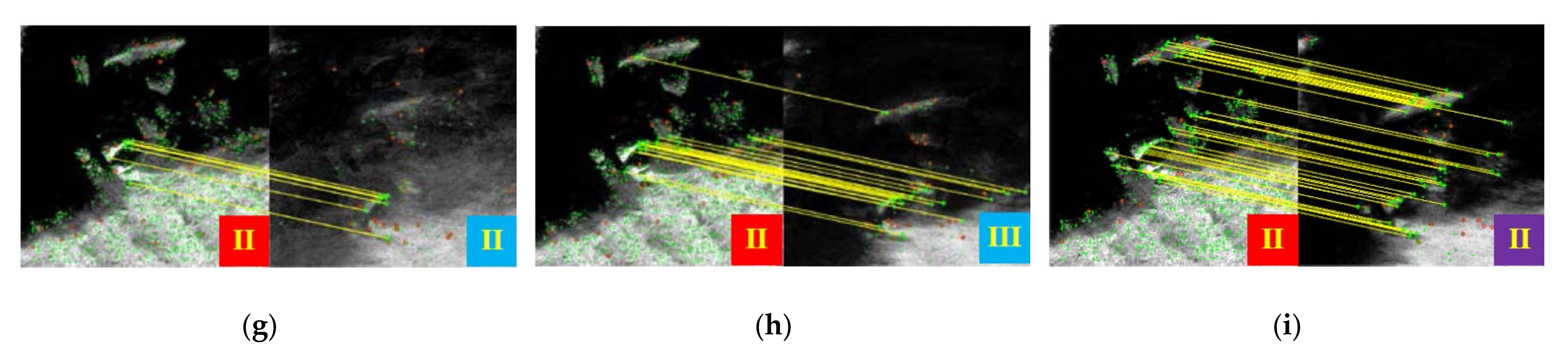
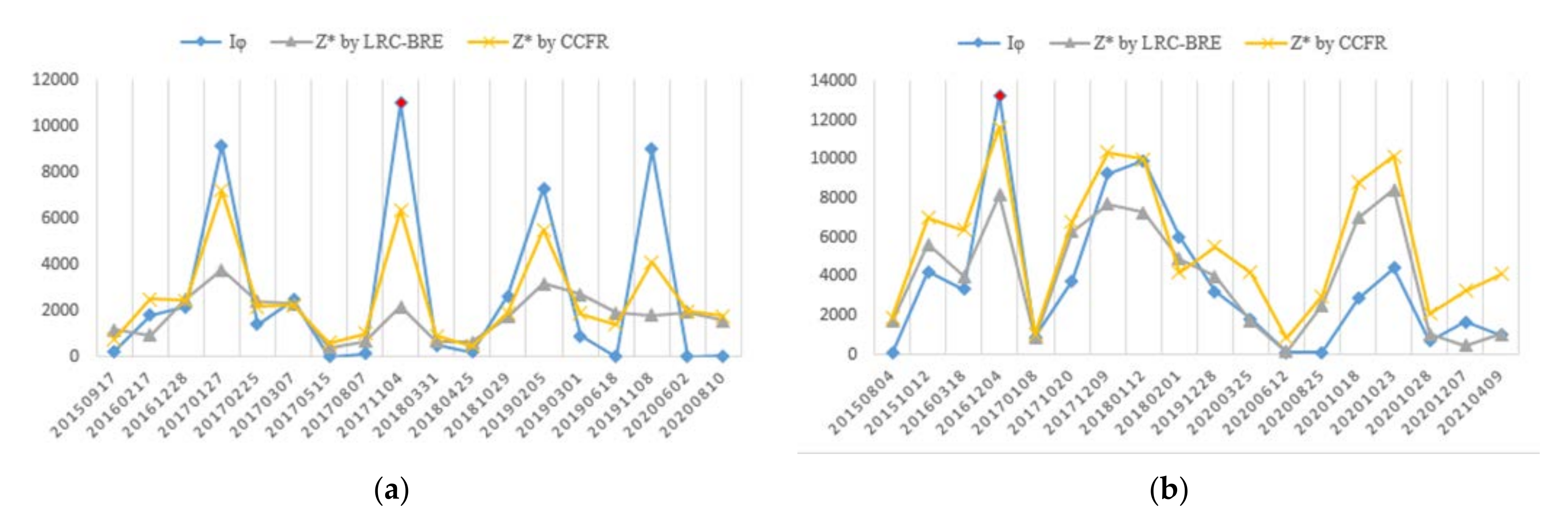
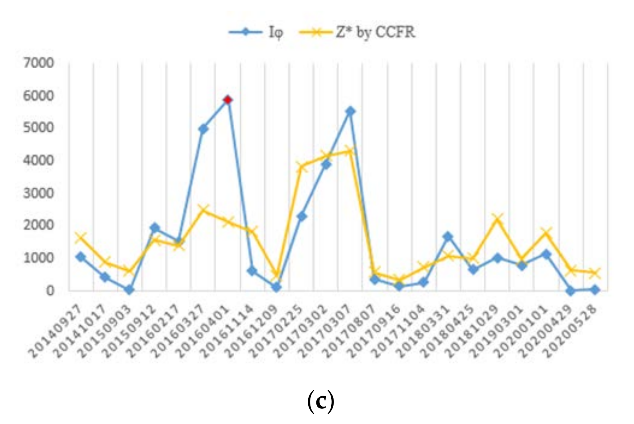
4.1. Quantitative Comparison of Feature Matching Results

In order to objectively verify the influence of the stable feature image as a reference image on feature matching, Figure 15 shows the results of direct feature matching and indirect feature matching with the reference of a stable feature image as the reference for the multi-temporal global image sequence in the three experimental areas in Section 3.2. For the image pairs with a small texture difference from the specified image ${\mathit{I}}_{\phi }$ in the sequence, the effect of direct feature matching is better; however, for the HMR-LC images sequence, the image pairs with small texture differences are relatively rare. Details are as follows:

For the ecological reserve image sequence, the statistics of matched inner points with BFM(SURF) are shown in Figure 15a. The results show that the number of inner points obtained by image pair (${\mathit{I}}_{\mathit{i}},{\mathit{I}}_{\phi }$) direct feature matching fluctuates greatly. The number of inner points between image pairs (${\mathit{I}}_{\mathit{i}},{\mathit{I}}_{\phi }$) imaged in the same or similar seasons is the largest among the three types of broken lines, but that between image pairs (${\mathit{I}}_{\mathit{i}},{\mathit{I}}_{\phi }$) imaged across seasons is lower than those of (${\mathit{I}}_{\mathit{i}},{\mathit{Z}}_{\mathit{i}}^{*\mathit{L}}$) and (${\mathit{I}}_{\mathit{i}},{\mathit{Z}}_{\mathit{i}}^{*\mathit{C}}$), or even close to 0. This is related to the large seasonal variation of deciduous woody vegetation in the area. The fluctuation of the number of inner points of the image pair (${\mathit{I}}_{\mathit{i}},{\mathit{Z}}_{\mathit{i}}^{*\mathit{L}}$) and (${\mathit{I}}_{\mathit{i}},{\mathit{Z}}_{\mathit{i}}^{*\mathit{C}}$) sequence is small, and the situations of broken line valleys is better than (${\mathit{I}}_{\mathit{i}},{\mathit{I}}_{\phi }$).

For of mine production area image sequence, the statistics of feature matching of inner points with BFM(SIFT) are shown in Figure 15b. The results show that only a few (${\mathit{I}}_{\mathit{i}},{\mathit{I}}_{\phi }$) with similar seasons have more inner points than those of (${\mathit{I}}_{\mathit{i}},{\mathit{Z}}_{\mathit{i}}^{*\mathit{L}}$) and (${\mathit{I}}_{\mathit{i}},{\mathit{Z}}_{\mathit{i}}^{*\mathit{C}}$) in the same period. In most cases, the number of inner points between (${\mathit{I}}_{\mathit{i}},{\mathit{Z}}_{\mathit{i}}^{*\mathit{C}}$) is the largest, and the number of inner points between (${\mathit{I}}_{\mathit{i}},{\mathit{Z}}_{\mathit{i}}^{*\mathit{L}}$) is the second. In addition to seasonal fluctuation of the number of inner points, due to the surface changes caused by the continuous large-scale mine production in the area during the imaging period, with increasing of the time interval from ${\mathit{I}}_{\phi }$ (red dot), the number of inner points of (${\mathit{I}}_{\mathit{i}},{\mathit{I}}_{\phi }$) shows an overall downward trend. However, the number of inner points in (${\mathit{I}}_{\mathit{i}},{\mathit{Z}}_{\mathit{i}}^{*\mathit{L}}$) and (${\mathit{I}}_{\mathit{i}},{\mathit{Z}}_{\mathit{i}}^{*\mathit{C}}$) is relatively stable.

For the mine environmental treatment area image sequence, the statistics of feature matching of inner points with BFM(SIFT) is shown in Figure 15c. The results show that the number of inner points between (${\mathit{I}}_{\mathit{i}},{\mathit{I}}_{\phi }$) with a large seasonal span is smaller than that between (${\mathit{I}}_{\mathit{i}},{\mathit{Z}}_{\mathit{i}}^{*\mathit{C}}$). In addition, the number of inner points of (${\mathit{I}}_{\mathit{i}},{\mathit{I}}_{\phi }$) and (${\mathit{I}}_{\mathit{i}},{\mathit{Z}}_{\mathit{i}}^{*\mathit{C}}$) decreases as the time interval from I (red dot) increases. This is related to the land-cover changes caused by the strengthening of mine ecological restoration in the region since 2018.

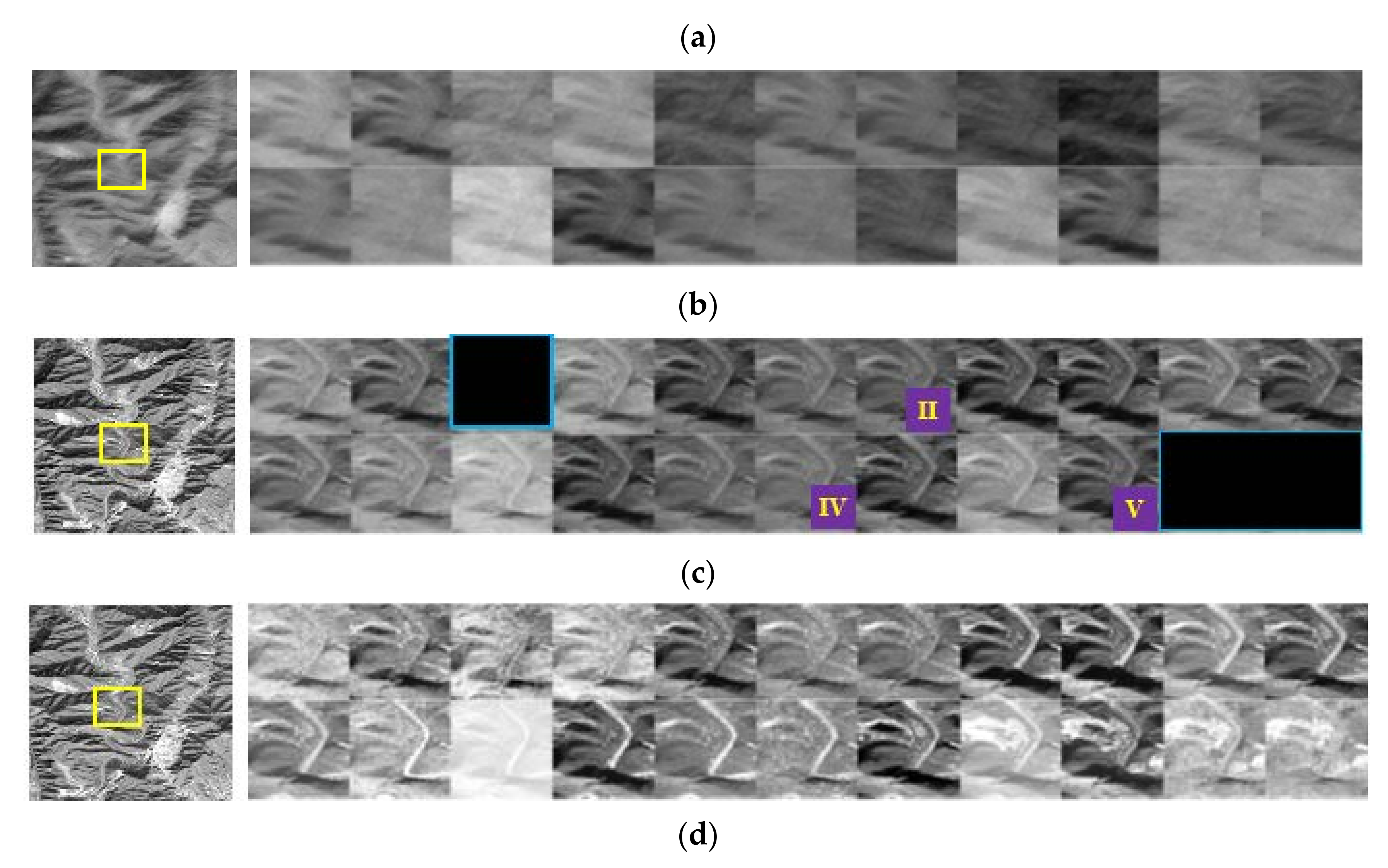
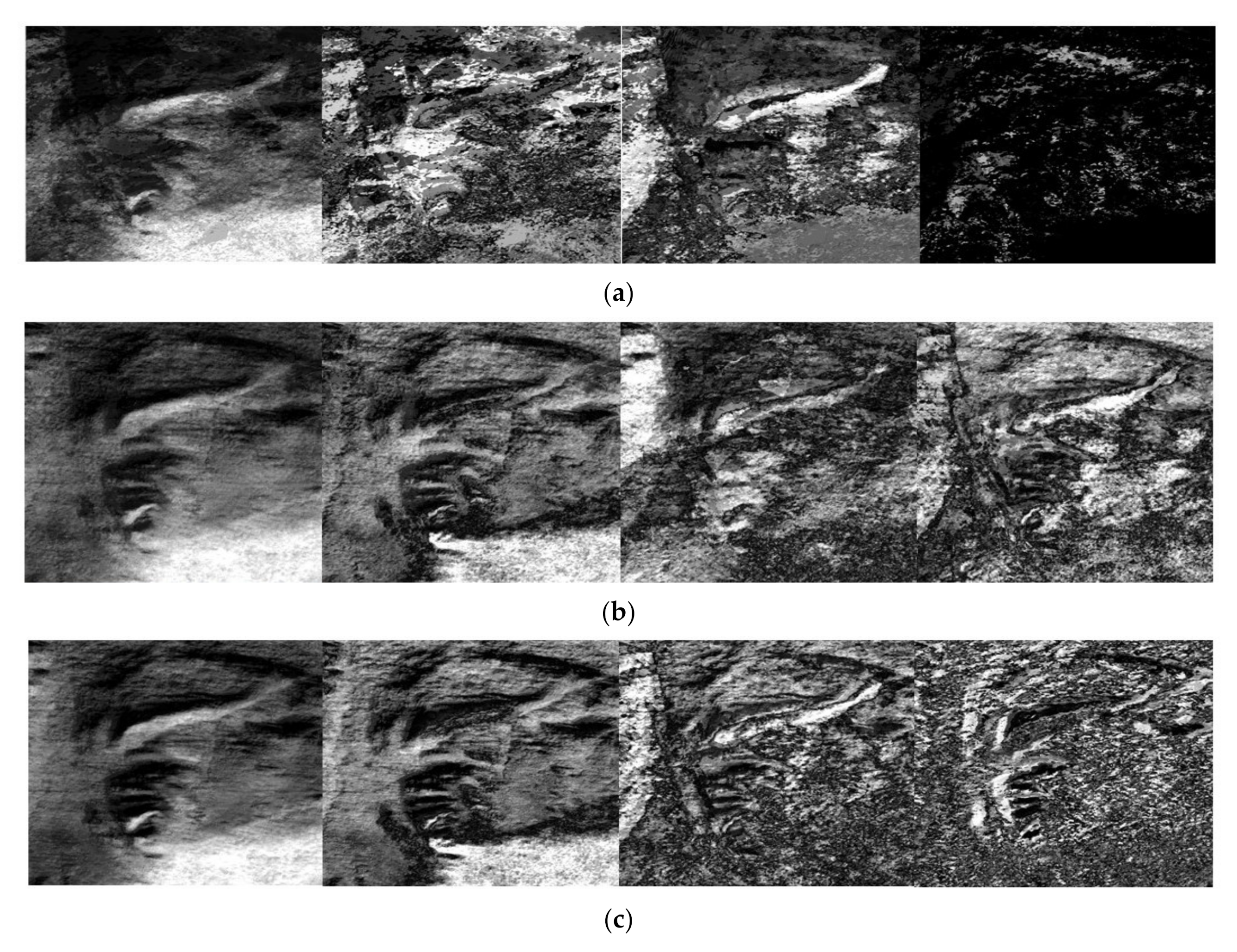
4.2. Correlation Factors of Restored Stable Feature Image Quality

According to Theorem A1 in the Appendix A, the restored stable feature image is composed of the first R principal component vectors ${\left\{{\mathit{u}}_{\mathit{i}}\right\}}_{i=1}^R$ generated by the low-rank decomposition from the initial image sequence. Moreover, the difference of the coefficient ${\left\{{\sigma }_i\right\}}_{i=1}^R$ corresponding to the principal component vector sequence is exponential. Therefore, the restored quality of the stable feature image sequence is closely related to the principal component vectors sorted in the front. In addition, according to the Inference A2 in the Appendix A, when the texture difference noise remains unchanged, the restoration quality of the stable feature image sequence is positively correlated with the spatial consistency of the initial image sequence.

To facilitate the discussion on the correlation factors of the restored stable feature image quality, taking the local image sequences of ecological reserves in Section 3.2.1 as an example, the texture states of images ${\mathit{D}}_{\mathit{i}}$ corresponding to the principal component vector ${\mathit{u}}_{\mathit{i}}$ extracted by low-rank decomposition from different initial image sequences are compared. The image ${\mathit{D}}_{\mathit{i}}$ is generated by the following:

$${\mathit{D}}_{\mathit{i}}=ve{c}^{-1}\left(abs({\mathit{u}}_{\mathit{i}})\right)$$

(14)

where abs(.) means taking an absolute value for each element of the vector, and ${\mathrm{vec}}^{-1}$ indicates the reverse operation of stacking. Figure 16a is the first four principal component images generated by low-rank decomposition from nine local images of the first row in Figure 6a, in which the proportion of large offset images (marked by a red box) is 2/9. Figure 16b was generated by low-rank decomposition from all 18 local images in Figure 6a, in which the proportion of large offset images (marked by a red box) is also 2/9. Figure 16c was generated from 16 local images (excluding severely outlying block images after coarse registration by CCFR) in Figure 6a.

Among the three groups of results in Figure 16, the texture features of principal component images (especially the first two) (Figure 16c) generated by the CCFR method are the clearest through rough registration based on blocks and eliminating the severely outlying block images used by low-rank decomposition. When the proportion of large offset images in the initial image set is the same, the principal component images (Figure 16b) with more images participating in low-rank decomposition have a clearer texture and less ghosting than principal component images (Figure 16a), with less images participating. This shows that under the same initial alignment, the more initial images are involved in batch alignment, the texture spatial consistency of extracted stable feature image is better.

4.3. Registration with Different Optical Satellite Images

For the registration of remote sensing image sets with different resolutions, CCFR can still work after that the low-resolution remote sensing images are interpolated and resampled in accordance with high resolution images. To check how the proposed algorithm works in different optical satellite images, we collected images (Figure 17a) from the GF-1 and GF-2 optical satellites, which have different resolutions.

The dataset and pretreatment are described in

Table 3. Overview of the experimental data of GF-1 and GF-2 satellites.

Type	Time	Sensor	No.	Size	Res 1	Characteristics	Preprocessing
Mine production	2014–2021	GF-1	8	960 × 1200 pixels	2 m	Large-scale underground mining, continuous discharge and leakage of mine waste.	Geocoding alignment, up sampling
		GF-2	16	2400 × 3000 pixels	0.8 m		Geocoding alignment

¹ “Res” represents the spatial resolution.

. The imaging area belongs to the mine area, with mainly underground mining. The surface changes of multi-temporal images are mainly reflected by the continuous discharge and leakage of mine waste, as well as radiation differences. These images were preliminarily aligned based on geographic information, but there are still different degrees of offset. Because the images have different resolutions, we up-sampled the GF-1 satellite images according to the resolution of GF-2 satellite images.

For comparison, the results registered for GF-1 (Figure 18b) referring to GF-2 (Figure 18a) are shown in Figure 18 by different methods. The imaging time of Figure 18a is winter, and the partial area of the tailings pond, road, and ore storage yard are covered with snow, which is significantly different from the summer image of Figure 18b. Figure 18c is the overlay of Figure 18a,b, which shows that there is still much ghosting caused by offset. Figure 18d is made up of the reference image and the aligned results by CCFR, in which the ghosting is eliminated. Figure 18e is an enlarged view of the yellow area of Figure 18c, with a large position offset in both the vertical and horizontal directions. Figure 18f–i show the results of RRM, PLM, APAP, and OFM, respectively. There is a large offset in areas #I and #II of Figure 18f, and the registered image is overstretched (marked with a red box). Due to the influence of complex terrain and low-stability land-cover, the feature points extracted by PLM and APAP have small location errors. In Figure 18g,h, the offset is reduced, but not completely eliminated. OFM (Figure 18i) can eliminate the offset, but the registered image has obvious over-stretching (marked with a red box). CCFR (Figure 18j) achieved a precisely aligned result, and the registered image was not excessively stretched.

Table 4. Quantitative evaluation of the registration results in the experiment with the GF-1 and GF-2 satellites.

	Ecological Reserve
	NCC	MI	RMSE/pixels
Original	0.28861	0.095284	0.39303
RRM	0.30568	0.09869	0.39306
PLM	0.47723	0.29056	0.36538
APAP	0.50373	0.44417	0.39686
OFM	0.50852	0.41378	0.37514
CCFR	0.51342	0.44967	0.3638

lists the quantitative evaluations of the above registration results in terms of NCC, MI, and RMSE. The experimental results show that CCFR achieved good alignment in both visual and quantitative aspects.

Therefore, when the difference in image resolution is less than four-fold, the same pixel image set can be obtained after interpolation, and the CCFR method can be effectively used.

5. Conclusions

To decrease the influence of low-stability land-cover and large radiation differences on the conventional image registration methods, we constructed a new comprehensive registration framework for robust registration of HMR-LC combined with the stable feature image restoration strategy. By the LRC-BRE method proposed, a set of stable feature images can be restored from the multi-temporal image sequences, and the most suitable stable feature image can be selected as the reference image for each sensed image. The proposed BFM-LLT method is effective for coarse registration of HMR-LC images with medium and low texture differences and registration with stable feature images as a reference. In the BFM step, the MOF operator can reduce the impact of the high background noise and matching inner point position offset caused by distorted terrain on the feature matching accuracy. In the LLT step, the DWBF operator can solve the influence of uneven feature distribution and the similarity difference of the inner point area on the accuracy of complex terrain fitting. By integrating BFM-LLT and block-based LRC-BRE, the CCFR method can improve the quality of the extracted stable feature image as a reference, and has good robustness for the registration of HMR-LC images with large formats and significant differences. For the three types of realistic HMR-LC image sequences used in the experiments, the results qualitatively and quantitatively show that the proposed algorithm can achieve a reliable registration accuracy. For registration with different optical satellites, the CCFR method can be effectively used after the data pre-processing. For example, low-resolution remote sensing images should be interpolated and resampled in accordance with high resolution images in the set.

In future work, the CCFR framework can set C1 = 1 and C2 = 1 as the initial parameters of feature matching blocks to align the image sequences that have not undergone geocoding registration, and can introduce an iterative strategy to continuously improve the alignment result by increasing the number of blocks and executing CCFR many times.

References

1. Shen, H.; Meng, X.; Zhang, L. An Integrated Framework for the Spatio–Temporal–Spectral Fusion of Remote Sensing Images. IEEE Trans. Geosci. Remote Sens. 2016, 54, 7135–7148. [Google Scholar] [CrossRef]
2. Zhou, Y.; Rangarajan, A.; Gader, P.D. An Integrated Approach to Registration and Fusion of Hyperspectral and Multispectral Images. IEEE Trans. Geosci. Remote Sens. 2020, 58, 3020–3033. [Google Scholar] [CrossRef]
3. Tang, Y.; Wang, L.-J.; Ma, G.-C.; Jia, H.-J.; Jin, X. Emergency monitoring of high-level landslide disasters in Jinsha River using domestic remote sensing satellites. J. Remote Sens. 2019, 23, 252–261. [Google Scholar]
4. Song, F.; Yang, Z.; Gao, X.; Dan, T.; Yang, Y.; Zhao, W.; Yu, R. Multi-Scale Feature Based Land Cover Change Detection in Mountainous Terrain Using Multi-Temporal and Multi-Sensor Remote Sensing Images. IEEE Access 2018, 6, 77494–77508. [Google Scholar] [CrossRef]
5. Bordone Molini, A.; Valsesia, D.; Fracastoro, G.; Magli, E. DeepSUM: Deep Neural Network for Super-Resolution of Unregistered Multitemporal Images. IEEE Trans. Geosci. Remote Sens. 2020, 58, 3644–3656. [Google Scholar] [CrossRef] [Green Version]
6. Guan, X.-B.; Shen, H.-F.; Gan, W.-X.; Zhang, L.-P. Estimation and spatiotemporal analysis of winter NPP in Wuhan based on Landsat TM/ETM+ Images. Remote Sens. Technol. Appl. 2015, 30, 884–890. [Google Scholar]
7. Ye, Y. Fast and Robust Registration of Multimodal Remote Sensing Images via Dense Orientated Gradient Feature. ISPRS—Int. Arch. Photogramm. Remote Sens. Spat. Inf. Sci. 2017, XLII-2/W7, 1009–1015. [Google Scholar] [CrossRef] [Green Version]
8. Ma, W.; Wen, Z.; Wu, Y.; Jiao, L.; Gong, M.; Zheng, Y.; Liu, L. Remote Sensing Image Registration with Modified SIFT and Enhanced Feature Matching. IEEE Geosci. Remote Sens. Lett. 2017, 14, 3–7. [Google Scholar] [CrossRef]
9. Chang, H.-H.; Wu, G.-L.; Chiang, M.-H. Remote Sensing Image Registration Based on Modified SIFT and Feature Slope Grouping. IEEE Geosci. Remote Sens. Lett. 2019, 16, 1363–1367. [Google Scholar] [CrossRef]
10. Chen, S.; Zhong, S.; Xue, B.; Li, X.; Zhao, L.; Chang, C.-I. Iterative Scale-Invariant Feature Transform for Remote Sensing Image Registration. IEEE Trans. Geosci. Remote Sens. 2021, 59, 3244–3265. [Google Scholar] [CrossRef]
11. Chen, S.; Li, X.; Zhao, L.; Yang, H. Medium-Low Resolution Multisource Remote Sensing Image Registration Based on SIFT and Robust Regional Mutual Information. Int. J. Remote Sens. 2018, 39, 3215–3242. [Google Scholar] [CrossRef]
12. Feng, R.; Du, Q.; Li, X.; Shen, H. Robust Registration for Remote Sensing Images by Combining and Localizing Feature- and Area-Based Methods. ISPRS Journal of Photogrammetry and Remote Sensing. 2019, 151, 15–26. [Google Scholar] [CrossRef]
13. Feng, R.; Du, Q.; Luo, H.; Shen, H.; Li, X.; Liu, B. A Registration Algorithm Based on Optical Flow Modification for Multi-temporal Remote Sensing Images Covering the Complex-terrain Region. J. Remote Sens. 2021, 25, 630. [Google Scholar] [CrossRef]
14. Feng, R.; Du, Q.; Shen, H.; Li, X. Region-by-Region Registration Combining Feature-Based and Optical Flow Methods for Remote Sensing Images. Remote Sens. 2021, 13, 1475. [Google Scholar] [CrossRef]
15. Schubert, A.; Small, D.; Jehle, M.; Meier, E. COSMO-Skymed, TerraSAR-X, and RADARSAT-2 Geolocation Accuracy after Compensation for Earth-System Effects. In Proceedings of the 2012 IEEE International Geoscience and Remote Sensing Symposium, Munich, Germany, 22–27 July 2012. [Google Scholar]
16. Aguilar, M.A.; del Mar Saldana, M.; Aguilar, F.J. Assessing Geometric Accuracy of the Orthorectification Process from Geoeye-1 and Worldview-2 Panchromatic Images. Int. J. Appl. Earth Obs. Geoinf. 2013, 21, 427–435. [Google Scholar] [CrossRef]
17. Chen, L.-C.; Li, S.-H.; Chen, J.-J.; Rau, J.-Y. Method of Ortho-Rectification for High-Resolution Remote Sensing Image, October 9, 2008. Available online: https://www.patentsencyclopedia.com/app/20080247669 (accessed on 25 October 2021).
18. Hasan, R.H. Evaluation of the Accuracy of Digital Elevation Model Produced from Different Open Source Data. J. Eng. 2019, 25, 100–112. [Google Scholar] [CrossRef] [Green Version]
19. Nag, S. Image Registration Techniques: A Survey. engrXiv 2017. [Google Scholar] [CrossRef] [Green Version]
20. Zitová, B.; Flusser, J. Image Registration Methods: A Survey. Image Vis. Comput. 2003, 21, 977–1000. [Google Scholar] [CrossRef] [Green Version]
21. Martinez, A.; Garcia-Consuegra, J.; Abad, F. A Correlation-Symbolic Approach to Automatic Remotely Sensed Image Rectification. In Proceedings of the IEEE 1999 International Geoscience and Remote Sensing Symposium, IGARSS’99 (Cat. No.99CH36293), Hamburg, Germany, 28 June–2 July 1999. [Google Scholar]
22. Hel-Or, Y.; Hel-Or, H.; David, E. Fast Template Matching in Non-Linear Tone-Mapped Images. In Proceedings of the 2011 International Conference on Computer Vision, Barcelona, Spain, 6–13 November 2011. [Google Scholar]
23. Chen, H.-M.; Varshney, P.K.; Arora, M.K. Performance of Mutual Information Similarity Measure for Registration of Multitemporal Remote Sensing Images. IEEE Trans. Geosci. Remote Sens. 2003, 41, 2445–2454. [Google Scholar] [CrossRef]
24. Kern, J.P.; Pattichis, M.S. Robust Multispectral Image Registration Using Mutual-Information Models. IEEE Trans. Geosci. Remote Sens. 2007, 45, 1494–1505. [Google Scholar] [CrossRef]
25. Zhao, L.-Y.; Lü, B.-Y.; Li, X.-R.; Chen, S.-H. Multi-source remote sensing image registration based on scale-invariant feature transform and optimization of regional mutual information. Acta Physica Sinica. 2015, 64, 124204. [Google Scholar] [CrossRef]
26. Ravanbakhsh, M.; Fraser, C.S. A Comparative Study of DEM Registration Approaches. J. Spat. Sci. 2013, 58, 79–89. [Google Scholar] [CrossRef]
27. Murphy, J.M.; Le Moigne, J.; Harding, D.J. Automatic Image Registration of Multimodal Remotely Sensed Data with Global Shearlet Features. IEEE Trans. Geosci. Remote Sens. 2016, 54, 1685–1704. [Google Scholar] [CrossRef] [PubMed] [Green Version]
28. Lowe, D.G. Distinctive Image Features from Scale-Invariant Keypoints. Int. J. Comput. Vis. 2004, 60, 91–110. [Google Scholar] [CrossRef]
29. Bay, H.; Tuytelaars, T.; Van Gool, L. SURF: Speeded Up Robust Features. In Computer Vision—ECCV 2006; Springer: Berlin/Heidelberg, Germany, 2006; pp. 404–417. [Google Scholar]
30. Morel, J.-M.; Yu, G. ASIFT: A New Framework for Fully Affine Invariant Image Comparison. SIAM J. Imaging Sci. 2009, 2, 438–469. [Google Scholar] [CrossRef]
31. Ke, Y.; Sukthankar, R. PCA-SIFT: A More Distinctive Representation for Local Image Descriptors. In Proceedings of the 2004 IEEE Computer Society Conference on Computer Vision and Pattern Recognition, 2004. CVPR 2004, Washington, DC, USA, 27 June–2 July 2004. [Google Scholar]
32. Rublee, E.; Rabaud, V.; Konolige, K.; Bradski, G. ORB: An Efficient Alternative to SIFT or SURF. In Proceedings of the 2011 International Conference on Computer Vision, Barcelona, Spain, 6–13 November 2011. [Google Scholar]
33. Leutenegger, S.; Chli, M.; Siegwart, R.Y. BRISK: Binary Robust Invariant Scalable Keypoints. In Proceedings of the 2011 International Conference on Computer Vision, Barcelona, Spain, 6–13 November 2011. [Google Scholar]
34. Rosten, E.; Porter, R.; Drummond, T. Faster and Better: A Machine Learning Approach to Corner Detection. IEEE Trans. Pattern Anal. Mach. Intell. 2010, 32, 105–119. [Google Scholar] [CrossRef] [Green Version]
35. Ye, Y.; Shan, J.; Bruzzone, L.; Shen, L. Robust Registration of Multimodal Remote Sensing Images Based on Structural Similarity. IEEE Trans. Geosci. Remote Sens. 2017, 55, 2941–2958. [Google Scholar] [CrossRef]
36. Sedaghat, A.; Ebadi, H. Remote Sensing Image Matching Based on Adaptive Binning SIFT Descriptor. IEEE Trans. Geosci. Remote Sens. 2015, 53, 5283–5293. [Google Scholar] [CrossRef]
37. Brox, T.; Bruhn, A.; Papenberg, N.; Weickert, J. High Accuracy Optical Flow Estimation Based on a Theory for Warping. In Lecture Notes in Computer Science; Springer Berlin Heidelberg: Berlin, Heidelberg, 2004; pp. 25–36. [Google Scholar]
38. Ren, Z.; Li, J.; Liu, S.; Zeng, B. Meshflow Video Denoising. In Proceedings of the 2017 IEEE International Conference on Image Processing (ICIP), Beijing, China, 17–20 September 2017. [Google Scholar]
39. Liu, L.; Chen, F.; Liu, J.-B. Optical Flow and Feature Constrains Algorithm for Remote Sensing Image Registration. Comput. Eng. Des. 2014, 35, 3127–3131. [Google Scholar]
40. Xu, F.; Yu, H.; Wang, J.; Yang, W. Accurate Registration of Multitemporal UAV Images Based on Detection of Major Changes. In Proceedings of the 2018 21st International Conference on Information Fusion (FUSION), Cambridge, UK, 10–13 July 2018. [Google Scholar]
41. Brigot, G.; Colin-Koeniguer, E.; Plyer, A.; Janez, F. Adaptation and Evaluation of an Optical Flow Method Applied to Coregistration of Forest Remote Sensing Images. IEEE J. Sel. Top. Appl. Earth Obs. Remote Sens. 2016, 9, 2923–2939. [Google Scholar] [CrossRef] [Green Version]
42. Peng, Y.; Ganesh, A.; Wright, J.; Xu, W.; Ma, Y. RASL: Robust Alignment by Sparse and Low-Rank Decomposition for Linearly Correlated Images. IEEE Trans. Pattern Anal. Mach. Intell. 2012, 34, 2233–2246. [Google Scholar] [CrossRef] [PubMed]
43. Wu, Y.; Shen, B.; Ling, H. Online Robust Image Alignment via Iterative Convex Optimization. In Proceedings of the 2012 IEEE Conference on Computer Vision and Pattern Recognition, Providence, RI, USA, 16–21 June 2012. [Google Scholar]
44. Candes, E.; Li, X.; Ma, Y.; Wright, J. Robust Principal Component Analysis?: Recovering Low-Rank Matrices from Sparse Errors. In Proceedings of the 2010 IEEE Sensor Array and Multichannel Signal Processing Workshop, Jerusalem, Israel, 4–7 October 2010. [Google Scholar]
45. Chi, Y.; Lu, Y.M.; Chen, Y. Nonconvex Optimization Meets Low-Rank Matrix Factorization: An Overview. IEEE Trans. Signal Processing 2019, 67, 5239–5269. [Google Scholar] [CrossRef] [Green Version]
46. Torr, P.H.S.; Murray, D.W. The Development and Comparison of Robust Methods for Estimating the Fundamental Matrix. Int. J. Comput. Vis. 1997, 24, 271–300. [Google Scholar] [CrossRef]
47. Russakoff, D.B.; Tomasi, C.; Rohlfing, T.; Maurer, C.R., Jr. Image Similarity Using Mutual Information of Regions. In Lecture Notes in Computer Science; Springer: Berlin/Heidelberg, Germany, 2004; pp. 596–607. [Google Scholar]
48. Zaragoza, J.; Tat-Jun, C.; Tran, Q.-H.; Brown, M.S.; Suter, D. As-Projective-as-Possible Image Stitching with Moving DLT. IEEE Trans. Pattern Anal. Mach. Intell. 2014, 36, 1285–1298. [Google Scholar] [PubMed] [Green Version]
49. Hu, T.; Zhang, H.; Shen, H.; Zhang, L. Robust Registration by Rank Minimization for Multiangle Hyper/Multispectral Remotely Sensed Imagery. IEEE J. Sel. Top. Appl. Earth Obs. Remote Sens. 2014, 7, 2443–2457. [Google Scholar] [CrossRef]
50. Goshtasby, A. Piecewise Linear Mapping Functions for Image Registration. Pattern Recognit. 1986, 19, 459–466. [Google Scholar] [CrossRef]
51. Han, Y.; Bovolo, F.; Bruzzone, L. An Approach to Fine Coregistration between Very High Resolution Multispectral Images Based on Registration Noise Distribution. IEEE Trans. Geosci. Remote Sens. 2015, 53, 6650–6662. [Google Scholar] [CrossRef]
52. Gharbia, R.; Ahmed, S.A.; Hassanien, A.E. Remote Sensing Image Registration Based on Particle Swarm Optimization and Mutual Information. In Advances in Intelligent Systems and Computing; Springer: New Delhi, India, 2015; pp. 399–408. [Google Scholar]
53. Lin, Z.; Ganesh, A.; Wright, J.; Wu, L.; Chen, M.; Ma, Y. Fast Convex Optimization Algorithms for Exact Recovery of a Corrupted Low-Rank Matrix. 2009. Available online: https://www.ideals.illinois.edu/handle/2142/74352 (accessed on 20 January 2021).
54. Lin, Z.; Chen, M.; Ma, Y. The Augmented Lagrange Multiplier Method for Exact Recovery of Corrupted Low-Rank Matrices. arXiv 2010, arXiv:1009.5055. [Google Scholar]
55. Yuan, X.-M.; Yang, J.-F. Sparse and Low Rank Matrix Decomposition via Alternating Direction Method. Preprint 2009, 12. [Google Scholar]
Figure 1. Examples of multi-temporal satellite remote sensing panchromatic images with low-stability and complex terrain: (a) mountainous area covered by seasonal vegetation (700 × 850 pixels); (b) mine tailings pond (950 × 1100 pixels).
Remotesensing 14 00573 g001
Figure 2. Simple flowchart of the CCFR framework.
Remotesensing 14 00573 g002
Figure 3. Flowchart of the LRC-BRE (note: the batch registration step is not necessary for batch reference extraction, which is mainly considered for ablation experiments).
Remotesensing 14 00573 g003
Figure 4. Block feature matching and local linear transformation method (BFM-LLT).
Remotesensing 14 00573 g004
Figure 5. Template matching optimization based on the similarity of the local region where the matching inner point is located. (a) Local area of reference image (taking a stable feature image as an example, size 90 × 120 pixels). (b) Local area of sensed image ( 90 × 120 pixels).
Remotesensing 14 00573 g005
Figure 6. Global mean image (3600 × 3900 pixels) and local areas (600 × 650 pixels) of the remote sensing image sequence and relevant results by LRC-BRE and CCFR in an ecological reserve. The leftmost images of (ad) are the global mean images of the original image sequence, the stable feature image sequence restored by LRC-BRE, the stable feature image sequence restored by CCFR, and the image sequence registered by CCFR, respectively. The right images of (ad) are the local area of the above image sequence, whose spatial position corresponds to the yellow box on the left image.
Remotesensing 14 00573 g006aRemotesensing 14 00573 g006b
Figure 7. Feature extraction and matching results of local area image (600 × 650 pixels) and restored stable feature image of ecological reserve. The feature algorithms used are (a) SURF, (b) SIFT, (c) ORB, and (di) SURF. The roman numeral in the lower right corner is the image number, which corresponds to the image with the same number and background color in Figure 6. The green cross represents the detected key points, the red circle represents the filtered outer points, and the green circle and its associated yellow connecting line are the reserved inner point pairs.
Remotesensing 14 00573 g007aRemotesensing 14 00573 g007b
Figure 8. Registration results of image pairs in ecological reserves. (a) Reference image (3600 × 3900 pixels). (b) Sensed image (3600 × 3900 pixels). (c) The overlap of the original images (shown in pseudo color). (d) The overlap of the reference image and the result of the proposed algorithm. Magnified images (160 × 160 pixels) from (e) the original images, (f) RRM, (g) PLM, (h) APAP, (i) OFM, (j) LRC-BRE-BR, and (k) CCFR. In them, the green area of the magnified images is the reference image, and the gray area is the registered image. A red point suggests that the processed image is well-aligned with the reference image.
Remotesensing 14 00573 g008
Figure 9. Global mean image (2850 × 3300 pixels) and local areas (950 × 1100 pixels) of the remote sensing image sequence and relevant results by LRC-BRE and CCFR in the mine production area. The leftmost images of (ad) are the global mean images of the original image sequence, the stable feature image sequence restored by LRC-BRE, the stable feature image sequence restored by CCFR, and the image sequence registered by CCFR, respectively. The right images of (ad) are the local areas of the above image sequence, whose spatial position corresponds to the yellow box of the left image.
Remotesensing 14 00573 g009aRemotesensing 14 00573 g009b
Figure 10. Feature extraction and matching results of local original image (950 × 1100 pixels) and stable feature image of mine production area. The feature algorithms used are (a) SURF, (b) SIFT, (c) ORB, and (di) SIFT. (h) and (i) filtered the inner points again by MOF. The roman numeral in the lower right corner is the image number, which corresponds to the image with the same number and background color as in Figure 9.
Remotesensing 14 00573 g010
Figure 11. Registration results of image pairs in the mine production area. (a) Reference image (2850 × 3300 pixels). (b) Sensed image (2850 × 3300 pixels). (c) The overlap of the original images (shown in pseudo color). (d) The overlap of the reference image and the result of the proposed algorithm. Magnified images (180 × 180 pixels) from (e) the original images, (f) RRM, (g) PLM, (h) APAP, (i) OFM, (j) LRC-BRE-BR, and (k) the CCFR method. In them, the green area of the magnified images is the reference image, and the gray area is the registered image. A red point suggests that the processed image is well aligned with the reference image.
Remotesensing 14 00573 g011
Figure 12. Global mean image (3900 × 4000 pixels) and local areas (780 × 800 pixels) of the remote sensing image sequence and relevant results by LRC-BRE and CCFR in the mine environmental treatment area. The leftmost images of (ad) are the global mean images of the original image sequence, the stable feature image sequence restored by LRC-BRE, the stable feature image sequence restored by CCFR, and the image sequence registered by CCFR, respectively. The right images of (ad) are the local areas of the above image sequence, whose spatial position corresponds to the yellow box of the left image.
Remotesensing 14 00573 g012aRemotesensing 14 00573 g012b
Figure 13. Feature extraction and matching results of local original image (780 × 800 pixels) and stable feature image of mine treatment area. The feature algorithms used are (a) SURF, (b) SIFT, (c) ORB, and (df) SIFT. (e) Filtering the inner points again by MOF. The roman numeral in the lower right corner is the image number, which corresponds to the image with the same number and background color in Figure 12.
Remotesensing 14 00573 g013aRemotesensing 14 00573 g013b
Figure 14. Registration results of image pairs in the mine treatment area. (a) Reference image (3900 × 4000 pixels). (b) Sensed image (3900 × 4000 pixels). (c) The overlap of the original images (shown in pseudo color). (d) The overlap of the reference image and the result of the proposed algorithm. Magnified images (180 × 180 pixels) from (e) the original images, (f) RRM, (g) PLM, (h) APAP, (i) OFM, and (j) the CCFR method.
Remotesensing 14 00573 g014
Figure 15. Global multi-temporal image sequence feature matching quantization results in the three experiments. (a) Ecological reserve. (b) Mine production area. (c) Mine environmental treatment area. The abscissa is the imaging date of the sensing image, and the ordinate is the number of feature matching inner points. The blue polyline, gray polyline, and yellow polyline are, respectively, the number of feature matching inner points with the lowest outlier image I φ , the stable feature image Z i * L extracted by LRC-BRE, and the stable feature image Z i * C extracted by CCFR.
Remotesensing 14 00573 g015aRemotesensing 14 00573 g015b
Figure 16. Rows (ac) of the images correspond to the first four principal component vectors, which were extracted by low-rank decomposition from 9 local images of the first row in Figure 6a, all 18 local images in Figure 6a and Figure 17 local images (excluding severely outlier block images after coarse registration by CCFR) in Figure 6a, respectively. Each block size is 600 × 650 pixels.
Remotesensing 14 00573 g016
Figure 17. The mine areas of the remote sensing images from the GF-2 and GF-1 optical satellites. (a) The original image set. (b) A local magnification (32 × 40 pixels) of the GF-1 image; (c) The result of sampling on (b); (d) A local magnification (80 × 100 pixels) of the GF-2 image.
Remotesensing 14 00573 g017
Figure 18. Registration results of image pairs in the mine production area from the GF-1 and GF-2 satellites. (a) Reference image from GF-2 (2400 × 3000 pixels). (b) Sensed image from GF-1 (original size 960 × 1200 pixels). (c) The overlap of the original images (shown in pseudo color). (d) The overlap of the reference image and the result of the proposed algorithm. Magnified images (200 × 200 pixels) from (e) the original images, (f) RRM, (g) PLM, (h) APAP, (i) OFM, and (j) the CCFR method. In them, the green area of the magnified images is the reference image, and the gray area is the registered image. A red point suggests that the processed image is well-aligned with the reference image.
Remotesensing 14 00573 g018