Article

Analysis of Canopy Gaps of Coastal Broadleaf Forest Plantations in Northeast Taiwan Using UAV Lidar and the Weibull Distribution

1
Department of Forestry and Natural Resources, National Ilan University, Ilan 26047, Taiwan
2
Department of Geography, National Taiwan University, Taipei 10617, Taiwan
3
Chungpu Research Center, Taiwan Forestry Research Institute, Chiayi 60081, Taiwan
4
Research Center for Future Earth, National Taiwan University, Taipei 10617, Taiwan
*
Author to whom correspondence should be addressed.
Remote Sens. 2022, 14(3), 667; https://doi.org/10.3390/rs14030667
Submission received: 3 December 2021 / Revised: 24 January 2022 / Accepted: 28 January 2022 / Published: 30 January 2022

Abstract

:
Canopy gaps are pivotal for monitoring forest ecosystem dynamics. Conventional field methods are time-consuming and labor intensive, making them impractical for regional mapping and systematic monitoring. Gaps may be delineated using airborne lidar or aerial photographs acquired from a manned aircraft. However, high cost in data acquisition and low flexibility in flight logistics significantly reduce the accessibility of the approaches. To address these issues, this study utilized miniature light detection and ranging (lidar) onboard an unmanned aircraft vehicle (UAVlidar) to map forest canopy gaps of young and mature broadleaf forest plantations along the coast of northeastern Taiwan. This study also used UAV photographs (UAVphoto) for the same task for comparison purposes. The canopy height models were derived from UAVlidar and UAVphoto with the availability of a digital terrain model from UAVlidar. Canopy gap distributions of the forests were modeled with the power-law zeta and Weibull distributions. The performance of UAVlidar was found to be superior to UAVphoto in delineating the gap distribution through ground observation, mainly due to lidar’s ability to detect small canopy gaps. There were apparent differences of the power-law zeta distributions for the young and mature forest stands with the exponents λ of 1.36 (1.45) and 1.71 (1.61) for UAVlidar and UAVphoto, respectively, suggesting that larger canopy gaps were present within the younger stands. The canopy layer of mature forest stands was homogeneous, and the size distributions of both sensors and methods were insensitive to the spatial extent of the monitored area. Contrarily, the young forests were heterogeneous, but only UAVlidar with the Weibull distribution responded to the change of spatial extent. This study demonstrates that using the Weibull distribution to analyze canopy gap from high-spatial resolution UAVlidar may provide detailed information of regional forest canopy of coastal broadleaf forests.

1. Introduction

Canopy gaps (or “gaps”, used interchangeably hereafter), caused by large branch losses, individual tree death or several treefalls due to natural processes or disturbance, play a pivotal role in regulating forest ecosystems [1,2,3,4,5,6,7]. Canopy gap dynamics are directly associated with regeneration and succession [8,9], structures [10,11], management [12,13] and disturbance [2,14]. The metrics commonly utilized to quantify canopy gaps are the gap depth and size. Gap depth is defined as openings in the forest canopy extending down to an average height ≤ 2 m aboveground [15]. High variation in canopy gap size may be attributed to biotic and abiotic factors such as the number of trees that have fallen, died or been removed. The range of gap sizes of hardwood and broadleaf stands typically vary from 4 to 5000 m2 [4,6,12,16,17]. Conventional field methods to delineate canopy gaps include vertical projection [15,18,19], hemispherical photography [20,21] and terrestrial laser scanner [5]. However, they may underestimate canopy gap areas in settings with dense canopies [5]. In addition, field methods are generally time-consuming and labor intensive, which make long-term or large spatial scale monitoring impractical.
Remote sensing, particularly from airborne light detection and ranging (lidar) (also known as airborne laser scanning) carried by a manned aircraft (“airborne lidar” hereafter), is an active remote sensing survey technique commonly applied to quantify forest structural attributes such as tree height, canopy depth, biomass and gaps over a large area (>100,000 ha) at a high spatial resolution (1 m) [4,6,22,23,24,25]. In recent years, unmanned aircraft vehicles (UAVs) provide very high-resolution data to record small gap openings using lidar [26,27] or adequate segmentation algorithms [28]. The performance of UAV photography to delineate forest structures has been found to be verifiably comparable with airborne lidar [26,27] with the availability of ground elevation layer (digital terrain model, DTM). Airborne lidar and UAV photogrammetry may precisely measure the top vertical layer a forest known as digital surface model (DSM). The canopy height model (CHM), a model which indicates tree canopy height, is derived from calculating the difference between DSM and DTM [23,27]. This model can be used to detect canopy gaps along a vertical profile to accurately map the sizes [29,30]. One downside of manned airborne lidar is the high cost of data collection [26], which may be resolved by using UAV-mounted miniature lidar for its high monitoring flexibility [31,32,33].
Canopy gaps vary greatly in size, making mapping challenging [34], since the size-frequency distributions of canopy gaps cannot be compared directly without their transformation into numerical metrics. A common approach is to fit gap-size distribution with a mathematical function to facilitate data interpretation. Previous studies indicated that airborne lidar-derived gap size frequency may fit with a power law probability distribution [4,6,35]. The Riemann zeta (“zeta” hereafter) distribution may calculate the gap size-frequency distribution by the exponent λ for characterizing canopy gaps of a stand or a greater region. A forest containing several large gaps will yield λ close to 1; the value increases with more small gaps [36]. Several studies have successfully used remote sensing and the zeta distribution to capture the patterns and processes related to gap dynamics [4,6,35,37]. Although the zeta distribution has been commonly utilized to model canopy gap distributions, the method only provides one value for describing gap size frequency. This may not be sufficient to articulate the complexity of canopy gap size distribution (e.g., the percentage of small or large gaps), which is pivotal for forest ecosystem management.
The Weibull distribution [38,39] may be able to compensate the aforementioned limitation, since it may be ideal for fitting a skewed distribution (e.g., a monotonic decrease trend) such as canopy gaps; it can also formulate a broad range of distributions (exponential, lognormal and normal) to determine the best-fit model. Additionally, the Weibull distribution can be compared at different percentiles other than the mean between populations [40,41]. It may also predict the specific probability of the desired metric, such as gap size in the sampled population, and can also provide moderately accurate analyses with small data samples when data inadequacies exist [42]. With this in mind, the main objectives of this study are: (i) to assess the feasibility of using UAV lidar data to quantify forest canopy gaps, and (ii) to evaluate if the Weibull distribution is suitable for modeling canopy gap.

2. Materials and Methods
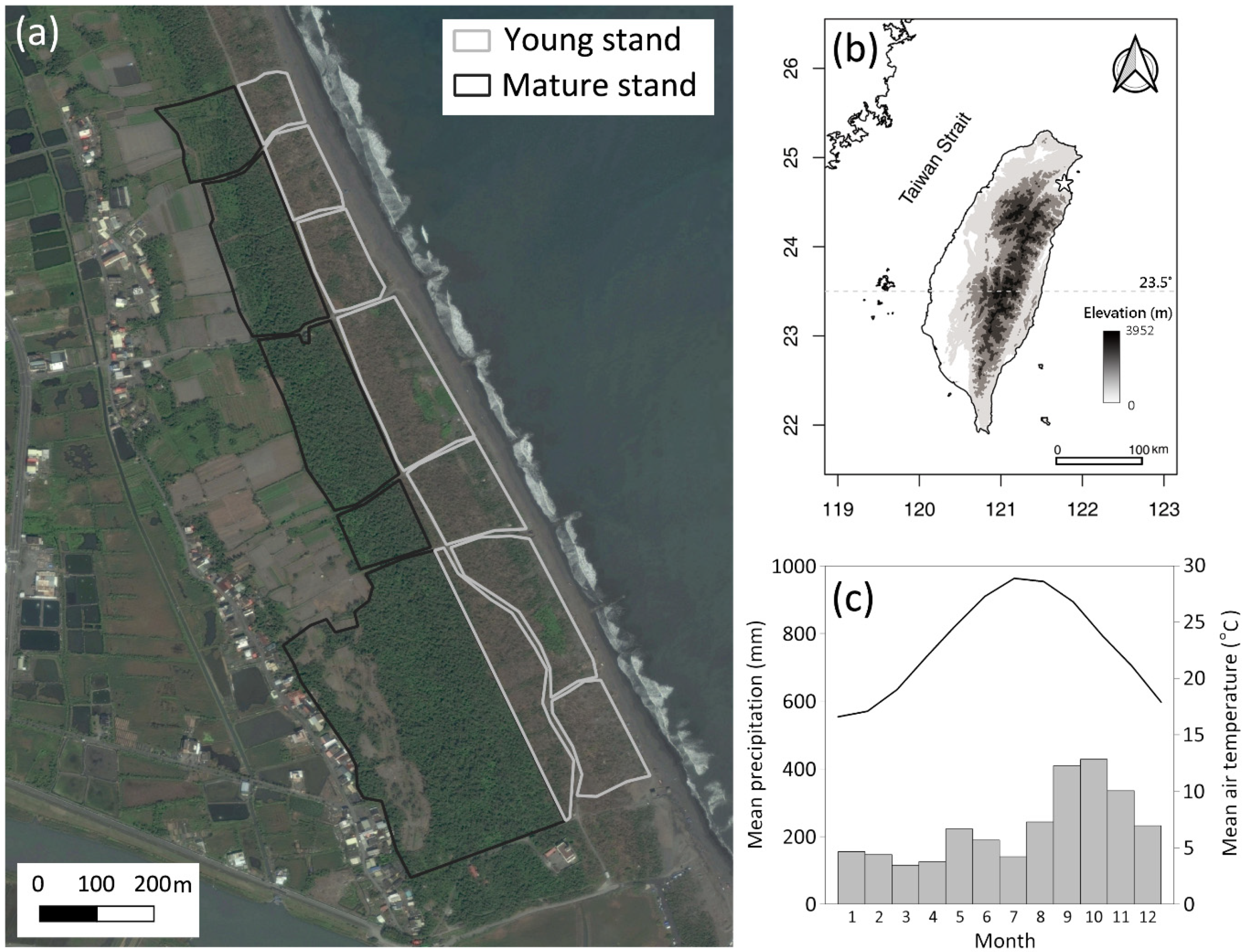
2.1. Study Site

In this study, we selected 60.7 ha of subtropical coastal broadleaf plantation forests located in northeastern Taiwan (24.727° N, 121.826° E) as our test sites for UAV canopy gap quantification (Figure 1). The areal size is relatively extensive by comparing with previous studies using similar tools [30,33,43,44]. The forests are dominated by Casuarina equisetifolia, Cerbera manghas, Terminalia catappa, Trema orientalis, Pongamia pinnata, Melaleuca leucadendra, Hibiscus tiliaceus and Pandanus odoratissimus. The young plantations (23.3 ha) were established after Typhoon Soudelor in 2015; more mature ones were established from 1975–1990 (37.4 ha). Most tree species within the study site are evergreen, without apparent seasonal defoliation. The mean tree diameter at breast height and height (±standard deviation (SD)) were 11.2 (±3.9) cm and 4.3 (±1.4) m, respectively, and tree density was 1167 tree ha−1 according to field survey conducted in 2020. The terrain is flat with elevation ranging from 5 to 16 m a.s.l. Long-term (1990–2021) mean annual precipitation and air temperature (±SD) of the site are 2744 (±309) mm y−1 and 22.8 (±4.5) °C, respectively, as determined by a local meteorological station (24.762° N, 121.748° E). The wet season (from August to December) receives 1649 mm y−1, which is about 85% of the annual precipitation (Figure 1c).

2.2. UAV Data Acquisition

UAVlidar and UAVphoto data were acquired on 20 July 2020 using a LiAir V scanning system (GreenValley International, Berkeley, CA, USA) and Sony α7 RII (Sony Group Corporation, Tokyo, Japan), respectively, carried by a Matrice M600 pro UAV (Da-Jiang Innovations, Shenzhen, China) at an altitude of 180 m a.g.l. The average point density was 11.2 points m−2. The UAV lidar first return and ground points were gridded with a spatial resolution of 1 m using adaptive kriging (SCOP++, Department of Geodesy and Geoinformation, Vienna, Austria) to generate the DSM and DTM, respectively. We then generated the CHM (CHMlidar) by subtracting the DTM (from UAVlidar) from the lidar DSM. For spatial continuity of the data, 80% forward and side overlaps were set before the flight [45]; the data were georegistered by referencing to nine ground control points using a handheld real-time kinematic (10 cm accuracy in the real-time kinematic (RTK) mode under the open-sky condition) global positioning system (GPS) (GeoXH, Trimble Inc., Sunnyvale, CA, USA). The UAVphoto data were acquired using 80% forward and side overlaps. Point-cloud data from the UAVphoto were interpolated and resampled to generate a 10 cm DSM using Pix4D (Pix4D SA, Lausanne, Switzerland). Mean x, y and z errors were established to be ≤3 cm by referring to the ground control points. The DSM derived from the UAVphoto was further aggregated to a 1 m spatial resolution by a nearest neighbor interpolation method using a geographical information system (QGIS v. 3.4.4, http://www.qgis.org, the last accessed date 28 April 2021), and the CHMphoto was also derived by subtracting the DTM from the DSM derived from the UAVphoto. Figure 2 shows the flowchart of the study.

2.3. Gap Detection

Gaps may be defined as canopy openings reaching within 2 m of the ground [15], with height thresholds being relative to the height of the canopy surrounding a gap. To determine canopy gaps, we defined a height class and took a horizontal cross-section of the CHM smaller than that height threshold, and then recorded agglomerations of empty pixels surrounded by the full pixels [46]. We repeated the analysis for a range of height thresholds up to the maximal canopy height with incremental 2 m intervals. We removed gap size < 5 m2 and >2 ha by referring to White et al. [6]. Finally, we applied both criteria on CHMlidar and CHMphoto. We note that the primary objective of this study is to only develop ideal toolsets for forest gap quantification. Therefore, only a standard gap delineation approach was applied in this study to make a reasonable comparison.
To assess gap detection performance, we randomly sampled 30 gaps each for young and mature stands (n = 60) in July 2021 by referring to both GAPlidar and GAPphoto, and georeferenced those gaps by using a handheld GPS. In addition, we estimated the size of each gap by referring to Runkle [47] and Yao et al. [19], assuming the shape of the gaps was elliptical, which should be appropriate for the application [48]. We then calculated the area (Equation (1)) by measuring the longest axis (L) and the one (W) perpendicular to L.
Gap area = πLW/4
We compared the size differences (e.g., root mean squared error (RMSE)) of field observation and GAPlidar and GAPphoto. We note that, to our knowledge, there were no disturbances (e.g., typhoons or forest management) between the times of UAV and field data acquisition. In addition, both the UAV and field campaigns were conducted in July. Therefore, the ramifications of the time difference between UAV and field sampling should be minimal.

2.4. Modeling Canopy Gap Distribution

We utilized the zeta and Weibull distributions to model the gap characteristics of coastal forests in the subtropical zone of northeastern Taiwan. The zeta distribution provides a summary of the frequency that is suitable for characterizing the distribution of landscape-level gap area [46,49] (Equation (2)):
f ( k ) = k λ ξ ( λ )
where the denominator is the Pareto distribution in a discrete power law probability density function. We employed the maximum likelihood to estimate λ for the zeta distribution [50]. The relationship (Equation (2)) becomes linear with a negative slope λ after transforming it to log–log space. The λ values usually vary from 1.0 to 3.0 for forests, and a greater value (e.g., >2) indicates more small gaps present in a forest (high-growth–low-mortality dynamics) and vice versa (mortality of large canopy) [4,36,51]. We derived λs for gaps derived from GAPlidar and GAPphoto. We calculated each area of the gap to have their canopy size and frequency, and then used derived parameters λ and k to fit a zeta distribution (Equation (2)) by referring to Asner et al. [4].
The Weibull distribution function has been commonly applied for fitting multishape distributions because of its flexibility in characterizing data profiles [52,53,54,55]. This function can also be used to model the probability of an increasing, decreasing or stable trend. The two-parameter Weibull distribution is suitable for modeling phenomena with a monotonic decrease trend, with its probability density function for gap size given by:
f ( g ) = β θ β g β 1 e x p ( g θ ) β ; θ ;   β > 0 ;   g > 0  
where f(g) is the decrease probability trend of gap size, and β and θ are the shape and scale parameters of the distribution with positive values. The β parameter, known as the shape parameter (the slope of the Weibull probability plot), determines the shape form of the Weibull family of distributions that best fits the data. The θ parameter is the characteristic gap size, which is also known as the scale parameter. We specifically studied Weibull p50 (p50 hereafter), the probability for which the gap size is the median of the Weibull probability density function. This metric was selected since p50 indicates that the median gap size is the area at which half of the amount is smaller than the median. Finally, we assessed the areal size effect of gap distribution quantifications for the zeta and Weibull distributions by randomly selecting 1–10 ha areas with a 1 ha increment for 30 times for the gaps (GAPlidar and GAPphoto) of young and mature forest stands and investigating the variation of λ and p50 (also termed the sensitivity analysis). We note that the descriptive statistics (e.g., mean, SD, median, min, max, skewness, kurtosis) were utilized to describe or summarize the characteristics of canopy gap data distribution. We applied the Shapiro–Wilk normality test (W) to investigate normality of the datasets. If the dataset was rejected by the Shapiro–Wilk test (not normally distributed), we then used Dunn’s test, which is a nonparametric pairwise multiple comparison procedure based on rank sums.

3. Results

3.1. Canopy Height Model Characteristics

The means (±SD) of young forest stand CHMs were 1.2 ± 0.9 m for CHMlidar and 1.4 ± 1.1 m for CHMphoto; those of mature forest stands were 4.0 ± 2.4 m for CHMlidar and 4.6 ± 2.2 m for CHMphoto (for examples, see Figure 3). None of the CHMs were normally distributed (p < 0.001) according to the Shapiro–Wilk normality test. According to Dunn’s test for multiple comparisons, a nonparametric pairwise multiple comparisons method [56], there were significant differences (p ≤ 0.001) of median CHMlidar and CHMphoto for both young and mature stands, but not for sensors of the same forest type (p = 0.97 and 0.58 for young and mature stands, respectively) (Table 1). In addition, Dunn’s test for multiple comparisons (Table 1) also demonstrated significant differences (p ≤ 0.001) of median CHMlidar and CHMphoto for both forest types but not for sensors of the same forest type (p ≥ 0.12).
Our field observation showed that 25 (16.7% not-gap rate with gap sizes ≤ 5 m2) and 26 (13.3% not-gap rate with gap sizes ≤ 5 m2) gaps were found in young and mature stands. The mean (±SD) of L in Equation (1) of young and mature stands was 15.2 ± 25.3 m and 17.3 ± 18.1 m, respectively; the mean (±SD) W of young and mature stands was 6.7 ± 12.6 m and 6.7 ± 6.5 m, respectively. With these parameters, we calculated the gap sizes for young (mean ± SD = 220.1 ± 915.3 m2) and mature (95.1 ± 402.1 m2) stands (Figure 4). Estimated errors (RMSE) were 145.2 m for GAPlidar and 256.2 m for GAPphoto for the young stands, and 87.2 m for GAPlidar and 218.5 m for GAPphoto for the old stands (Figure 5). There were strong agreements (R2 ≥ 0.94, p < 0.001) between ground and UAV measurements (Table 2), and the performance of UAVlidar was superior to UAVphoto.

3.2. Gap Characteristics

Total numbers of GAPlidar and GAPphoto derived from CHMlidar and CHMphoto varied markedly (n = 154 for GAPlidar and 128 for GAPphoto for young stands; n = 748 for GAPlidar and 165 for GAPphoto for mature stands) (Table 3). The mean (±SD) sizes of GAPlidar for young and mature stands were 1392.9 ± 4298.8 m2 and 74.0 ± 311.9 m2, respectively; GAPphoto for young and mature stands was 491.3 ± 1778.7 m2 and 65.9 ± 99.2 m2, respectively. Both GAPlidar and GAPphoto for young and mature stands were not normally distributed (p < 0.001, the Shapiro–Wilk normality test) (Table 3).

3.3. Zeta and Weibull Distributions

The results of zeta distribution for each dataset types were similar, and λs of GAPlidar for young and mature forest stands were 1.36 and 1.71, respectively; those of GAPphoto for young and mature forest stands were 1.45 and 1.61 (Figure 6), respectively. The results of fitted Weibull distributions depicted that the shape parameters of young stands were 0.3 for GAPlidar and 0.5 for GAPphoto, and the scale parameters were 426.3 m2 for GAPlidar and 181.4 m2 for GAPphoto. The shape parameters were 0.6 for GAPlidar and 0.9 for GAPphoto, and the scale parameters were 41.0 m2 for GAPlidar and 51.3 m2 for GAPphoto in mature stands (Table 4). In the young stands, the gap sizes of p50 were 185.7 m2 for GAPlidar and 85.4 m2 for GAPphoto. In the mature stands, the gap sizes of p50 were from 23.1 m2 for GAPlidar and 39.6 m2 for GAPphoto (Table 4).

3.4. Gap Size Distributions across Spatial Extents

To assess the influence of gap size distribution and the analyzed area, we changed the spatial extents from 1 to 10 ha with a 1 ha increment to detect gap characters by fitting the zeta and Weibull distributions. The locations of each spatial extent (1–10 ha) were randomly selected for 30 times. The values of λ were from 1.59 (1 ha) to 1.35 (10 ha) in young stands derived from GAPlidar, and from 1.84 (1 ha) to 1.41 (10 ha) in young stands derived from GAPphoto (Figure 7a). The analysis of zeta distribution show that λs were from 1.83 (1 ha) to 1.71 (10 ha) in mature stand derived from GAPlidar and from 1.95 (1 ha) to 1.71 (10 ha) in mature stands derived from GAPphoto (Figure 7b). In the young stands, the gap sizes of p50 were from 394.7 m2 (1 ha) to 185.4 m2 (10 ha) for GAPlidar, and from 259.6 m2 (1 ha) to 85.7 m2 (10 ha) for GAPphoto (Figure 7c). In the mature stands, the gap sizes of p50 were from 29.1 m2 (1 ha) to 23.3 m2 (10 ha) for GAPlidar, and from 40.5 m2 (1 ha) to 39.8 m2 (10 ha) for GAPphoto (Figure 7d).

4. Discussion

Canopy gap dynamics are pivotal metrics, which may indicate the conditions of forests from different perspectives including ecology, carbon sequestration and management. In this study, we verified that UAVlidar with the Weibull distribution may be an optimal approach to characterize canopy gaps of young and mature broadleaf plantation forests in a coastal region of northeastern Taiwan. To our knowledge, this UAVlidar gap analysis method has not been previously published. In this section, we deliberate the feasibility of using UAVlidar and UAVphoto to quantify canopy gaps, and demonstrate the applications on canopy gap monitoring with the availability of a proper analytical tool.

4.1. Canopy Gap Delineation Using UAVlidar and UAVphoto

The performance of remotely sensed canopy gap detection is sensitive to sensor types, such as high spatial resolution satellite optical imagery [57], point cloud data from airborne laser scanning [4,22] and terrestrial laser scanning [5]. In this study, we utilized UAVlidar and UAVphoto to quantify and analyze canopy gaps in coastal young and mature broadleaf forest plantations in the subtropical zone of northeast Taiwan. A pronounced discrepancy in the detection of the number of canopy gaps was discovered; a similar result was also observed in White et al. [6]. Both methods detected a similar number of canopy gaps in young forest stands, and UAVlidar observed 22.4% more gaps (n = 37) in 23.3 ha (Table 3). Since there was a strong agreement between field, GAPlidar and GAPphoto (Figure 5), we conclude that both UAVlidar and UAVphoto are suitable in detecting canopy gaps in young coastal broadleaf plantations.
On the other hand, UAVlidar can detect almost five times more gaps than UAVphoto (Table 3), especially for small gaps in mature forest stands. There was strong agreement between GAPlidar and field observation (RMSE = 87.2 m2), but not for GAPphoto (RMSE = 218.5 m2). This suggests that CHMphoto derived from UAVphoto using a standard approach may not be effective to map gaps in coastal mature broadleaf forests (also see [6]). The efficacy of UAVphoto is strongly related to the intensity of the ambient light in the visual region [58], which makes it challenging to delineate canopy gaps of certain UAVphoto view angles surrounded by shadow. Structure-from-motion (SfM) photogrammetry point-cloud-derived DSM for dense canopy might lead to a continuous surface between several tree canopies. Due to the presence of dense canopies in the mature forest plantations, the DSM from UAVphoto was unable to provide sufficient vertical points, while the DSM of UAVlidar did. Acquiring points in shaded canopy areas may be difficult for UAVphoto, which may significantly hinder its ability to detect small canopy gaps [6,59].
Lidar technology is known for being effective in delineating a multilayer canopy structure, especially for mature forests with dense canopies (23, 26) (Figure 3). In most cases, point cloud data acquired from UAVlidar were greater than those from airborne laser scanning (e.g., 10+ pts m−2 vs. 1–5 pts m−2) [43,44,60,61,62], making it an ideal tool for mapping gaps in dense forests. Although the UAVphoto is known to be cost effective for forest mapping [26] (in this case, costs for UAVlidar and UAVphoto were USD 7000 and 3000, respectively), it may not be feasible to delineate the vertical profile in coastal mature forests with dense canopies.

4.2. Canopy Gap Structure Status

Gap distribution may reflect the condition of a forest [63]; the power-law zeta distributions (λs) have a narrow range of values across different sites in forests [4,6,35,37]. In this study, we utilized λs to analyze GAPlidar and GAPphoto of young and mature coastal forest plantations. We found that λs fell into a narrow range (1.36–1.71) regardless of the forest types (Figure 6). According to the synthesis by Jucker [37], λs follow the same U-shaped pattern with canopy height and converge on relatively similar minimum values at multiple sites, therefore limiting the use of the zeta method in characterizing gap-size frequency distributions. These λs indicate that both young and mature forests were dominated by large gaps, perhaps due to high forest mortality [4]. This high mortality may be attributed to the periodic disturbance caused by summer tropical cyclones in the region (e.g., from June to October) [64]. This is also in agreement with Fisher et al. [36]. We also found that λs were insensitive to forest maturity (young vs. mature forest plantations) even with significant differences of GAPlidar and GAPphoto (Figure 6). The λ appears to converge on a narrow range of values across differences in forest structure, climate and disturbance history, which may limit its use for inferring the characteristics that shape the canopy structure dynamics of forests [37]. Therefore, we conclude that a power-law zeta distribution may not be feasible to monitor canopy gap variation of coastal plantation forests.
The other approach that we utilized to analyze canopy gaps was the Weibull distribution, forming the distributions of GAPlidar and GAPphoto with the shape and scale parameters (Table 4). The shape parameters were all <1 (an exponential distribution), ranging from 0.3 to 0.9 (Table 4), indicating the decreasing probability increasing with gap sizes [65]. Our result showed that a greater gap size (the young stands) may yield a small shape parameter. The values of the scale parameter derived from GAPlidar were greater than those of GAPphoto. In the young stands, the values of the Weibull distribution scale parameters derived from GAPlidar and GAPphoto were 426.3 and 181.4 m2, respectively; both indicate the presence of large gaps in the young broadleaf forest plantations. Therefore, the scale parameter may clearly distinguish the difference of GAPlidar and GAPphoto with the Weibull distribution.

4.3. Effects of Detected Areas

Stability of λs of power-law zeta distribution across spatial scales has been rarely investigated. In this study, we found that λs were stabilized after the spatial extent was >2 ha (3 ha) for both GAPlidar and GAPphoto in the young (mature) stands. In general, λs were more stable in the young stands than the mature ones due to the presence of several large gaps with relatively few small gaps (Figure 7a,b).
For the young stands, values of p50 GAPlidar consistently decreased until the spatial extent was ≥8 ha. On the other hand, those of GAPphoto stabilized when the spatial extents were ≥3 ha (Figure 7c). GAPlidar contained both small and large canopy gaps with greater variation (Table 3), as a consequence of high Weibull scale parameters through a range of spatial extents (Figure 7). Our results indicated that the domination numbers of gap size will affect the distribution, causing an increase of detected areas. The number of small gap size will result in the instability of p50. The method of UAVphoto is stabilized in small detected areas due to a lack of detection on the small gaps (Table 3), possibly due to the potential errors caused by shadow and data overlapping. Contrarily, UAVlidar was able to detect small canopy gaps and is therefore stabilized at a larger spatial extent. For mature stands, the values of p50 for both GAPlidar and GAPphoto were insensitive to spatial extents (Figure 7d), and UAVlidar was able to detect small canopy gaps for different spatial extents. The value of p50 was stabilized since small canopy gaps were dominant in mature forest stands. The results demonstrate that p50 may be applicable to assess characteristics of gaps in mature forest plantations regardless of spatial extents of the monitored region. Finally, on a side note, the sensitivity analysis (Figure 7) implies that the spatial extent (60.7 ha) of this study is sufficient for the application since all canopy gap metrics were stabilized before reaching the areal size of 10 ha.

5. Conclusions

This study assessed the feasibility of UAVlidar and UAVphoto to map canopy gaps of young and mature broadleaf plantation forests in a coastal region of northeastern Taiwan, and tested the feasibility of using different mathematical functions (power-law zeta and Weibull distributions) to characterize canopy gaps of forest stands. We found that both UAVlidar and UAVphoto may be able to quantify gaps in young plantations. However, only UAVlidar is able to thoroughly delineate gaps in mature plantations with a dense canopy layer. Lidar is able to detect small canopy gaps due to the physical nature of the instrument for better quantification of forest vertical profiles and insensitive to canopy shadow. By referring to the canopy gap analysis conducted in this study, we conclude that the Weibull distribution is a robust tool for coastal canopy gap monitoring. The proposed approach (UAVlidar with the Weibull distribution) may permit frequent monitoring of forest structure dynamics, which is particularly crucial in the era of climate change.

Author Contributions

Conceptualization, C.-H.C. and C.-y.H.; methodology, C.-H.C. and C.-y.H.; validation, C.-H.C.; formal analysis, C.-H.C.; investigation, C.-H.C. and C.-y.H.; resources, C.-H.C. and S.-L.D.; data curation, C.-H.C. and S.-L.D.; writing—original draft preparation, C.-H.C., J.W. and C.-y.H.; writing—review and editing, C.-H.C., J.W. and C.-y.H.; visualization, C.-H.C. and C.-y.H.; supervision, C.-y.H.; project administration, C.-H.C. and S.-L.D.; funding acquisition, C.-H.C. and C.-y.H. All authors have read and agreed to the published version of the manuscript.

Funding

This research was funded by the Ministry of Science and Technology (MOST) (110-2321-B-002-016-, 110-2321-B-004-001-), National Taiwan University (NTU-107L9010) and the Research Center for Future Earth, the Featured Areas Research Center Program, the Higher Education Sprout Project, and the Ministry of Education (MOE) in Taiwan.

Institutional Review Board Statement

Not applicable.

Informed Consent Statement

Not applicable.

Data Availability Statement

Not applicable.

Acknowledgments

We thank the editors for handling the manuscript, and the anonymous reviewers for providing suggestions that greatly improved the quality of the work.

Conflicts of Interest

The authors declare no conflict of interest.

References

  1. Denslow, J. Gap partitioning among tropical rainforest trees. Biotropica 1980, 12, 47–55. [Google Scholar] [CrossRef]
  2. Sommerfeld, R.A.; Lundquist, J.E.; Smith, J. Characterizing the canopy gap structure of a disturbed forest using the Fourier transform. For. Ecol. Manag. 2000, 128, 101–108. [Google Scholar] [CrossRef]
  3. Turner, M.G. Disturbance and landscape dynamics in a changing world. Ecology 2010, 91, 2833–2849. [Google Scholar] [CrossRef] [PubMed] [Green Version]
  4. Asner, G.P.; Kellner, J.R.; Kennedy-Bowdoin, T.; Knapp, D.E.; Anderson, C.; Martin, R.E. Forest canopy gap distributions in the southern Peruvian Amazon. PLoS ONE 2013, 8, e60875. [Google Scholar] [CrossRef] [Green Version]
  5. Seidel, D.; Ammer, C.; Puettmann, K. Describing forest canopy gaps efficiently, accurately, and objectively: New prospects through the use of terrestrial laser scanning. Agric. For. Meteorol. 2015, 213, 23–32. [Google Scholar] [CrossRef]
  6. White, J.C.; Tompalski, P.; Coops, N.C.; Wulder, M.A. Comparison of airborne laser scanning and digital stereo imagery for characterizing forest canopy gaps in coastal temperate rainforests. Remote Sens. Environ. 2018, 208, 1–14. [Google Scholar] [CrossRef]
  7. Mazdi, R.A.; Mataji, A.; Fallah, A. Canopy gap dynamics, disturbances, and natural regeneration patterns in a beechdominated Hyrcanian old-growth forest. Balt. For. 2021, 27, 535. [Google Scholar] [CrossRef]
  8. Sapkota, I.P.; Odén, P.C. Gap characteristics and their effects on regeneration, dominance and early growth of woody species. J. Plant Ecol. 2009, 2, 21–29. [Google Scholar] [CrossRef] [Green Version]
  9. Yamamoto, S.-I. Forest gap dynamics and tree regeneration. J. For. Res. 2000, 5, 223–229. [Google Scholar] [CrossRef]
  10. Panayotov, M.; Kulakowski, D.; Dos Santo, L.L.; Bebi, P. Wind disturbances shape old Norway spruce-dominated forest in Bulgaria. For. Ecol. Manag. 2011, 262, 470–481. [Google Scholar] [CrossRef]
  11. Gray, A.N.; Spies, T.A.; Pabst, R.J. Canopy gaps affect long-term patterns of tree growth and mortality in mature and old-growth forests in the Pacific Northwest. For. Ecol. Manag. 2012, 281, 111–120. [Google Scholar] [CrossRef]
  12. Attiwill, P.M. The disturbance of forest ecosystems: The ecological basis for conservative management. For. Ecol. Manag. 1994, 63, 247–300. [Google Scholar] [CrossRef]
  13. Kern, C.C.; Burton, J.I.; Raymond, P.; D’Amato, A.W.; Keeton, W.S.; Royo, A.A.; Walters, M.B.; Webster, C.R.; Willis, J.L. Challenges facing gap-based silviculture and possible solutions for mesic northern forests in North America. Forestry 2017, 90, 4–17. [Google Scholar] [CrossRef]
  14. Amiri, M.; Rahmani, R.; Sagheb-Talebi, K.H. Canopy gaps characteristics and structural dynamics in a natural unmanaged oriental beech (Fagus orientalis Lipsky) stand in the north of Iran. Casp. J. Environ. Sci. 2015, 13, 259–274. [Google Scholar]
  15. Brokaw, N.V. The definition of treefall gap and its effect on measures of forest dynamics. Biotropica 1982, 14, 158–160. [Google Scholar] [CrossRef]
  16. Clinton, B.D.; Baker, C.R. Catastrophic windthrow in the southern Appalachians: Charcteristics of pits and mounds and initial vegetation responses. For. Ecol. Manag. 2000, 126, 51–60. [Google Scholar] [CrossRef] [Green Version]
  17. Hart, J.L.; Grissino-Mayer, H.D. Gap-scale disturbance processes in secondary hardwood stands on the Cumberland Plateau, Tennessee, USA. Plant Ecol. 2009, 201, 131–146. [Google Scholar] [CrossRef]
  18. Kucbel, S.; Jaloviar, P.; Saniga, M.; Vencurik, J.; Klimas, V. Canopy gaps in an old-growth fir-beech forest remnant of Western Carpathians. Eur. J. For. Res. 2010, 129, 249–259. [Google Scholar] [CrossRef]
  19. Yao, A.-W.; Chiang, J.-M.; McEwan, R.; Lin, T.-C. The effect of typhoon-related defoliation on the ecology of gap dynamics in a subtropical rain forest of Taiwan. J. Veg. Sci. 2015, 26, 145–154. [Google Scholar] [CrossRef]
  20. Salvador-Van Eysenrode, D.; Bogaert, J.; Van Hecke, P.; Impens, I. Influence of tree-fall orientation on canopy gap shape in an Ecuadorian rain forest. J. Trop. Ecol. 1998, 14, 865–869. [Google Scholar] [CrossRef]
  21. Li, K.; Huang, X.; Zhang, J.; Sun, Z.; Huang, J.; Sun, C.; Xie, Q.; Song, W. A new method for forest canopy hemispherical photography segmentation based on deep learning. Forests 2020, 11, 1366. [Google Scholar] [CrossRef]
  22. Moura, Y.M.; Balzter, H.; Galvão, L.S.; Dalagnol, R.; Espírito-Santo, F.; Santos, E.G.; Garcia, M.; Bispo, P.d.C.; Oliveira, R.C.; Shimabukuro, Y.E. Carbon dynamics in a human-modified tropical forest: A case study using multi-temporal LiDAR data. Remote Sens. 2020, 12, 430. [Google Scholar] [CrossRef] [Green Version]
  23. Lefsky, M.A.; Cohen, W.B.; Parker, G.G.; Harding, D.J. Lidar remote sensing for ecosystem studies. BioScience 2002, 52, 19–30. [Google Scholar] [CrossRef]
  24. Saatchi, S.S.; Harris, N.L.; Brown, S.; Lefsky, M.; Mitchard, E.T.A.; Salas, W.; Zutta, B.R.; Buermann, W.; Lewis, S.L.; Hagen, S.; et al. Benchmark map of forest carbon stocks in tropical regions across three continents. Proc. Natl. Acad. Sci. USA 2011, 108, 9899–9904. [Google Scholar] [CrossRef] [PubMed] [Green Version]
  25. Lai, G.-Y.; Liu, H.-C.; Chung, C.-H.; Wang, C.-K.; Huang, C.-y. Lidar-derived environmental drivers of epiphytic bryophyte biomass in tropical montane cloud forests. Remote Sens. Environ. 2021, 253, 112166. [Google Scholar] [CrossRef]
  26. Chung, C.-H.; Wang, C.-H.; Hsieh, H.-C.; Huang, C.-y. Comparison of forest canopy height profiles in a mountainous region of Taiwan derived from airborne lidar and unmanned aerial vehicle imagery. GISci. Remote Sens. 2019, 56, 1289–1304. [Google Scholar] [CrossRef]
  27. Chung, C.-H.; Huang, C.-y. Hindcasting tree heights in tropical forests using time-series unmanned aerial vehicle imagery. Agric. For. Meteorol. 2020, 290, 108029. [Google Scholar] [CrossRef]
  28. Getzin, S.; Nuske, R.S.; Wiegand, K. Using Unmanned Aerial Vehicles (UAV) to Quantify Spatial Gap Patterns in Forests. Remote Sens. 2014, 6, 6988–7004. [Google Scholar] [CrossRef] [Green Version]
  29. Silva, C.A.; Valbuena, R.; Pinagé, E.R.; Mohan, M.; de Almeida, D.R.; North Broadbent, E.; Mohd Jaafar, W.S.W.; de Almeida Papa, D.; Cardil, A.; Klauberg, C. ForestGapR: An R package for forest gap analysis from canopy height models. Methods Ecol. Evol. 2019, 10, 1347–1356. [Google Scholar] [CrossRef] [Green Version]
  30. Kuželka, K.; Slavík, M.; Surový, P. Very High Density Point Clouds from UAV Laser Scanning for Automatic Tree Stem Detection and Direct Diameter Measurement. Remote Sens. 2020, 12, 1236. [Google Scholar] [CrossRef] [Green Version]
  31. Jaakkola, A.; Hyyppä, J.; Kukko, A.; Yu, X.; Kaartinen, H.; Lehtomäki, M.; Lin, Y. A low-cost multi-sensoral mobile mapping system and its feasibility for tree measurements. ISPRS J. Photogramm. Remote Sens. 2010, 65, 514–522. [Google Scholar] [CrossRef]
  32. Lin, Y.-C.; Cheng, Y.-T.; Zhou, T.; Ravi, R.; Hasheminasab, S.M.; Flatt, J.E.; Troy, C.; Habib, A. Evaluation of UAV LiDAR for mapping coastal environments. Remote Sens. 2019, 11, 2893. [Google Scholar] [CrossRef] [Green Version]
  33. Resop, J.P.; Lehmann, L.; Hession, W.C. Quantifying the Spatial Variability of Annual and Seasonal Changes in Riverscape Vegetation Using Drone Laser Scanning. Drones 2021, 5, 91. [Google Scholar] [CrossRef]
  34. Bonnet, S.; Gaulton, R.; Lehaire, F.; Lejeune, P. Canopy gap mapping from airborne laser scanning: An assessment of the positional and geometrical accuracy. Remote Sens. 2015, 7, 11267–11294. [Google Scholar] [CrossRef] [Green Version]
  35. Goulamoussène, Y.; Bedeau, C.; Descroix, L.; Linguet, L.; Hérault, B. Environmental control of natural gap size distribution in tropical forests. Biogeosciences 2017, 14, 353–364. [Google Scholar] [CrossRef] [Green Version]
  36. Fisher, J.I.; Hurtt, G.C.; Thomas, R.Q.; Chambers, J.Q. Clustered disturbances lead to bias in large-scale estimates based on forest sample plots. Ecol. Lett. 2008, 11, 554–563. [Google Scholar] [CrossRef]
  37. Jucker, T. Deciphering the fingerprint of disturbance on the three-dimensional structure of the world’s forests. New Phytol. 2022, 233, 612–617. [Google Scholar] [CrossRef]
  38. Weibull, W. Statistical theory of the strength of materials. Proc. Roy. Swedish Inst. Eng. Res. 1939, 151, 1–45. [Google Scholar]
  39. Weibull, W. Statistical distribution functions of wide applicability. J. Appl. Mech. 1951, 18, 293–297. [Google Scholar] [CrossRef]
  40. McCrum, W.R.; Sharp, J.T.; Bluhm, G.B. Use of the Weibull distribution for analysis of a clinical therapeutic study in rheumatoid arthritis. Henry Hosp. Med. J. 1976, 24, 173–182. [Google Scholar]
  41. Evans, J.; Kretschmann, D.; Green, D. Procedures for Estimation of Weibull Parameters; Gen. Tech. Rep. FPL-GTR-264; US Department of Agriculture, Forest Service, Forest Products Laboratory: Madison, WI, USA, 2019. [Google Scholar] [CrossRef]
  42. Phadnis, M.A.; Sharma, P.; Thewarapperuma, N.; Chalise, P. Assessing accuracy of Weibull shape parameter estimate from historical studies for subsequent sample size calculation in clinical trials with time-to-event outcome. Contemp. Clin. Trials Commun. 2020, 17, 100548. [Google Scholar] [CrossRef]
  43. Hu, T.; Sun, X.; Su, Y.; Guan, H.; Sun, Q.; Kelly, M.; Guo, Q. Development and Performance Evaluation of a Very Low-Cost UAV-Lidar System for Forestry Applications. Remote Sens. 2021, 13, 77. [Google Scholar] [CrossRef]
  44. Zhang, X.; Bao, Y.; Wang, D.; Xin, X.; Ding, L.; Xu, D.; Hou, L.; Shen, J. Using UAV LiDAR to Extract Vegetation Parameters of Inner Mongolian Grassland. Remote Sens. 2021, 13, 656. [Google Scholar] [CrossRef]
  45. Lisein, J.; Pierrot-Deseilligny, M.; Bonnet, S.; Lejeune, P. A Photogrammetric Workflow for the Creation of a Forest Canopy Height Model from Small Unmanned Aerial System Imagery. Forests 2013, 4, 922–944. [Google Scholar] [CrossRef] [Green Version]
  46. Kellner, J.R.; Asner, G.P. Convergent structural responses of tropical forests to diverse disturbance regimes. Ecol. Lett. 2009, 12, 887–897. [Google Scholar] [CrossRef]
  47. Runkle, J.R. Patterns of disturbance of disturbance in some old-growth mesic forests of eastern North America. Ecology 1982, 63, 1533–1546. [Google Scholar] [CrossRef] [Green Version]
  48. Hix, D.M.; Helfrich, K.K. Gap characteristics of southeastern Ohio second-growth forests. Gen. Tech. Rep. NC 1981, 234, 247–253. [Google Scholar]
  49. Marvin, D.C.; Asner, G.P.; Knapp, D.E.; Anderson, C.B.; Martin, R.E.; Sinca, F.; Tupayachi, R. Amazonian landscapes and the bias in field studies of forest structure and biomass. Proc. Natl. Acad. Sci. USA 2014, 111, E5224–E5232. [Google Scholar] [CrossRef] [Green Version]
  50. Hanel, R.; Corominas-Murtra, B.; Liu, B.; Thurner, S. Fitting power-laws in empirical data with estimators that work for all exponents. PLoS ONE 2017, 12, e0170920. [Google Scholar] [CrossRef] [Green Version]
  51. Lloyd, J.; Gloor, E.U.; Lewis, S.L. Are the dynamics of tropical forests dominated by large and rare disturbance events? Ecol. Lett. 2009, 12, 19–21. [Google Scholar] [CrossRef]
  52. Vose, J.M. Patterns of leaf area distribution within crowns of nitrogen-and phosphorus-fertilized loblolly pine trees. For. Sci. 1988, 34, 564–573. [Google Scholar]
  53. Maltamo, M.; Kangas, A.; Uuttera, J.; Torniainen, T.; Saramäki, J. Comparison of percentile based prediction methods and the Weibull distribution in describing the diameter distribution of heterogeneous Scots pine stands. For. Ecol. Manag. 2000, 133, 263–274. [Google Scholar] [CrossRef]
  54. Lovell, J.L.; Jupp, D.L.; Culvenor, D.S.; Coops, N.C. Using airborne and ground based ranging lidar to measure canopy structure in Australian forests. Can. J. Remote Sens. 2003, 29, 607–622. [Google Scholar] [CrossRef]
  55. Nijland, W.; Coops, N.C.; Macdonald, S.E.; Nielsen, S.E.; Bater, C.W.; Stadt, J.J. Comparing patterns in forest stand structure following variable harvests using airborne laser scanning data. For. Ecol. Manag. 2015, 354, 272–280. [Google Scholar] [CrossRef]
  56. Dinno, A. Nonparametric pairwise multiple comparisons in independent groups using Dunn’s test. Stata J. 2015, 15, 292–300. [Google Scholar] [CrossRef] [Green Version]
  57. Hobi, M.L.; Ginzler, C.; Commarmot, B.; Bugmann, H. Gap pattern of the largest primeval beech forest of Europe revealed by remote sensing. Ecosphere 2015, 6, 76. [Google Scholar] [CrossRef] [Green Version]
  58. Guimarães, N.; Pádua, L.; Marques, P.; Silva, N.; Peres, E.; Sousa, J.J. Forestry remote sensing from unmanned aerial vehicles: A review focusing on the data, Processing and Potentialities. Remote Sens. 2020, 12, 1046. [Google Scholar] [CrossRef] [Green Version]
  59. Vastaranta, M.; Wulder, M.A.; White, J.C.; Pekkarinen, A.; Tuominen, S.; Ginzler, C.; Kankare, V.; Holopainen, M.; Hyyppa, J.; Hyyppa, H. Airborne laser scanning and digital stereo imagery measures of forest structure: Comparative results and implications to forest mapping and inventory update. Can. J. Remote Sens. 2013, 39, 382–395. [Google Scholar] [CrossRef]
  60. Wallace, L.; Lucieer, A.; Malenovský, Z.; Turner, D.; Vopěnka, P. Assessment of forest structure using two UAV techniques: A comparison of airborne laser scanning and structure from motion (SfM) point clouds. Forests 2016, 7, 62. [Google Scholar] [CrossRef] [Green Version]
  61. Kellner, J.R.; Armston, J.; Birrer, M. New opportunities for forest remote sensing through ultra-high-density drone lidar. Surv. Geophys. 2019, 40, 959–977. [Google Scholar] [CrossRef] [Green Version]
  62. Jarron, L.R.; Coops, N.C.; MacKenzie, W.H.; Tompalski, P.; Dykstra, P. Detection of sub-canopy forest structure using airborne LiDAR. Remote Sens. Environ. 2020, 244, 111770. [Google Scholar] [CrossRef]
  63. Franklin, J.F.; Mitchell, R.J.; Palik, B.J. Natural Disturbance and Stand Development Principles for Ecological Forestry; Gen. Tech. Rep. NRS-19; US Department of Agriculture, Forest Service, Northern Research Station: Newtown Square, PA, USA, 2007. [Google Scholar] [CrossRef] [Green Version]
  64. Lin, T.-C.; Hamburg, S.P.; Lin, K.-C.; Wang, L.-J.; Chang, C.-T.; Hsia, Y.-J.; Vadeboncoeur, M.A.; Mabry McMullen, C.M.; Liu, C.-P. Typhoon disturbance and forest dynamics: Lessons from a northwest Pacific subtropical forest. Ecosystems 2011, 14, 127–143. [Google Scholar] [CrossRef]
  65. Dasgupta, R. Characterization theorems for Weibull distribution with applications. J. Environ. Stat. 2014, 6, 1–25. [Google Scholar]
Figure 1. (a) The study region, consisting of coastal young and mature broadleaf forest plantations (b) located in the subtropical region of northeast Taiwan (the star). The background image of (a) acquired in November 2015 was from Google Earth. (c) Monthly precipitation (gray-colored bars, the left y-axis) and air temperatures (the black line, the secondary y-axis) records of 1990–2021 for the study site during the observation period.
Remotesensing 14 00667 g001
Figure 2. The work flow of this study.
Remotesensing 14 00667 g002
Figure 3. An illustration of canopy gap detection. In this study, we utilized (a) CHMlidar and (b) CHMphoto to derived (c) GAPlidar and (d) GAPphoto, respectively.
Remotesensing 14 00667 g003
Figure 4. Ground gap size distributions of young stand (n = 25) and mature (n = 26) stands of the study site. The white dots, black rectangles and vertical black lines are medians, interquartile ranges and 1.5 × interquartile ranges, respectively.
Remotesensing 14 00667 g004
Figure 5. The comparison of ground (GAPground) and UAV (GAPUAV) lidar and UAV-photography-measured gap areas in mature and young coastal plantation forests.
Remotesensing 14 00667 g005
Figure 6. The summary of zeta distribution that provides the frequency characterizing the size distribution of (a) young and (b) mature stands derived from UAV lidar and air photographs.
Remotesensing 14 00667 g006
Figure 7. The exponent of zeta distributions (λs) for GAPlidar and GAPphoto in (a) young and (b) mature forest stands with different analyzed areas. The Weibull distributions of p50 for the scaled values of the distributions in (c) young and (d) mature stands that were derived from GAPlidar and GAPphoto.
Remotesensing 14 00667 g007
Table 1. Statistics of the canopy height model (CHM) derived using lidar (CHMlidar) and UAV photographs (CHMphoto) for mature and young stands in the study site. The abbreviations SD, Min and Max are standard deviation, minimum and maximum, respectively. Values with identical superscripts (“a” or “b”) indicate statistically insignificant (p > 0.05) differences by referring to Dunn’s test for multiple comparisons. All datasets were not normally distributed (p < 0.001) according to the Shapiro–Wilk normality test (W).
SensorForest TypeMeanSDMedianMinMaxSkewnessKurtosisW
CHMlidarYoung1.2 a0.90.6 a0.011.61.625.980.81
Mature4.0 b2.43.7 b0.016.80.683.380.97
CHMphotoYoung1.4 a1.11.1 a0.010.30.743.190.96
Mature4.6 b2.24.5 b0.017.50.213.160.99
Table 2. Comparisons (Figure 5) of ground and UAV observations (GAPground = b0 + b1 GAPsensor). All models are significant (p < 0.001).
SensorForest Typeb0b1R2
LidarYoung−26.410.920.99
Mature−4.410.940.97
PhotographYoung−15.120.850.97
Mature−65.080.750.94
Table 3. Summary gap detection results of comparison of canopy gap characteristics (GAPlidar and GAPphoto) derived from CHMlidar and CHMphoto. None of the datasets were normally distributed (p < 0.001) according to the Shapiro–Wilk normality test (W).
GAP TypeForest TypeGap NumberMean Gap Size (SD, m2)W
GAPlidarYoung1651392.9 (4298.8)0.18
Mature74874.0 (311.9)0.12
GAPphotoYoung128491.3 (1778.7)0.29
Mature15465.9 (99.2)0.57
Table 4. Summary of the fitted Weibull distributions of canopy gaps detected by UAV lidar and photographs. Note that p50 is the median of the Weibull probability density function (median gap size is the area at which half of the amount is smaller than the median).
SensorForest TypeWeibull Distribution Parameters
ShapeScalep50
LidarYoung0.3426.3185.7
LidarMature0.641.023.1
PhotographYoung0.5181.485.4
PhotographMature0.951.339.6
Publisher’s Note: MDPI stays neutral with regard to jurisdictional claims in published maps and institutional affiliations.

