Artificial Neural Network-Based Ionospheric Delay Correction Method for Satellite-Based Augmentation Systems

Abstract

Ionospheric delay is a critical error source in Global Navigation Satellite Systems (GNSSs) and a principal aspect of Satellite Based Augmentation System (SBAS) corrections. Grid Ionospheric Vertical Delays (GIVDs) are derived from the delays on Ionosphere Pierce Points (IPPs), which are observed by SBAS reference stations. SBAS master stations calculate ionospheric delay corrections by several methods, such as planar fit or Kriging. However, when there are not enough IPPs around an Ionosphere Grid Point (IGP) or the IPPs are unevenly distributed, the fitting accuracy of planar fit or Kriging is unsatisfactory. Moreover, the integrity bounds of Grid Ionospheric Vertical Errors (GIVEs) are overly conservative. Since Artificial Neural Networks (ANNs) are widely used in ionospheric research due to their self-adaptation, parallelism, non-linearity, robustness, and learnability, the ANN method for GIVD and GIVE derivation is proposed in this article. Networks are separately trained for IGPs, and five years of historical data are applied on network training. Principal Component Analysis (PCA) is applied for dimensionality reduction of geomagnetic and solar indices, which is employed as a network input feature. Furthermore, the GIVE algorithm of the ANN method is derived based on the distribution of the residual random variable. Finally, experiments are conducted on 12 IGPs over the East China region. Under normal ionospheric conditions, compared with the planar fit and Kriging methods, the residual reduction of the ANN method is approximately 15%. The ANN method fits the ionospheric delay residual error better. The percentage of GIVE availability under 2.7 m increases at least 25 points in comparison to Kriging. Under disturbed conditions, due to a lack of training samples, the ANN method is incompetent compared with planar fit or Kriging.

1. Introduction

Global Navigation Satellite System (GNSS)-based positioning services have been extensively used in Safety-of-Life (SoL) aeronautical applications, containing aircraft en route navigation, precision approach, and automatic landing. Nevertheless, the positioning performance of fundamental GNSS services is restricted by various error sources: satellite orbit error, satellite clock error, and ionospheric delay correction error, which make it unable to meet the requirements placed on accuracy, integrity, availability, and continuity of GNSSs for civil aviation users [1,2]. To this end, many countries and regions have established their Satellite-Based Augmentation System (SBAS) to provide GNSS users with additional differential correction information: satellite orbit correction, satellite clock correction, and ionospheric delay correction, and with integrity augmentation information: User Differential Range Error (UDRE) and Grid Ionospheric Vertical Error (GIVE) [3]. The Wide-Area Augmentation System (WAAS) has been fully operational since July 2003, providing SoL services for North and part of South America [4]. The Japanese Multi-functional Satellite Augmentation System (MSAS), European Geostationary Navigation Overlay Service (EGNOS), and Indian GPS-Aided GEO Augmented Navigation (GAGAN) were declared operational and certified for SoL services in 2007 [5], 2011 [6], and 2014 [5], respectively. Russia also finished their System for Differential Correction and Monitoring (SDCM) to provide augmentation for GPS and GLONASS [7]. SBASs under construction include the Korean Augmentation Satellite System (KASS) and Chinese BeiDou SBAS (BDSBAS) [5,8].

Since ionospheric delay is a critical error source in GNSSs, it is also a principal aspect of SBAS corrections. Unlike orbit and clock corrections provided for each satellite, ionospheric corrections are generated for each pre-defined geographical location with a resolution of 5° × 5°, known as the Ionosphere Grid Points (IGPs) [3,7,9]. IGPs located at an altitude of 350km in a thin shell over WGS 84 ellipsoid are widely adopted by SBASs [7,10,11]. The Message Type 18 (MT18) broadcast by SBAS GEO satellites contains IGP masks, while MT26 delivers Grid Ionospheric Vertical Delay (GIVD) and its confidence bound GIVE [2,11,12]. Several ionospheric associate analysis centers, IGS, CODE, UPC, JPL, ESA, CAS, produce and release the Global Ionospheric Maps (GIMs) [13]. Their post-processed final GIM products maintain high accuracy, which contributes references to ionospheric studies. However, final GIMs with a latency of 11 days is hard to fulfill the real-time demands of SBAS GIVD calculation. Actually, the SBAS estimates GIVDs utilizing vertical delays on Ionosphere Pierce Points (IPPs) observed by continuously operating reference stations. GIVE is essential integrity information of the SBAS that provides 99.9% confidence bounds of GIVD residuals [14]. Combined with UDRE, GIVE participates in determining the Protection Levels (PLs) of aviation users and further influences the availability of the Localizer Performance with Vertical guidance (LPV) service [15,16]. However, GIVE has a more complicated format than UDRE due to the variable ionospheric behavior [15].

The propagation delay of electromagnetic waves with fixed frequency passing through the ionosphere is proportional to route Total Electron Content (TEC). An appropriate method that demonstrates the spatial gradients and time correlations of TEC will provide high fitting accuracy. The Inverse Distance Weighting (IDW) grid method was one of the numerous ionospheric models conducted over the Continental United States (CONUS) when WAAS initiated [17,18]. The planar fit method was used during the WAAS Initial Operational Capability (IOC) version and also accepted by the Japanese MSAS as its ionospheric algorithm [18,19]. The Kriging method was presented by Sparks in 2011 and shown to outperform planar fit by 15% under disturbed ionospheric conditions [20]. Many other SBAS ionospheric methods were investigated for different geographical regions [18,21,22,23].

In virtue of their outstanding performance in integrating complex relationships and distributions, artificial intelligence and machine learning-based models are experiencing a boom in recent years. Accordingly, a series of research studies applying machine learning algorithms have been conducted to depict complicated spatial gradients and time correlations among ionospheric TEC distributions. Sabzehee [24], Inyurt [25], Tebabal [26], and Okoh [27] applied ANN-based methods for regional TEC modeling and prediction over Iran, Turkey, and Africa. Mallika et al. [28] applied the Principal Component Analysis (PCA) technique before an ANN to forecast ionospheric TEC. Zhang [29] and Kim [30] used Support Vector Machine (SVM)-based methods for regional ionospheric delay modeling and regional GIM expansion. Wen et al. [31] examined the performance of a TEC prediction model constructed by a Long Short-Term Memory (LSTM) neural network at different latitudes. The works introduced above focus on modeling the correlations between ionospheric features such as date, time, geographic coordinates, geomagnetic indices, solar activity indices, and local TEC applying machine learning-based models. However, machine learning methods for GIVD and GIVE are sparse. In this article, the ANN method for GIVD and GIVE is proposed. Specifically, it includes: designing and determining the network structure, activation function, loss function, optimizer and training strategy; completing feature selection and data pre-processing that affect the prediction effect of ANNs dramatically; proposing the integrity bound GIVE calculation algorithm for the ANN method.

An ANN consists of a large number of nodes arranged into multiple layers. Many classification and regression problems can be solved perfectly by ANNs, which act as nonlinear adaptive processing systems. Theoretically, a fully connected ANN with at least three layers can approach any continuous function as long as it is given sufficient hidden nodes. However, training small datasets on networks with excessive nodes and layers may cause overfitting problems. Since geomagnetic and solar indices are highly correlated, which will enhance the number of parameters and computational complexity, the PCA technique is applied. PCA is a multivariate statistical analysis method for data dimensionality reduction. It uses an orthogonal transformation to linearly project the observed data of a series of related variables into linearly uncorrelated variables, which are called Principal Components (PCs). One or several PCs that contribute the most to the data variation are sufficient to retain the information while others are abandoned.

The rest of the article is organized as follows. The next section introduces the experiment and data preparation. Then, planar fit, Kriging, and ANN methods for GIVD and GIVE derivation are elaborated in detail. Results of the ANN method under normal and disturbed ionospheric conditions are presented and compared with planar fit and Kriging. After that, the discussion is given. The last section summarizes the entire work and puts forward the prospect for further research.

2. Materials

2.1. Experimental Data

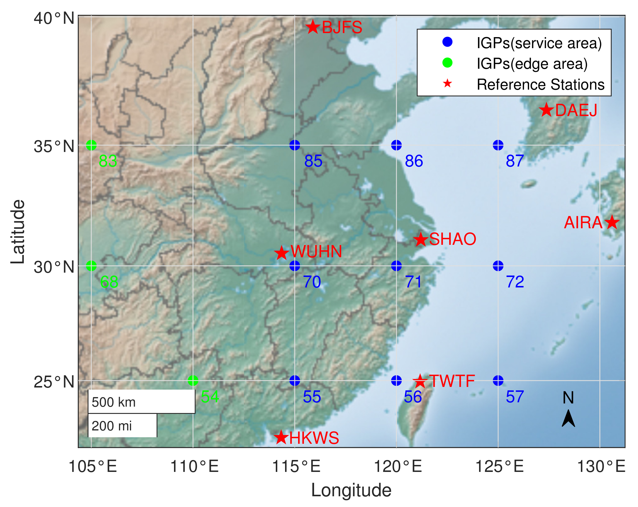
The BDSBAS service is an indispensable part of the BeiDou Navigation Satellite System (BDS); it is under construction and will provide single frequency service through a B1C signal for users in China and surrounding areas. Since the reference stations and experimental data are limited, twelve IGPs located in the East China region with dense airlines are selected to test the performance of the proposed method. Nine IGPs, 55 (25°N, 115°E), 56 (25°N, 120°E), 57 (25°N, 125°E), 70 (30°N, 115°E), 71 (30°N, 120°E), 72 (30°N,125°E), 85 (35°N,115°E), 86 (35°N, 120°E), 87 (35°N, 125°E), are situated within the reference station network region, and there are more than 30 IPPs for calculation. Three IGPs, 54 (25°N, 110°E), 68 (30°N, 105°E), 83 (35°N, 105°E), which are on the edge of the SBAS service area, represent IGPs with fewer than 30 IPPs. The surrounding IPP number of IGP 54 is slightly insufficient, the IPP number of IGP 68 is moderately insufficient, and the IPP number of IGP 83 is severely insufficient.

Seven stations from the International GNSS Service (IGS) are treated as SBAS reference stations in this research, namely, BJFS, WUHN, SHAO, HKWS, TWTF, DAEJ, AIRA. GPS constellation and observation data are employed. The distributions of experimental IGPs and reference stations are shown in Figure 1.

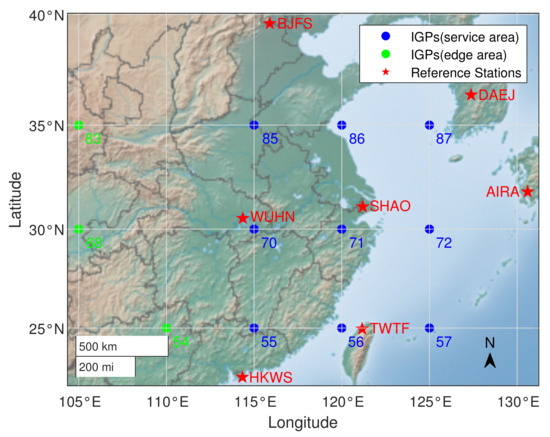
Figure 1. Distribution of selected experimental ionosphere grid points and SBAS reference stations. The region covers southeast China and part of the Western Pacific; five stations are located in China, one in Korea, and another one in Japan.

The ANN method requires reference stations to provide observation data of several years for training, however, there are few stations meeting the requirements in the China region. Therefore, the experimental stations and IGPs in this article are applied to verify the performance of the proposed method. Furthermore, the applicability of the ANN method has no limit in terms of application regions, and further study on the large regional span of China will be replicated when reference stations are available.

Center for Orbit Determination in Europe (CODE) final GIMs are picked as the reference IGP vertical delay, which was 11 days’ delay calculated with a Spherical Harmonic (SH) model. It is considered precise and used as a reference for many studies with 1-hour temporal resolution [13,30,32].

This study tested 3427 data points (23 per day at every hour except on 24 of 149 days) from January to May 2021, when the ionosphere was under normal conditions. The study also tested 44 data points (11 per day at every even hour except on 24 of 4 days) from 15 July 2012 and 17 March, 1 June, 29 June 2013, when the ionosphere was under disturbed conditions. Moreover, the ANN was trained and validated on 30,130 data points (23 per day at every hour except on 24 of 1310 days) from 2016 to 2020. Test, training, or validation data do not overlap on the timeline, which maintains the independence of the experiments. Figure 2 presents the Kp and Dst indices of selected days for training and testing. Table 1 shows the detailed data available by month.

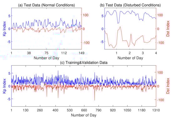
Figure 2. Geomagnetic indices Kp and Dst of the experimental data. (a) The daily average indices of test data under normal ionospheric conditions. (b) The hourly average indices of test data under disturbed ionospheric conditions. (c) The daily average indices of training and validation data.

Table 1. Data available in each month (in days). Test data under disturbed conditions are selected from 2012 and 2013; data from 2016 to 2020 are used to train and validate ANNs; test data under normal conditions are selected from 2021.

	January	February	March	April	May	June	July	August	September	October	November	December
2012	-	-	-	-	-	-	1	-	-	-	-	-
2013	-	-	1	-	-	2	-	-	-	-	-	-
2016	29	25	25	28	27	28	19	11	18	14	25	26
2017	8	-	3	9	29	29	31	31	27	27	28	31
2018	31	28	24	30	29	27	31	30	30	27	28	26
2019	30	28	18	-	-	-	-	-	-	-	-	-
2020	31	29	31	29	31	29	28	31	29	31	29	30
2021	30	28	30	30	31	-	-	-	-	-	-	-

2.2. Ipp Vertical Delay Extraction

The original Receiver Independent Exchange (RINEX) format data of seven reference stations are open access from the CDDIS website. To extract vertical delays of IPPs and their latitudes and longitudes, GPS observation files (O files) and navigation files (N files) are indispensable. Meanwhile, Differential Code Biases (DCBs) of satellites and stations are also needed; monthly satellite C1C(C1)-C1W(P1) and C1W(P1)-C2W(P2) DCBs are obtained from CODE; daily receiver C1-P2 DCBs are averaged from GNSS analysis centers’ Ionosphere Map Exchange (IONEX) files. Reference stations’ O files contain 30 s GPS observations of pseudocode C1, P2, and carrier phase L1C(L1), L2W(L2). For a fixed receiver, the observations are expressed as:

$$\left\{\begin{array}{c}{C}_1^i=R^i+I_1^i+T^i+c({\tau }^i-\tau )+D_1^i+D_1+E_{C_1}^i\\ P_2^i=R^i+I_2^i+T^i+c({\tau }^i-\tau )+D_2^i+D_2+E_{P_2}^i\end{array}\right.$$

(1)

$$\left\{\begin{array}{c}{L}_1^i=R^i-I_1^i+T^i+c({\tau }^i-\tau )-\lambda (B_1^i+N_1^i)+E_{L_1}^i\\ L_2^i=R^i-I_2^i+T^i+c({\tau }^i-\tau )-\lambda (B_2^i+N_2^i)+E_{L_2}^i\end{array}\right.$$

(2)

where $R^i$ is the true distance between the receiver and the i-th satellite antenna phase center; $I^i$ and $T^i$ are ionosphere and troposphere delays; c is the speed of light in vacuum; ${\tau }^i$ and $\tau$ are satellite and receiver clock errors; $D_j^i$ and $B_j^i$ represent the phase delays and advances caused by instrument biases of the i-th satellite at j-th frequency; $D_j$ represents the receiver hardware delay at j-th frequency; $\lambda$ and $N^i$ are wavelength and ambiguity of the carrier phase; $E^i$ terms are the residuals in the GPS measurements.

Taking the difference of dual-frequency code observations and carrier phase observations separately and neglecting the residuals, the results are shown as:

$$\left\{\begin{array}{c}{\Delta }_C^i=C_1^i-P_2^i=(I_1^i-I_2^i)+DC{B}^i+DCB\\ {\Delta }_L^i=L_1^i-L_2^i=-(I_1^i-I_2^i)-\lambda (B_1^i-B_2^i)-\lambda (N_1^i-N_2^i)\end{array}\right.$$

(3)

where $DC{B}^i=D_1^i-D_2^i$ and $DCB=D_1-D_2$ represent the satellite and receiver C1-P2 DCBs.

The pseudocode measurements are noisy but not ambiguous, while the carrier phase measurements are accurate but have cycle ambiguities. The Hatch filter is adopted to calculate the smoothed code measurements [33], and filtering process could be expressed as:

$${\Delta }_{C,Hatch}^i\left(k\right)=\frac{1}{K}{\Delta }_C^i\left(k\right)+\frac{K-1}{K}[{\Delta }_{C,Hatch}^i(k-1)+{\Delta }_L^i\left(k\right)-{\Delta }_L^i(k-1)]$$

(4)

where k is the epoch index and K = 12 (360 s) is the smoothing window width.

Before applying the Hatch filter, cycle-slips must be detected and removed from the data, or the cycle ambiguity terms $N^i$ in ${\Delta }_L^i$ will not cancel each other out between epochs. For a specific frequency, the ionospheric delay of electromagnetic waves could be expressed as a function of slant TEC:

$$I_1^i=\frac{40.28}{f_1^2}STEC;I_2^i=\frac{40.28}{f_2^2}STEC$$

(5)

Replacing ${\Delta }_C^i$ with the filtered ${\Delta }_{C,Hatch}^i$, and expressing the ionospheric delay terms as the above equations, we end up with the calculation equation of STEC:

$${\Delta }_{C,Hatch}^i=40.28(\frac{1}{f_1^2}-\frac{1}{f_2^2})STEC+DC{B}^i+DCB$$

(6)

RINEX N files help to calculate IPPs’ longitudes and latitudes at each epoch; meanwhile, the elevation angles of each satellite are known. Since the thin shell model is inaccurate for low elevation angle TEC estimation, IPP elevation angles less than 15° are abandoned. STECs of qualified IPPs are transferred to VTEC by multiplying an obliquity factor F:

$$VTEC=F·STEC;F={[1-{\left(\frac{Re·cos{A}^i}{Re+H}\right)}^2]}^{-\frac{1}{2}}$$

(7)

where $Re=6378.14$ km is the radius of the Earth, $H=350$ km is the height of the ionosphere thin shell, and $A^i$ is the elevation angle which has a cutoff value of 15°. Thus far, the geographic coordinates and vertical delays of IPPs at times corresponding to reference CODE GIMs are extracted from IGS RINEX files.

3. Methodology

In this section, three SBAS GIVD methods and their corresponding GIVE methods are interpreted in detail. The eligible IPPs are determined according to the IPP search algorithm for Kriging proposed by Sparks [20]. The target number of IPPs is 30, within a maximum fitting radius of 2100 km.

3.1. Planar Fit Method

All IPP locations participating in calculation need to be transferred from the Geodetic Coordinate System to the Earth-Centered, Earth-Fixed (ECEF) coordinate system. The transformation equation is given by:

$${\mathit{X}}_i=\left[\begin{array}{c}{x}_i\\ y_i\\ z_i\end{array}\right]=\left[\begin{array}{c}(Re+H)cos\left({\varphi }_i\right)cos\left({\lambda }_i\right)\\ (Re+H)cos\left({\varphi }_i\right)sin\left({\lambda }_i\right)\\ (Re+H)sin\left({\varphi }_i\right)\end{array}\right]$$

(8)

where ${\varphi }_i$ and ${\lambda }_i$ are, respectively, the latitude and longitude of IPPs.

The planar fit method is the most widely employed SBAS ionospheric delay method as a result of its outstanding performance and low computational cost. The ionosphere TEC dispersion could be described properly by a planar trend under normal conditions [19,20]. The estimated ionospheric delay plane (IGP as origin) contains three unknown coefficients and could be expressed as:

$$I(\Delta {\mathit{X}}_i)=a_0+a_1{\Delta {\mathit{X}}_i}^T·\widehat{\mathit{e}}+a_2{\Delta {\mathit{X}}_i}^T·\widehat{\mathit{n}}$$

(9)

where $\Delta {\mathit{X}}_i={\mathit{X}}_i-{\mathit{X}}_{IGP}$ is the distance separating the IPP from the IGP; $\widehat{\mathit{e}}$ and $\widehat{\mathit{n}}$ are, respectively, the unit vectors in east and north directions of the local Cartesian coordinate system whose origin is at the IGP, specified as follows:

$$\left\{\begin{array}{c}\widehat{\mathit{e}}={\left[\begin{array}{ccc}-sin\left({\lambda }_{IGP}\right)& cos\left({\lambda }_{IGP}\right)& 0\end{array}\right]}^T\\ \widehat{\mathit{n}}={\left[\begin{array}{ccc}-sin\left({\varphi }_{IGP}\right)cos\left({\lambda }_{IGP}\right)& -sin\left({\varphi }_{IGP}\right)sin\left({\lambda }_{IGP}\right)& cos\left({\varphi }_{IGP}\right)\end{array}\right]}^T\end{array}\right.$$

(10)

where ${\varphi }_{IGP}$ and ${\lambda }_{IGP}$ are the latitude and longitude of the IGP. The planar model coefficients $\left[\begin{array}{ccc}{a}_0& a_1& a_2\end{array}\right]$ are estimated by applying the least square fitting on the vertical delays at IPPs.

Before applying the least square fitting, the geometric matrix $\mathit{G}$ and the covariance matrix of the observations $\mathit{W}$ should be determined as follows:

$$\mathit{G}=\left[\begin{array}{ccc}1& {\Delta {\mathit{X}}_1}^T·\widehat{\mathit{e}}& {\Delta {\mathit{X}}_1}^T·\widehat{\mathit{n}}\\ 1& {\Delta {\mathit{X}}_2}^T·\widehat{\mathit{e}}& {\Delta {\mathit{X}}_2}^T·\widehat{\mathit{n}}\\ ⋮& ⋮& ⋮\\ 1& {\Delta {\mathit{X}}_N}^T·\widehat{\mathit{e}}& {\Delta {\mathit{X}}_N}^T·\widehat{\mathit{n}}\end{array}\right];\mathit{W}={\left[\begin{array}{cccc}{\sigma }_1^2+{\sigma }_{deco}^2& {\sigma }_{1,2}& \cdots & {\sigma }_{1,N}\\ {\sigma }_{1,2}& {\sigma }_2^2+{\sigma }_{deco}^2& \cdots & {\sigma }_{2,N}\\ ⋮& ⋮& \ddots & ⋮\\ {\sigma }_{1,N}& {\sigma }_{2,N}& \cdots & {\sigma }_N^2+{\sigma }_{deco}^2\end{array}\right]}^{-1}$$

(11)

where ${\sigma }_i$ denotes the variance of the ionosphere delay measurements at IPPs; ${\sigma }_{i,j}$ denotes the covariance between two IPP measurements caused by sharing the same satellite or receiver; ${\sigma }_{deco}=0.35$ m is the delay covariance associated with widely separated (uncorrelated) IPPs. $\mathit{I}={\left[\begin{array}{cccc}{I}_1& I_2& \cdots & I_N\end{array}\right]}^T$ represents the vertical delay vector of IPPs and, finally, the IGP vertical delay is estimated using the least square fitting as:

$$GIVD=a_0=\left[\begin{array}{ccc}1& 0& 0\end{array}\right]·\left[{\left({\mathit{G}}^T\mathit{W}\mathit{G}\right)}^{-1}{\mathit{G}}^T\mathit{W}\mathit{I}\right]$$

(12)

3.2. Kriging Method

The Kriging-based ionospheric method was introduced in the WAAS Follow-On Release 3 to replace the planar fit [20]. Kriging is a minimum mean square estimator which estimates the IGP delay by a weighted linear combination of IPP delays. The general equation of GIVD calculation applying Kriging is shown as:

$$GIVD=\sum _{i=1}^N{w}_i{I}_i={\mathit{w}}^T·\mathit{I}$$

(13)

where $\mathit{w}={\left[\begin{array}{cccc}{w}_1& w_2& \cdots & w_N\end{array}\right]}^T$ is the weight vector for IPPs. According to the methodology elucidated by Sparks, the weight vector is solved as a constrained optimization problem by the method of Lagrange multipliers. The solution of $\mathit{w}$ could be expressed as:

$$\mathit{w}=[\mathit{G}-{\mathit{W}}_{\mathit{K}}\mathit{G}{\left({\mathit{G}}^T{\mathit{W}}_{\mathit{K}}\mathit{G}\right)}^{-1}{\mathit{G}}^T{\mathit{W}}_{\mathit{K}}]\mathit{c}+{\mathit{W}}_{\mathit{K}}\mathit{G}{\left({\mathit{G}}^T{\mathit{W}}_{\mathit{K}}\mathit{G}\right)}^{-1}\mathit{s}$$

(14)

where $\mathit{s}=\left[\begin{array}{ccc}1& {\Delta \mathit{X}}^T·\widehat{\mathit{e}}& {\Delta \mathit{X}}^T·\widehat{\mathit{n}}\end{array}\right]$ is the distance indication vector, $\mathit{s}=\left[\begin{array}{ccc}1& 0& 0\end{array}\right]$ for IGP; ${\mathit{W}}_{\mathit{K}}={[\mathit{M}+\mathit{C}]}^{-1}$ is similar to the $\mathit{W}$ term in the planar fit method, moreover, Kriging describes the ionosphere decorrelation with a structure called the variogram.

The variogram results $\mathit{C}$ and $\mathit{c}$ are, respectively, an $N\times N$ matrix and $N\times 1$ vector, depicting the rate at which the values of a random function evaluated at two places become decorrelated as a function of their distance. $\mathit{M}$ is the measurement covariance matrix without considering decorrelation, i.e., $\mathit{M}={\mathit{W}}^{-1}-{\sigma }_{deco}^2·{\mathit{I}}_{N\times N}$, where ${\mathit{I}}_{N\times N}$ represents the identity matrix.

For ionosphere delay modeling, the observed behavior should be matched as a linear relation on separations close to the origin and a finite limit at infinity. Therefore, an exponential model is used for the variogram. The elements $C_{i,j}$ in $\mathit{C}$ and $c_i$ in $\mathit{c}$ are calculated by:

$$C_{i,j}=\left\{\begin{array}{cc}{\sigma }_{decototal}^2\hfill & i=j\hfill \\ ({\sigma }_{decototal}^2-{\sigma }_{deconomi}^2)exp(-\frac{D_{i,j}}{d_{deco}})\hfill & i\ne j\hfill \end{array}\right.$$

(15)

$$c_i=({\sigma }_{decototal}^2-{\sigma }_{deconomi}^2)exp(-\frac{d_i}{d_{deco}})$$

(16)

where ${\sigma }_{decototal}=0.65$ m, ${\sigma }_{deconomi}=0.3$ m, and $d_{deco}=8000$ km are, respectively, the delay covariance associated with uncorrelated IPPs, the delay covariance associated with nearly coincident IPPs, and the characteristic decorrelation distance; $D_{i,j}=\left|{\mathit{X}}_i-{\mathit{X}}_j\right|$ denotes the distance between the i-th IPP and j-th IPP, and $d_i=\left|{\mathit{X}}_i-{\mathit{X}}_{IGP}\right|$ is the distance from the i-th IPP to the IGP. In addition, when ${\sigma }_{decototal}$ and ${\sigma }_{deconomi}$ are set to be equal, the Kriging method downgrades to the planar fit.

3.3. GIVE Calculation for Planar Fit and Kriging

The Grid Ionospheric Vertical Error (GIVE) is critical information in the SBAS that ensures the integrity and availability of the system. GIVEs provide 99.9% confidence bounds on GIVD residuals [14]. As mentioned above, the planar fit method is a special case of the Kriging method. Thus, GIVE derivations for the planar fit and Kriging methods are similar.

GIVEs protect from the adverse influence of delay estimation, both sampled and undersampled [16]. The GIVE for the Kriging method is given by the following:

$$GIVE=K_{GIVE}\sqrt{{\sigma }_{IGP}^2+{\sigma }_{undersampled}^2}$$

(17)

where $K_{GIVE}=3.291$ is the constant that defines the 99.9% confidence interval, ${\sigma }_{IGP}^2$ corresponds to the variance of measurement error, modeling error, and sampling error of a relevant IGP. The composition of ${\sigma }_{IGP}^2$ is described by the following equation:

$${\sigma }_{IGP}^2=R_{irreg}^2({\mathit{w}}^T\mathit{C}\mathit{w}-2{\mathit{w}}^T\mathit{c}+{\sigma }_{decototal}^2)+{\mathit{w}}^T\mathit{M}\mathit{w}$$

(18)

where $R_{irreg}^2$ is an inflation factor for ionospheric and statistical uncertainty in chi-square statistics associated with the vertical delay estimation. Any calculated value of $R_{irreg}^2$ less than one is set to one. The inflation factor is computed by [14]:

$$R_{irreg}^2=MAX[{\chi }^2/{\chi }_{Pmd}^2\left(DoF\right),1]$$

(19)

${\chi }_{Pmd}^2\left(DoF\right)$ corresponds to the chi-square statistic value with degree of freedom $DoF$ in probability $Pmd$; the degree of freedom $DoF$ equals to the number of IPPs minus the number of parameters of the model; $Pmd$ is the probability of missed detection and is usually set to ${10}^{-3}$.

The accuracy of the vertical delay estimation will diminish as the ionospheric disturbance level increases. ${\chi }^2$ is introduced to inspect the goodness of fit, i.e., whether an estimation satisfies the accuracy requirement [20]. The detection strategy for ionospheric irregularities based on the chi-square is computed as the sum of the squares of the normalized residuals, written as follows:

$${\chi }^2={\mathit{I}}^T[{\mathit{W}}_{\mathit{K}}-{\mathit{W}}_{\mathit{K}}\mathit{G}{\left({\mathit{G}}^T{\mathit{W}}_{\mathit{K}}\mathit{G}\right)}^{-1}{\mathit{G}}^T{\mathit{W}}_{\mathit{K}}]\mathit{I}$$

(20)

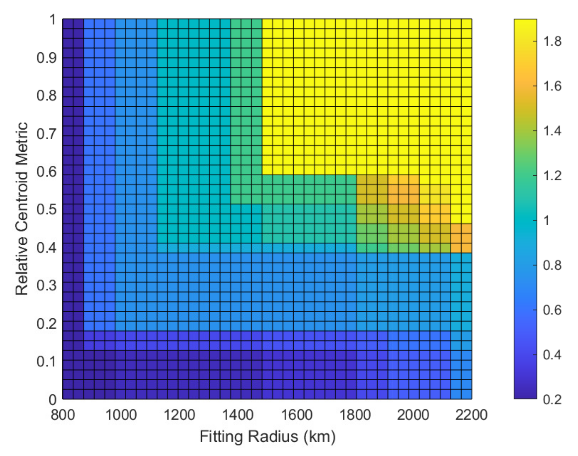
The SBAS also protects against estimation errors due to the undersampled irregularities of ionosphere TEC except for sampling errors. ${\sigma }_{undersampled}$ is known as the undersampled threat model. ${\sigma }_{undersampled}$ is both a function of the Relative Centroid Metric (RCM) and the fitting radius [15,34]. The RCM represents the ratio of the distance between the IPP centroid and the IGP to the fitting radius. The undersampled threat model applied in this paper is based on the WAAS release 8/9 model for planar fit and Kriging, and the model is shown in Figure 3 [16,34].

Figure 3. Undersampled threat model ${\sigma }_{undersampled}$ in meters.

By replacing ${\mathit{W}}_{\mathit{K}}$ with $\mathit{W}$, and setting ${\sigma }_{decototal}={\sigma }_{deconomi}={\sigma }_{deco}$, we could calculate GIVEs for the planar fit model following the same process.

3.4. ANN GIVD Method

Artificial Neural Networks (ANNs), also known as Multi-Layer Perceptrons (MLPs) or Back Propagation Networks (BPNs), are multilayer forward structured networks that consist of fully connected neurons. There is no necessity to determine the mathematical equation of the mapping relationship between inputs and outputs in advance. Only through the training process can ANNs learn the mapping rules and obtain the closest prediction to the expected result when new inputs are given. SBAS ionospheric delay modeling is a complex problem with abundant variations. Historical data assist ANNs in capturing such variations under different times, geographic locations, geomagnetic conditions, and solar conditions.

Next, the ANN method will be introduced in sections. Network structure and parameters, as well as its inputs and outputs, will be elaborated first. Then, the Principal Component Analysis (PCA) method for geomagnetic and solar index processing is presented. Finally, the network training strategy is described in detail.

3.4.1. Network Structure and Parameters

The finalized network is formatted to be a three-layer structure. It contains an input layer, a single hidden layer, and an output layer. There are 93 neurons in the input layer, which matches the number of inputs in each training and testing data point. There are 31 hidden neurons in the hidden layer, which is determined by considering the ratio of the training data size and the parameter size. The output layer has only one neuron, which outputs the vertical delay at the relevant IGP.

The ANN implemented in this article is fully connected. That is to say, there are connection weights between each neuron in the previous layer and all neurons in the next layer. Accordingly, the $93\times 31$ weight matrix ${\mathit{w}}_{\mathbf{1}}$ and $31\times 1$ weight vector ${\mathit{w}}_{\mathbf{2}}$ are formatted. In addition, after calculating the weighted sum at each neuron, a bias term is added to the result. Biases in the hidden layer are arranged in a $1\times 31$ vector ${\mathit{b}}_{\mathbf{1}}$, while the bias in the output layer is represented as ${\mathit{b}}_{\mathbf{2}}$. ${\mathit{w}}_{\mathbf{1}}$, ${\mathit{w}}_{\mathbf{2}}$, ${\mathit{b}}_{\mathbf{1}}$, and ${\mathit{b}}_{\mathbf{2}}$ are the network parameters to be learned through the training process.

The $1\times 93$ row vector ${\mathit{U}}_j$ denotes the j-th input vector of the network, $V_j$ is the corresponding output. An explicit introduction of typical three-layer neural network can be found in [25], and the network transfer function between inputs and outputs could be expressed as follows:

$$V_j=Sigmoid({\mathit{U}}_j{\mathit{w}}_{\mathbf{1}}+{\mathit{b}}_{\mathbf{1}}){\mathit{w}}_{\mathbf{2}}+{\mathit{b}}_{\mathbf{2}};Sigmoid\left(x\right)={(1+e^{-x})}^{-1}$$

(21)

Activation functions introduce nonlinear factors to the system and further enhance the expression ability of linear models. The sigmoid function is selected as the hidden layer activation function. As a pure nonlinear function, despite a risk of gradient disappearance and slower converging speed, sigmoid is convenient to take derivatives on GIVE calculations.

3.4.2. Network Inputs and Outputs

Three scalars and three vectors are stacked horizontally in the 93-dimensional input vector ${\mathit{U}}_j$. The formation of ${\mathit{U}}_j$ could be expressed in the following form:

$${\mathit{U}}_j=[{\alpha }_j,{\beta }_j,{\gamma }_j,{\mathsf{\Phi }}_j,{\mathsf{\Lambda }}_j,{\mathit{I}}_j]$$

(22)

where ${\alpha }_j$ is the modified day of year; ${\beta }_j$ is the modified time of day; ${\gamma }_j$ denotes the index of geomagnetic and solar conditions processed by PCA. ${\mathsf{\Phi }}_j$, ${\mathsf{\Lambda }}_j$, and ${\mathit{I}}_j$ are 30-dimensional row vectors, which represent the relative latitudes, the relative longitudes, and the ionospheric delays of 30 IPPs.

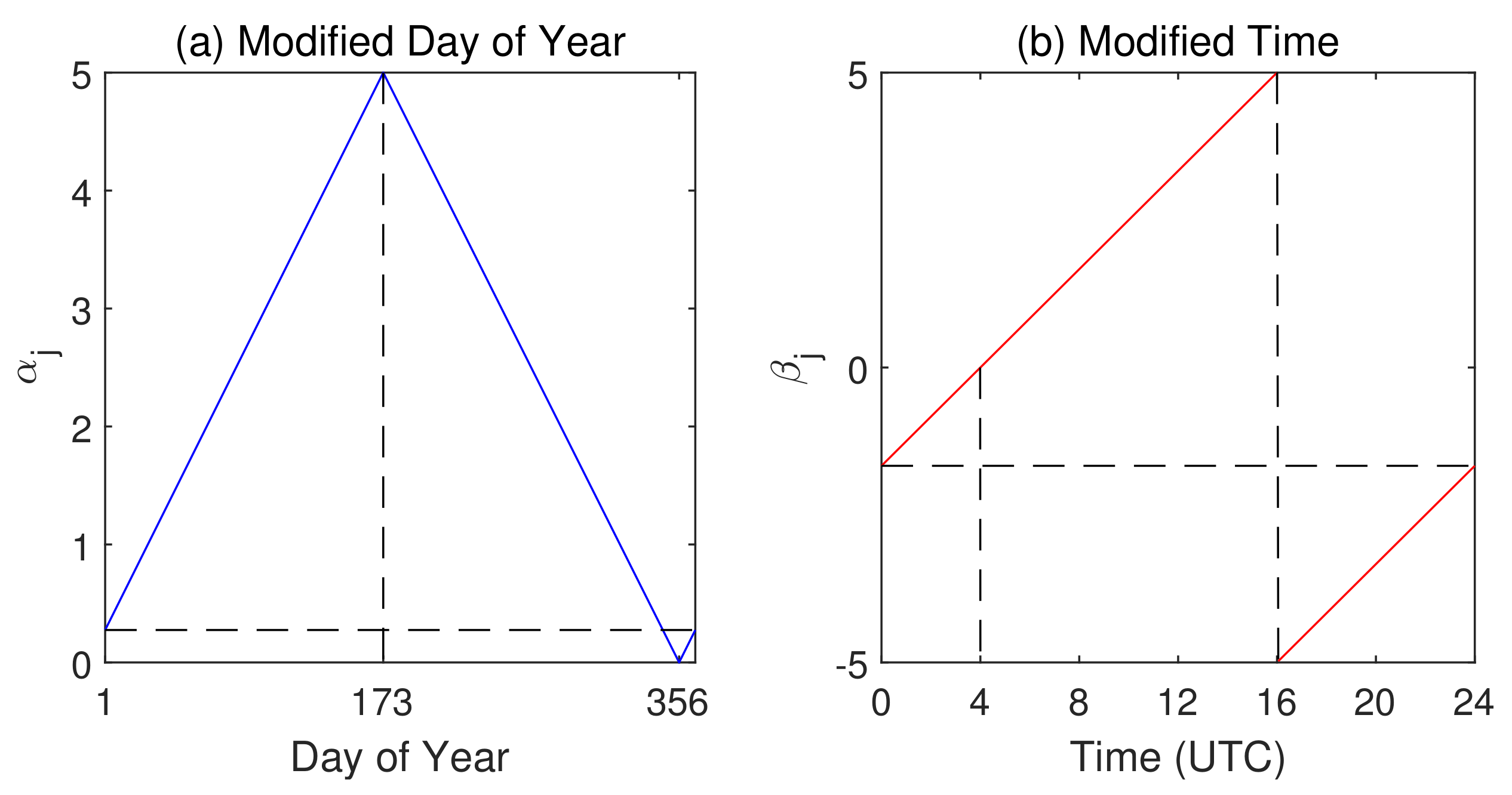
Considering that the sigmoid function has an apparent nonlinear interval between $-5$ and 5, all input features are scaled to this interval. Since the location of the subsolar point in the tropic affects the local ionosphere activity, day of year is chosen as an input feature. Similarly, the time of day also contains the subsolar point position information, and thus is also set as an input feature. However, directly using such day and time values is meaningless. They need to be modified to match the subsolar point locations. The modification function is shown in Figure 4.

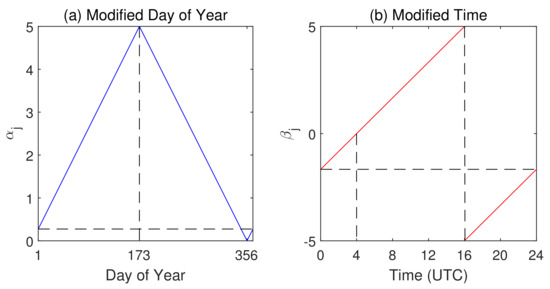
Figure 4. Modification function of feature ${\alpha }_j$ and ${\beta }_j$. (a) The variation in feature ${\alpha }_j$ as a function of day of year; peak appears on day 173 when subsolar point is on Tropic of Cancer; a trough on day 356 when subsolar point is on Tropic of Capricorn. (b) The mapping rule between UTC time and feature ${\beta }_j$; 4 o’clock UTC, when noon is at ${120}^{\circ }E$, is matched to zero; at 16 o’clock UTC, when midnight is at ${120}^{\circ }$, ${\beta }_j$ reaches peak and goes back to trough.

Components of ${\mathsf{\Phi }}_j$, ${\mathsf{\Lambda }}_j$, and ${\mathit{I}}_j$ are not required to be modified, they are scaled to the $-5$ to 5 interval by applying a min–max normalization method. The method could be expressed as the following equations:

$${\varphi }_{norm}=\frac{5\varphi }{{\left|\varphi \right|}_{max}};{\lambda }_{norm}=\frac{5\lambda }{{\left|\lambda \right|}_{max}};I_{norm}=\frac{5(2I-I_{max})}{I_{max}}$$

(23)

where $\varphi$, $\lambda$, and I denote the components of ${\mathsf{\Phi }}_j$, ${\mathsf{\Lambda }}_j$, and ${\mathit{I}}_j$; the parameters with subscript min and max represent the min and max values in the entire dataset. Since $\varphi$ and $\lambda$ represent latitude and longitude differences between IPP and IGP, they could be negative, and absolute values are used in the denominators. The details concerning ${\gamma }_j$ are introduced in the next subsection.

The 1-dimensional network output $V_j$ is the predicted ionospheric vertical delay at the relevant IGP, in other words, the predicted GIVD.

3.4.3. Principal Component Analysis

As mentioned before, geomagnetic and solar conditions also affect ionosphere TEC dramatically. Hence, geomagnetic indices Kp, Ap, and Dst, solar activity indices Sunspot Number (SSN), and solar radio flux 10.7 (F10.7) are taken into account when applying the ANN method. However, these five indices are highly correlated; when entirely set as network inputs, they will enhance the number of parameters and computational complexity. Thus, the PCA technique is applied to reduce the dimension of the indices from five to one and without missing major information.

${\gamma }_{\mathbf{org}}$ denotes the original geomagnetic and solar index matrix covering the total of 30,130 training and validation data points. The indices are Kp, Ap, Dst, SSN, and F10.7 collected from the OMNI data (spacecraft-interspersed, near-Earth solar wind data). The composition of ${\mathit{\gamma }}_{\mathit{org}}$ is shown as follows:

$${\mathit{\gamma }}_{\mathit{org}}=[\mathit{Kp},\mathit{Ap},\mathit{Dst},\mathit{SSN},\mathit{F}\mathbf{10}.\mathbf{7}]$$

(24)

where $\mathit{Kp}$, $\mathit{Ap}$, etc. are column vectors of the indices covering the entire training and validation data used for PCA fitting.

Data normalization is needed before calculating principal components, which means subtracting the column average from each element and dividing by the standard deviation. Taking the Kp column as an example, the normalization process could be expressed as the equations:

$$K{p}_{nor,j}=\frac{K{p}_j-mean\left(\mathit{Kp}\right)}{\sqrt{var\left(\mathit{Kp}\right)}};mean\left(\mathit{Kp}\right)=\frac{{\sum }_{j=1}^{30130}K{p}_j}{30130};var\left(\mathit{Kp}\right)=\frac{{\sum }_{j=1}^{30130}{[K{p}_j-mean\left(\mathit{Kp}\right)]}^2}{30130-1}$$

(25)

where $K{p}_{nor,j}$ and $K{p}_j$ are j-th components of normalized vector ${\mathit{Kp}}_{\mathit{nor}}$ and the original $\mathit{Kp}$. The other columns are operated similarly, and ${\mathit{\gamma }}_{\mathit{nor}}$ represents the indices matrix after all columns are normalized.

Since the data have been normalized, the $5\times 5$ sample correlation matrix ${\mathit{R}}_{\mathit{nor}}$ could be easily computed by the following equation:

$${\mathit{R}}_{\mathit{nor}}={\mathit{\gamma }}_{\mathit{nor}}^T{\mathit{\gamma }}_{\mathit{nor}}$$

(26)

the eigenvalue ${\lambda }_k$ reflects the contribution rate of the corresponding principal component to the integrity. By solving the characteristic equation of the sample correlation matrix ${\mathit{R}}_{\mathit{nor}}$, five eigenvalues are settled. Their corresponding eigenvectors ${\mathit{b}}_{\mathit{k}}$ are determined by solving each eigenvector equation. The calculation equations are shown in the following form:

$$\left|{\mathit{R}}_{\mathit{nor}}-{\lambda }_k{\mathit{I}}_{5\times 5}\right|=0;{\mathit{R}}_{\mathit{nor}}{\mathit{b}}_{\mathit{k}}-{\lambda }_k{\mathit{b}}_{\mathit{k}}=0$$

(27)

where || is to calculate the determinant of matrix; ${\mathit{I}}_{5\times 5}$ denotes the identity matrix. Reforming ${\lambda }_k$ in descending order and calculating the contribution rate of each eigenvalue as a percentage, we obtain 57.00%, 29.94%, 8.56%, 2.90%, and 1.60%.

In this article, the first principal component that keeps 57% of the information is selected as an input feature of the ANN (selecting more is also feasible). ${\lambda }_1$ and ${\mathit{b}}_{\mathbf{1}}$ represent the first eigenvalue and its corresponding eigenvector, feature ${\gamma }_j$ is the j-th component of feature vector $\gamma$. We obtain $\gamma$ from the following equation:

$$\mathit{\gamma }=\frac{5{\mathit{\gamma }}_{\mathit{nor}}{\mathit{b}}_{\mathbf{1}}}{{\left|{\mathit{\gamma }}_{\mathit{nor}}{\mathit{b}}_{\mathbf{1}}\right|}_{max}}$$

(28)

where the denominator means calculating the maximum absolute value in vector ${\mathit{\gamma }}_{\mathit{nor}}{\mathit{b}}_{\mathbf{1}}$. Testing or real-time data are also transformed by applying the fitted PCA parameters, i.e., mean, variance, and eigenvector. By applying PCA, the input dimensions are reduced substantially, while the primary information is retained.

3.4.4. Training Strategy

In the previous subsections, each element of input vector ${\mathit{U}}_j$ is elaborated. The entire dataset $\mathit{U}$ with dimension 33,601 $\times 93$ is separated into a 30,130 $\times 93$ training and validation matrix ${\mathit{U}}_{train/valid}$, a $3427\times 93$ testing matrix under normal conditions ${\mathit{U}}_{ntest}$, and a $44\times 93$ testing matrix under disturbed conditions ${\mathit{U}}_{dtest}$. The splitting specific of each partition is introduced in Section 2.1. Moreover, considering the data volume and splitting strategy adopted by other works [25,32], ${\mathit{U}}_{train/valid}$ is randomly split into the training data ${\mathit{U}}_{train}$ and the validation data ${\mathit{U}}_{valid}$ in the ratio $8:1$. ${\mathit{Y}}_{train}$, ${\mathit{Y}}_{valid}$, ${\mathit{Y}}_{ntest}$, and ${\mathit{Y}}_{dtest}$ are the corresponding reference IGP vertical delay vectors.

Training data are the data that contribute and determine the network parameters through the training process; validation data are used to evaluate the training performance and to avoid overfitting problems, while test data are the simulation of real-time data that test the fitting effect of the ANN model.

Before training, the loss function needs to be defined. Loss function pertains to the error to be minimized. In this article, the Mean Absolute Error (MAE) is set to be the loss function and calculated as follows:

$$L=\frac{1}{batch}\sum _{j=1}^{batch}\left|V_j-Y_j\right|$$

(29)

where $V_j$, which is mentioned in Equation (21), represents the j-th output of the network, and $Y_j$ is the corresponding reference. $batch$ represents the batch size in each iteration. As long as GPU memory is available, batch size could be set to the dimension of the entire training data, i.e., $batch=$ 26,703.

The training strategy incorporates a feed forward propagation process that determines the loss, an error backpropagation process that calculates the gradients and updates the parameters, and iteration of the above. In order to minimize the loss, each component in the network parameter matrices and vectors ${\mathit{w}}_{\mathbf{1}}$, ${\mathit{w}}_{\mathbf{2}}$, ${\mathit{b}}_{\mathbf{1}}$,and ${\mathit{b}}_{\mathbf{2}}$ has to be modified towards its negative gradient. The gradient is calculated by taking the partial derivative of the loss function with respect to the relevant parameter.

The Adam optimizer is applied to update parameters and minimize loss [35]. Adam is derived from the adaptive moment estimation, it is a variant of the gradient descent algorithm. The learning rate of each parameter is dynamically adjusted by using the first and second order moment estimation of the gradient, which keeps the parameters stable. The parameter update rule of the Adam optimizer could be expressed as:

$$w_{t+1}=w_t-\frac{lr·{\widehat{u}}_{t+1}}{(\sqrt{{\widehat{v}}_{t+1}}+ϵ)}$$

(30)

$${\widehat{u}}_{t+1}=\frac{{\beta }_1·u_t+(1-{\beta }_1)·g_{t+1}}{1-{\beta }_1^{t+1}};{\widehat{v}}_{t+1}=\frac{{\beta }_2·u_t+(1-{\beta }_2)·g_{t+1}^2}{1-{\beta }_2^{t+1}}$$

(31)

$$u_t={\beta }_1·u_{t-1}+(1-{\beta }_1)·g_t;v_t={\beta }_2·u_{t-1}+(1-{\beta }_2)·g_t^2$$

(32)

where t is the epoch index; $u_t$ and ${\widehat{u}}_{t+1}$ are, respectively, biased and corrected first moments; $v_t$ and ${\widehat{v}}_{t+1}$ are biased and corrected second raw moments; $g_t$ denotes the gradient at the $t^{th}$ epoch; $lr=0.001$ is the learning rate; ${\beta }_1=0.9$ and ${\beta }_2=0.999$ are exponential decay rates; $ϵ={10}^{-8}$ is constant to avoid a zero denominator.

Validation data ${\mathit{U}}_{valid}$ and their corresponding reference ${\mathit{Y}}_{valid}$ are used to evaluate the training performance, they detect overfitting and help to decide the training epoch number. Epoch is the number of iterations of parameter updates before training stops, it is usually set on when the validation loss starts to rise.

When the training process finishes, all epochs and parameter matrices ${\mathit{w}}_{\mathbf{1}}$, ${\mathit{w}}_{\mathbf{2}}$, ${\mathit{b}}_{\mathbf{1}}$, and ${\mathit{b}}_{\mathbf{2}}$ (containing 2946 parameters) are determined and recorded. With ${\mathit{U}}_{ntest}$, ${\mathit{U}}_{dtest}$, or real-time data passing through, the network outputs the predicted IGP vertical delay results, i.e., GIVD.

3.5. GIVE Calculation for ANN Method

When the training process of an ANN is completed, the nonlinear model will have a fixed relationship between its inputs and output. We use a generalized function $\mathit{f}({\mathit{U}}_j,\mathit{P})$ to represent this relationship and give the following equations:

$$V_j=Sigmoid({\mathit{U}}_j{\mathit{w}}_{\mathbf{1}}+{\mathit{b}}_{\mathbf{1}}){\mathit{w}}_{\mathbf{2}}+{\mathit{b}}_{\mathbf{2}}=\mathit{f}({\mathit{U}}_j,\mathit{P});\mathit{P}=\{{\mathit{w}}_{\mathbf{1}},{\mathit{w}}_{\mathbf{2}},{\mathit{b}}_{\mathbf{1}},{\mathbf{b}}_{\mathbf{2}}\}$$

(33)

where $\mathit{P}$ is the set that contains all network parameters. If ${\mathit{P}}^{*}$ represents the true parameter set for the function which models the system, there only exists a Gaussian random error $ϵ$ between network prediction and the reference:

$$Y_j=\mathit{f}({\mathit{U}}_j,{\mathit{P}}^{*})+{ϵ}_j$$

(34)

where each ${ϵ}_j$ is an independently and identically distributed Gaussian random variable with zero mean and variance ${\sigma }^2$. We minimize the loss function L and derive $\mathit{P}$ as a good estimation of ${\mathit{P}}^{*}$ by applying the error backpropagation algorithm in the training process. Hence, $\mathit{P}$ is very close to the true values ${\mathit{P}}^{*}$, and a Taylor expansion to the first order could be used to approximate $\mathit{f}({\mathit{U}}_j,\mathit{P})$ in terms of $\mathit{f}({\mathit{U}}_j,{\mathit{P}}^{*})$:

$$\mathit{f}({\mathit{U}}_j,\mathit{P})=\mathit{f}({\mathit{U}}_j,{\mathit{P}}^{*})+{\mathit{\delta }}_{\mathit{j}}^T(\mathit{P}-{\mathit{P}}^{*});{\mathit{\delta }}_{\mathit{j}}^T=[\frac{\partial \mathit{f}({\mathit{U}}_j,{\mathit{P}}^{*})}{\partial P_1^{*}},\frac{\partial \mathit{f}({\mathit{U}}_j,{\mathit{P}}^{*})}{\partial P_2^{*}},\cdots ,\frac{\partial \mathit{f}({\mathit{U}}_j,{\mathit{P}}^{*})}{\partial P_p^{*}}]$$

(35)

The prediction residual is defined by $Y_j-V_j$, and given Equations (33)–(35), the ionospheric delay residuals could be expressed as:

$$Y_j-V_j=Y_j-\mathit{f}({\mathit{U}}_j,{\mathit{P}}^{*})-{\mathit{\delta }}_{\mathit{j}}^T(\mathit{P}-{\mathit{P}}^{*})={ϵ}_j-{\mathit{\delta }}_{\mathit{j}}^T(\mathit{P}-{\mathit{P}}^{*})$$

(36)

To derive the integrity bound, the expected value, as well as the variance of the residual random variable, needs to be calculated by applying the following equations:

$$\left\{\begin{array}{c}E[Y_j-V_j]=E\left[{ϵ}_j\right]-{\mathit{\delta }}_{\mathit{j}}^{T}E\left[(\mathit{P}-{\mathit{P}}^{*})\right]\\ Var[Y_j-V_j]=Var\left[{ϵ}_j\right]+{\mathit{\delta }}_{\mathit{j}}^{T}Var\left[(\mathit{P}-{\mathit{P}}^{*})\right]{\mathit{\delta }}_{\mathit{j}}\end{array}\right.$$

(37)

Since there is statistical independence between random variables ${ϵ}_j$ and $\mathit{P}$, they are decoupled in calculating expectation and variance. Rivals and Personnaz discussed the distribution of $\mathit{P}-{\mathit{P}}^{*}$ in detail for neural networks. $\mathit{P}-{\mathit{P}}^{*}$ is also a Gaussian random variable with zero mean and variance ${\sigma }^2{({\Delta }^T\Delta )}^{-1}$ [36]. $\Delta$ denotes the Jacobian matrix of the training data (and/or validation data) with respect to the parameters, and has the following form:

$$\Delta =\left[\begin{array}{cccc}\frac{\partial \mathit{f}({\mathit{U}}_1,{\mathit{P}}^{*})}{\partial P_1^{*}}& \frac{\partial \mathit{f}({\mathit{U}}_1,{\mathit{P}}^{*})}{\partial P_2^{*}}& \cdots & \frac{\partial \mathit{f}({\mathit{U}}_1,{\mathit{P}}^{*})}{\partial P_p^{*}}\\ \frac{\partial \mathit{f}({\mathit{U}}_2,{\mathit{P}}^{*})}{\partial P_1^{*}}& \frac{\partial \mathit{f}({\mathit{U}}_2,{\mathit{P}}^{*})}{\partial P_2^{*}}& \cdots & \frac{\partial \mathit{f}({\mathit{U}}_2,{\mathit{P}}^{*})}{\partial P_p^{*}}\\ ⋮& ⋮& \ddots & ⋮\\ \frac{\partial \mathit{f}({\mathit{U}}_n,{\mathit{P}}^{*})}{\partial P_1^{*}}& \frac{\partial \mathit{f}({\mathit{U}}_n,{\mathit{P}}^{*})}{\partial P_2^{*}}& \cdots & \frac{\partial \mathit{f}({\mathit{U}}_n,{\mathit{P}}^{*})}{\partial P_p^{*}}\end{array}\right]$$

(38)

where n and p are data point number of the training (and/or validation) set and parameter number of the network. For the well-trained network with a large amount of data, each parameter in $\mathit{P}$ is within a small neighborhood of the corresponding element in ${\mathit{P}}^{*}$. Therefore, we could replace ${\mathit{P}}^{*}$ with $\mathit{P}$ in partial derivative calculations.

Moreover, $\mathit{P}$ is also regarded as an approximation of ${\mathit{P}}^{*}$ in calculating the unbiased estimation of ${\sigma }^2$:

$${\sigma }^2=\frac{{∥{\mathit{Y}}_{train}-\mathit{f}({\mathit{U}}_{train},\mathit{P})∥}^2}{n-p}$$

(39)

If the validation data ${\mathit{Y}}_{valid}$ and ${\mathit{U}}_{valid}$ are used to estimate ${\sigma }^2$, the parameter DoF p does not need to be subtracted from n in the denominator.

To sum up, the prediction residual of the ANN is also a Gaussian random variable with zero mean and variance ${\sigma }^2+{\sigma }^2{\mathit{\delta }}_{\mathit{j}}^T{({\Delta }^T\Delta )}^{-1}{\mathit{\delta }}_{\mathit{j}}$. GIVE for the neural network GIVD method is derived from the following equation:

$$GIV{E}_j=t_{n-p}^{\alpha /2}\sqrt{{\sigma }^2+{\sigma }^2{\mathit{\delta }}_{\mathit{j}}^T{({\Delta }^T\Delta )}^{-1}{\mathit{\delta }}_{\mathit{j}}}$$

(40)

where $t_{n-p}^{\alpha /2}$ is the t-distribution inflation factor that gives the $(1-\alpha )\times 100\%$ confidence bound for the predicted GIVD. $t_{n-p}^{\alpha /2}=t_{\infty }^{0.0005}=3.291$ for a $99.9\%$ integrity level.

Since the planar fit and Kriging methods apply empirical models, the GIVE derivation has to independently consider various threat factors for safety-critical purposes. In contrast, the ANN method derives GIVEs based on modeling of the residual random variable and statistical analysis of historical data. Therefore, the error sources and threat factors are integrally considered in the GIVE method. Specifically, the measurement errors of station receivers are contained in the ${\sigma }^2$ term, and the data points that have large decorrelation or undersampled threat will provide large gradients to the network parameter vector and are further reflected by the ${\mathit{\delta }}_{\mathit{j}}^T{({\Delta }^T\Delta )}^{-1}{\mathit{\delta }}_{\mathit{j}}$ term in Equation (40).

4. Results

Experiments are conducted on an Intel i5-10400F CPU and Nvidia 1050Ti GPU. The software environment is based on Python 3.7.4 and TensorFlow 2.4.1. The training process is operated on 26,703 pairs of training data ${\mathit{U}}_{train}$, ${\mathit{Y}}_{train}$ and validated on 3427 pairs of validation data ${\mathit{U}}_{valid}$, ${\mathit{Y}}_{valid}$, which are approximately in a ratio of 8:1. The training process lasts 72 s.

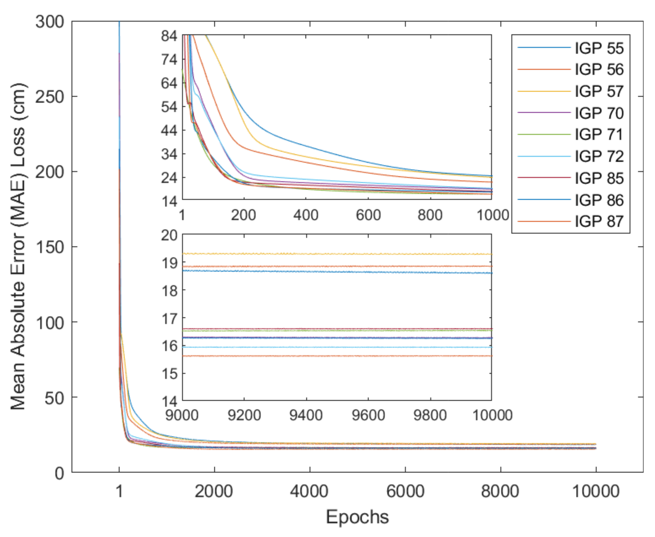
Different from the planar fit and Kriging methods, neural network models are trained for each IGP shown in Figure 1. Figure 5 shows the decay of validation loss along with training epochs.

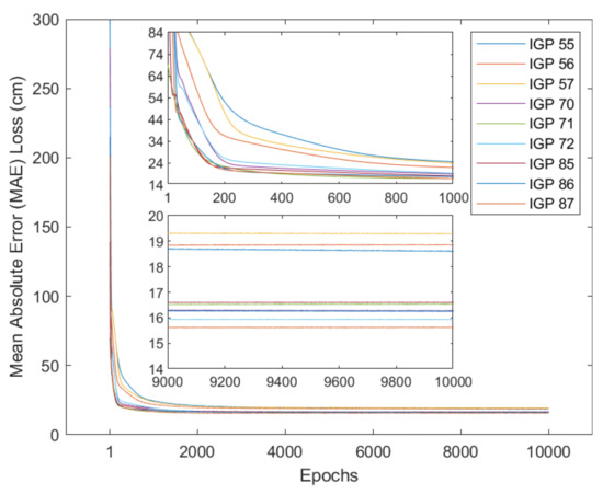
Figure 5. Validation MAE losses in centimeters as a function of training epochs. There are two partially enlarged figures that show the details of the first and last 1000 epochs.

It is noticed from Figure 5 that loss functions concerning epochs are not smooth, and light oscillations occur between epochs. After 10,000 epochs, the final validation losses (possibly not the best in history) are between 15 and 20 cm.

4.1. Under Normal Ionospheric Conditions

Test data under normal ionospheric conditions are selected from the year 2021, and contain a total of 3427 data points from January to May. Details are introduced in Section 2.1. Before presenting the derivation results, we firstly define the residual evaluating indicators MAE, RMSE, and R by giving the following equations:

$$MAE=mean\left(\left|{\mathit{V}}_{ntest}-{\mathit{Y}}_{ntest}\right|\right)$$

(41)

$$RMSE=\sqrt{mean\left({\left|{\mathit{V}}_{ntest}-{\mathit{Y}}_{ntest}\right|}^2\right)}$$

(42)

$$R=\frac{\Sigma (V_j-mean\left({\mathit{V}}_{ntest}\right))(Y_j-mean\left({\mathit{Y}}_{ntest}\right))}{\sqrt{\Sigma {(V_j-mean\left({\mathit{V}}_{ntest}\right))}^2\Sigma {(Y_j-mean\left({\mathit{Y}}_{ntest}\right))}^2}}$$

(43)

where $V_j$ represents the predicted GIVD for ANNs or fitted GIVD for other methods; $Y_j$ is the corresponding reference which is acquired from CODE GIM final products. Table 2 shows the resulting MAE and RMSE of the fitting residuals under normal ionospheric conditions by applying various methods.

Table 2. Fitting residuals evaluated by MAE in centimeters under normal conditions.

	G55	G56	G57	G70	G71	G72	G85	G86	G87
Planar MAE	22.06	22.19	22.67	19.06	18.58	19.28	19.18	17.72	17.27
Kriging MAE	23.05	23.63	23.30	17.53	18.72	19.04	17.37	17.14	17.07
ANN MAE	18.39	18.31	18.99	14.54	14.23	13.73	14.49	13.92	13.97
Planar RMSE	27.94	28.45	29.76	24.14	22.90	24.06	23.60	21.48	21.05
Kriging RMSE	29.97	30.92	30.97	21.90	23.22	23.37	20.95	20.74	20.53
ANN RMSE	23.89	24.15	25.53	18.59	17.91	17.24	18.55	17.64	17.71

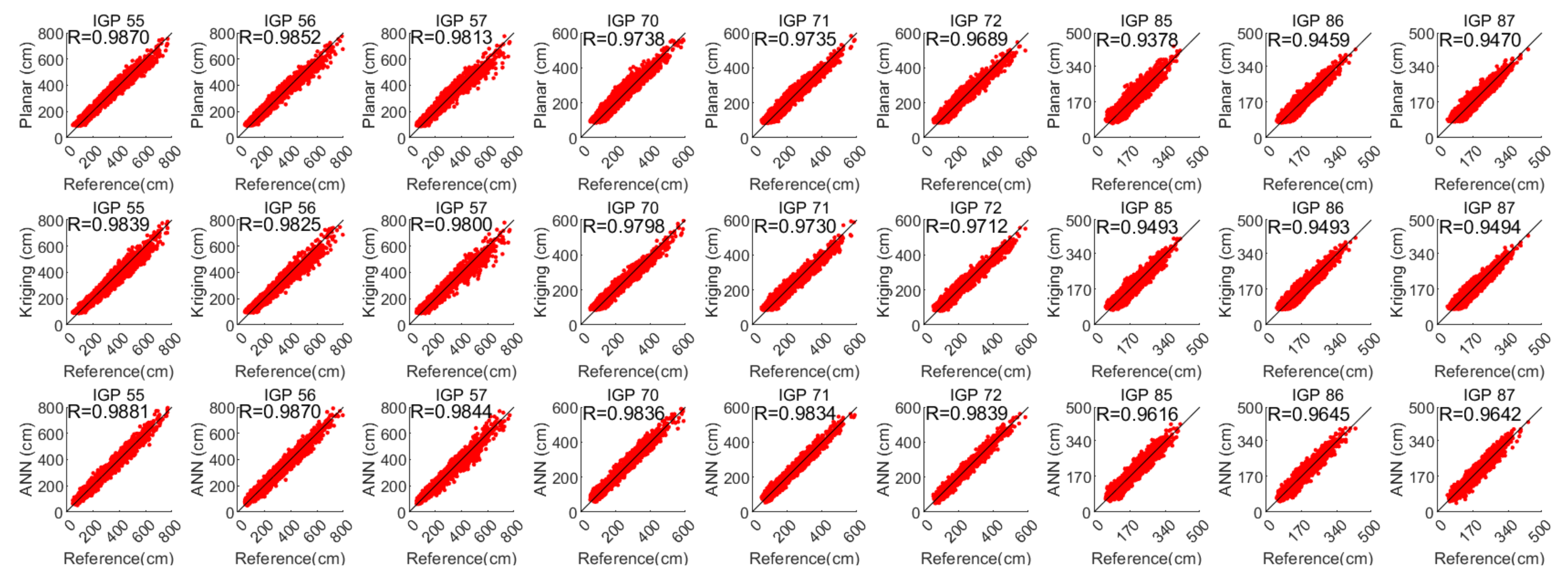
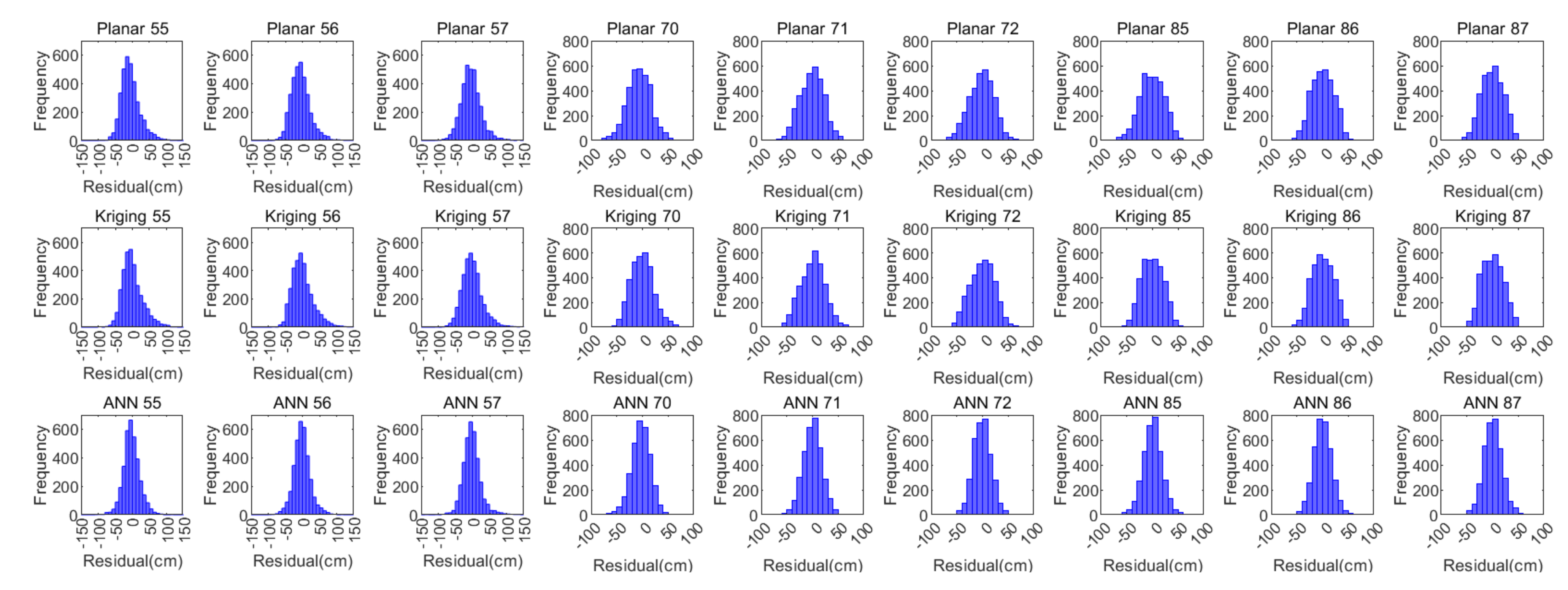
To intuitively reveal the fitting accuracy and residual distribution of each existing and proposed method, the following Figure 6 shows the predicted GIVDs by applying various methods as a function of their corresponding references. The residual (reference minus the predicted) distribution histograms are generated. The evaluating indicator R for each IGP and each method is also calculated and presented in Figure 7.

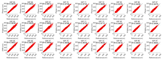
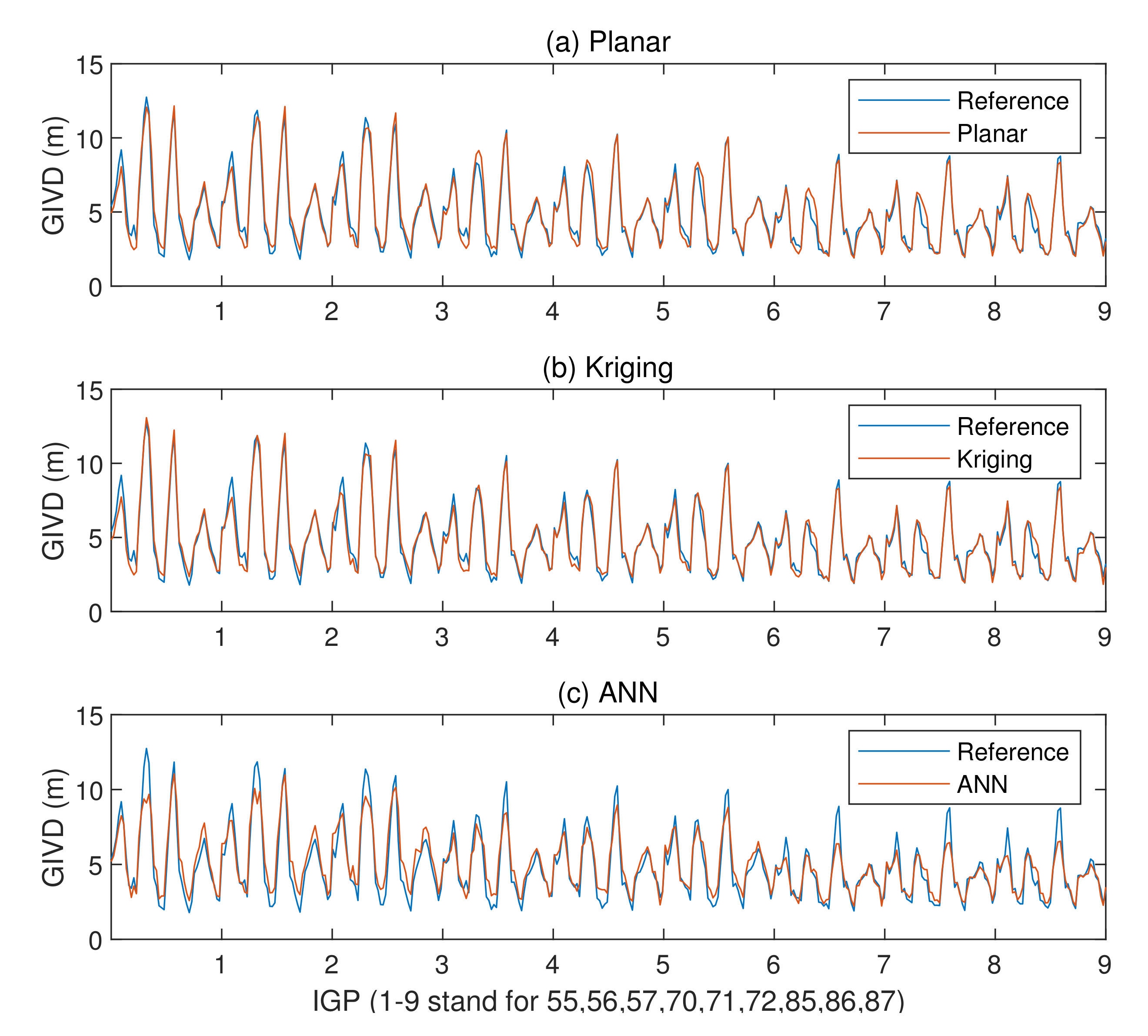
Figure 6. Predicted GIVD applying planar fit, Kriging, and ANN methods with respect to the references.

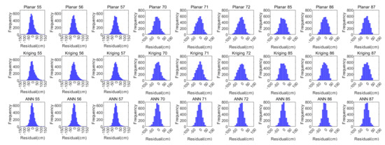
Figure 7. Residual histograms of the planar fit, Kriging, and ANN ionospheric methods.

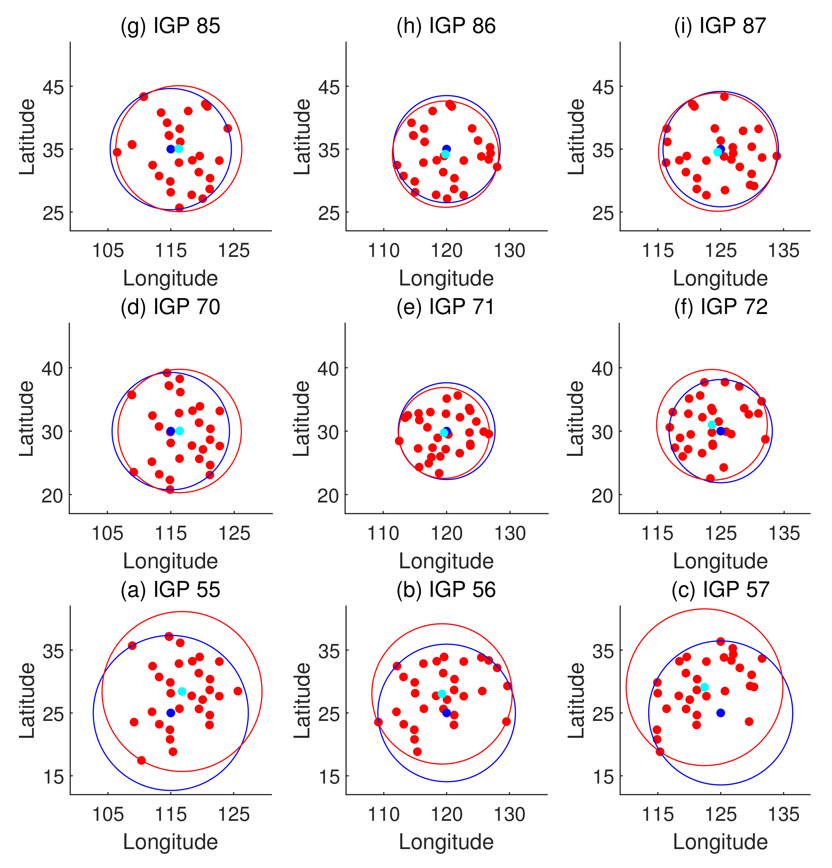
It is known that the fitting accuracy is affected by the accuracy of IPP vertical delay extraction. The Hatch filter-smoothed code measurements are adopted in this connection. Moreover, the distribution of IPPs relative to the IGP is also a dominant factor that affects the predicted accuracy. Once locations of the reference stations and constellations used are determined, the typical distributions of the IPPs are hardly changed. Figure 8 presents the typical distributions of IPPs around each IGP.

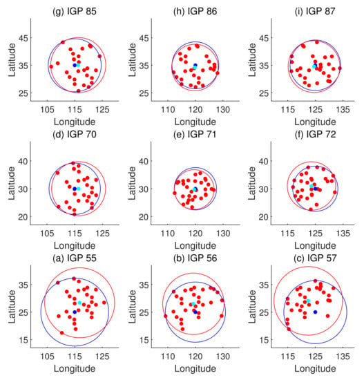
Figure 8. Typical distributions of IPPs around each IGP. IPPs are represented by red dots; cyan dots and corresponding red circles show the focuses of IPPs and range covering the farthest IPP; blue dots and corresponding circles are IGPs and range covering the farthest IPP, which also imply the fitting radius.

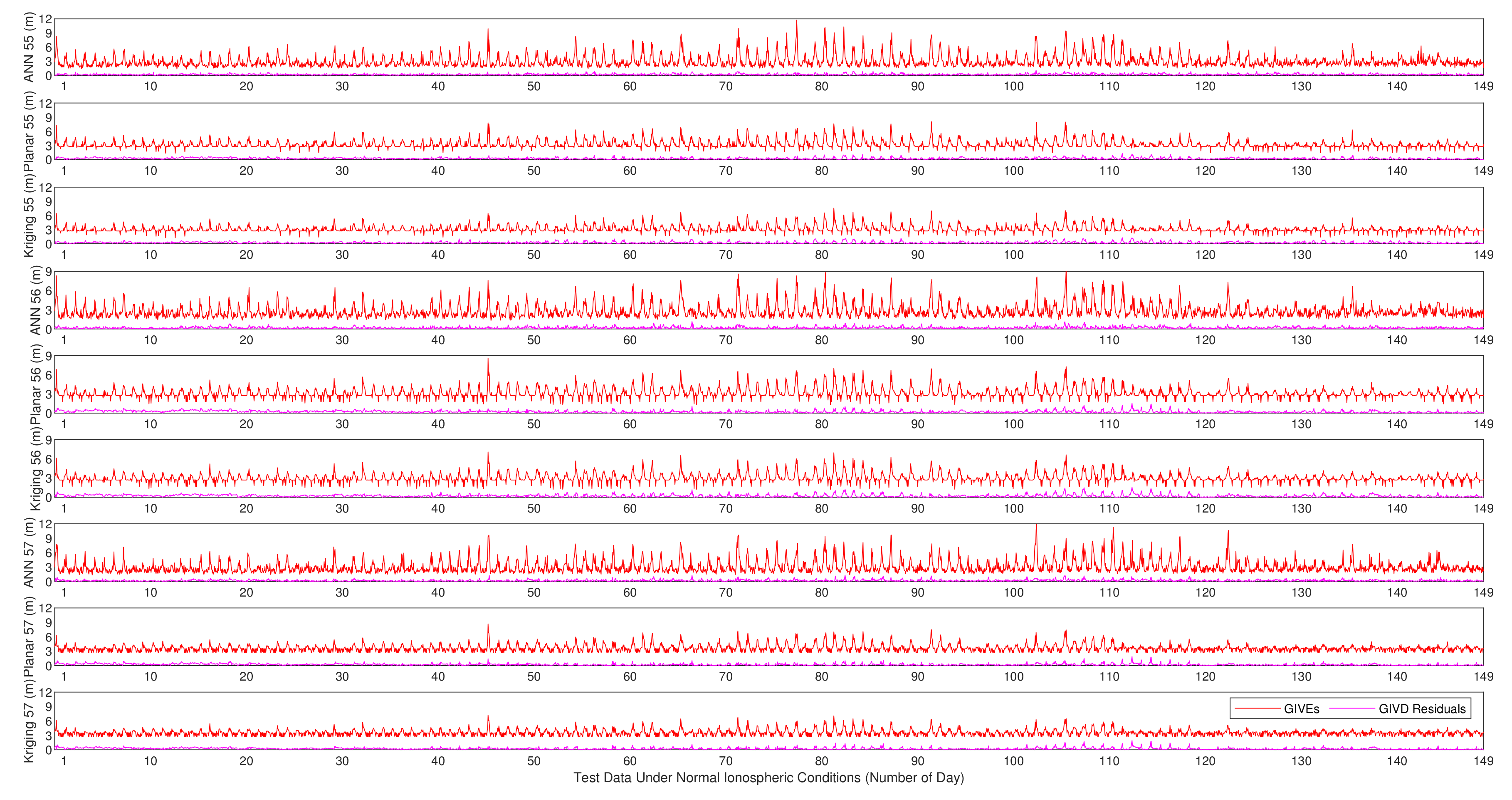
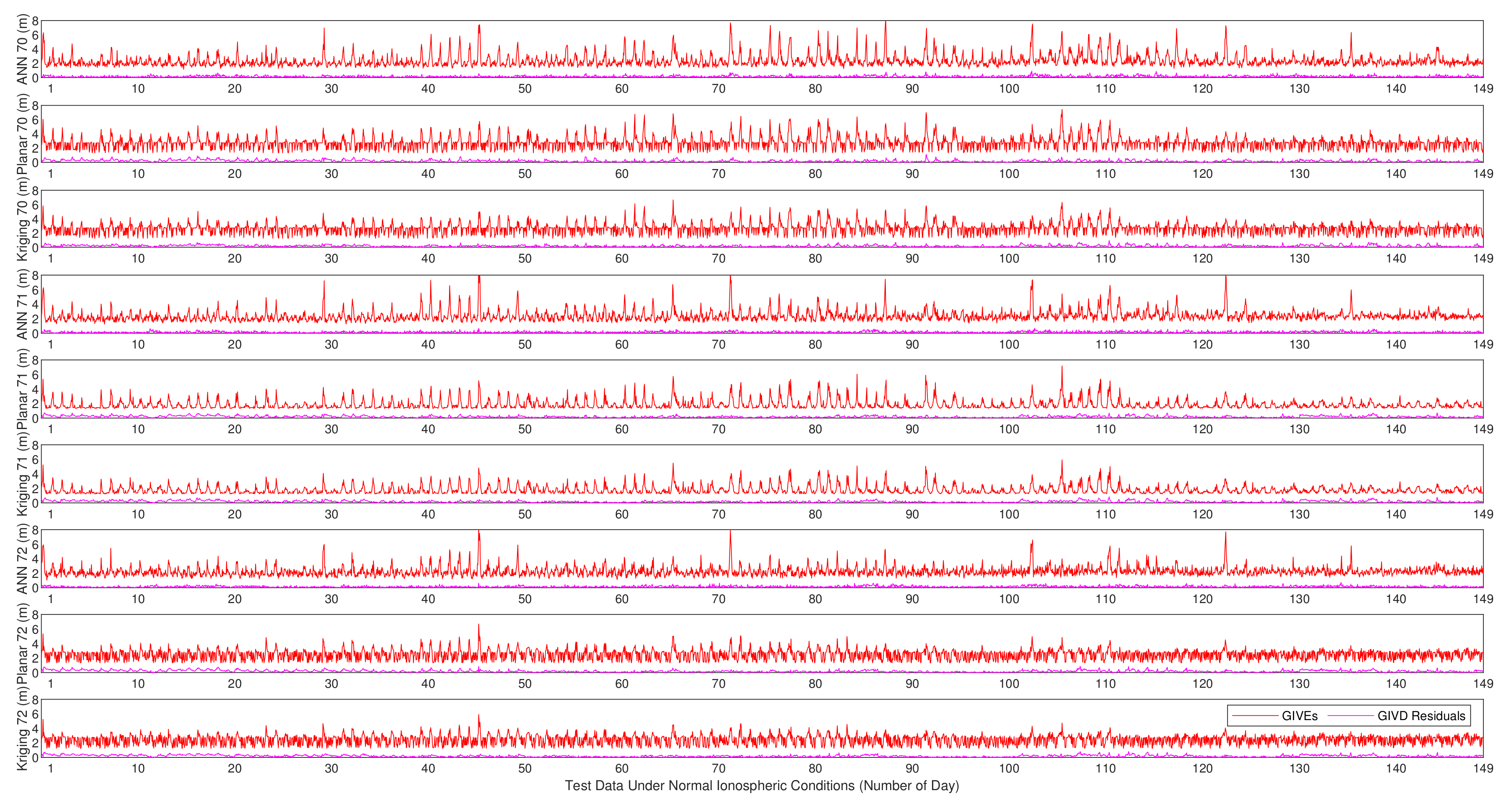
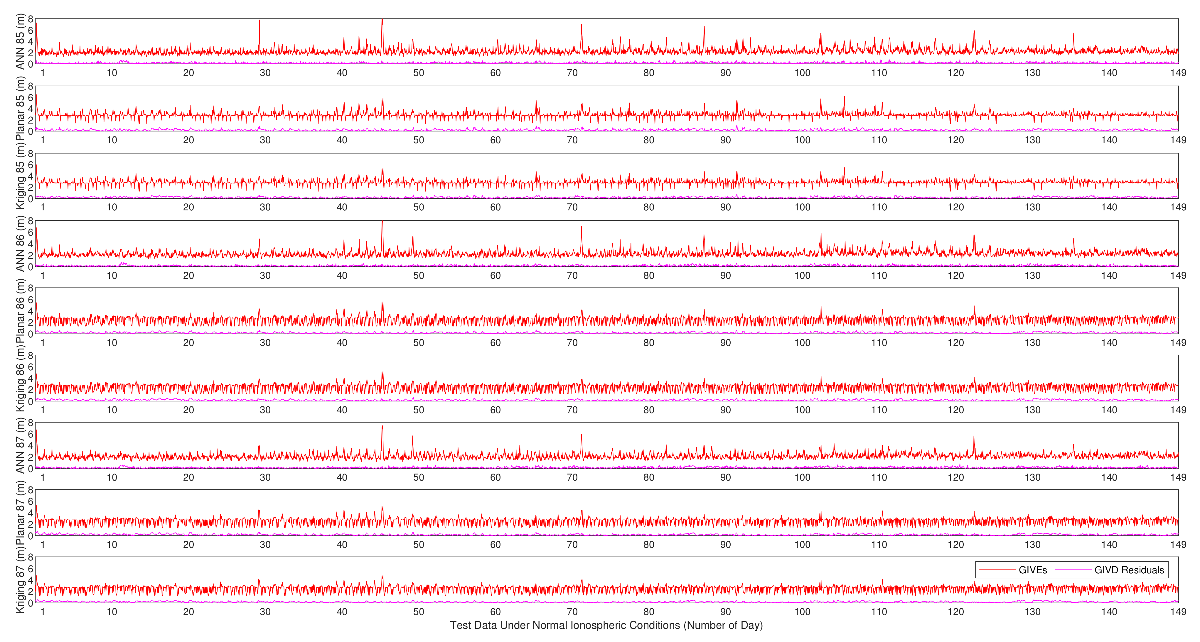
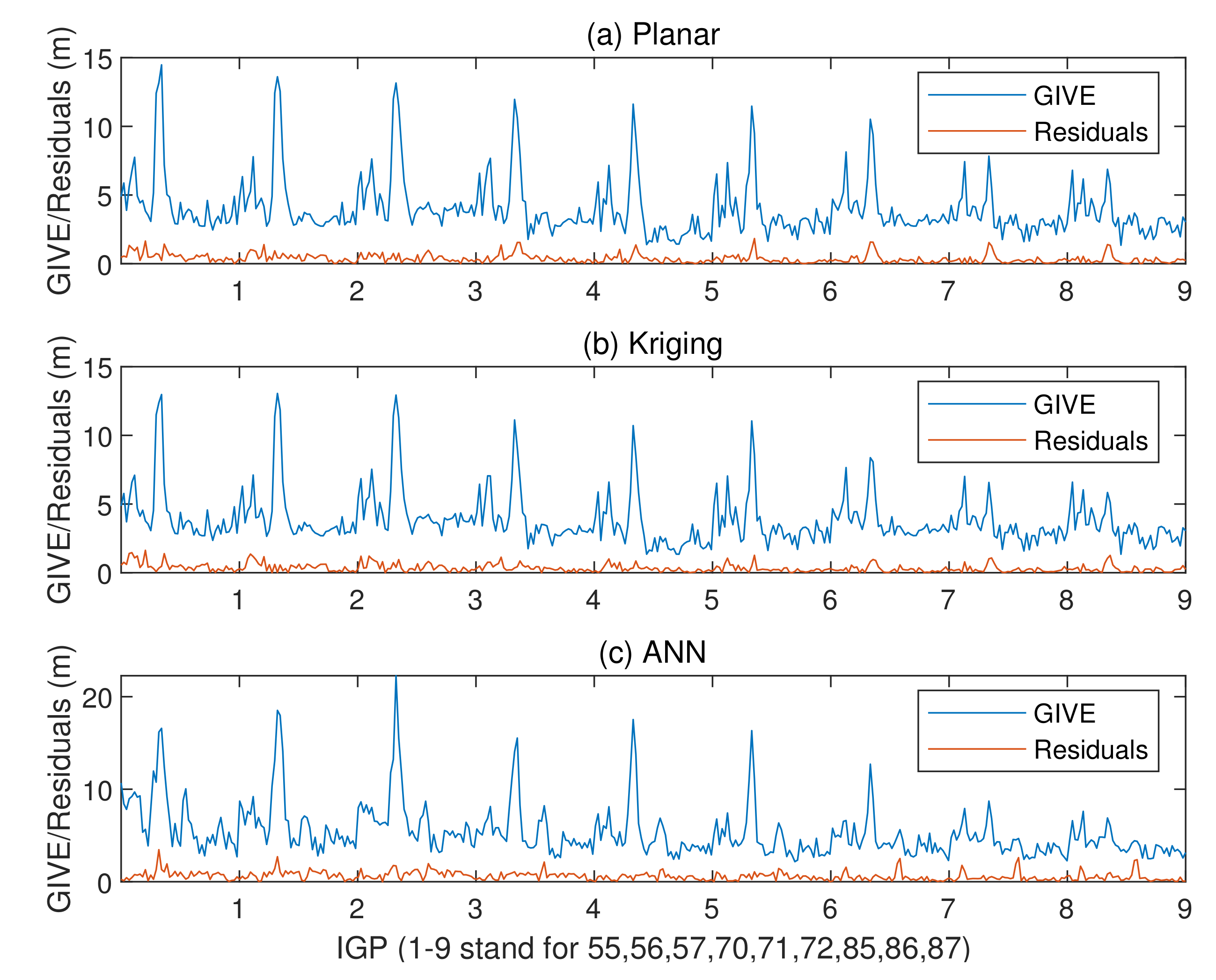
GIVE provides the confidence bounds for GIVD residuals and is an essential index of SBAS integrity. To a certain extent, the reliability of GIVE estimation is more significant than the accuracy of GIVD estimation in the SBAS. Figure 9, Figure 10 and Figure 11 present the absolute values of the GIVD residuals with corresponding GIVEs applying the planar fit, Kriging, and ANN methods for contrastive purposes. For each IGP, ANN data are firstly printed, then followed by the planar fit, and then by Kriging data. Table 3 records the average and maximum values of the bounding error ratios for different methods. The bounding error ratio is defined as the absolute residual divided by its GIVE [37].

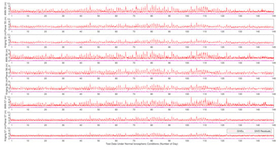
Figure 9. Vertical delay residuals and corresponding GIVEs applying various methods on IGP 55, IGP 56, and IGP 57 under normal ionospheric conditions.

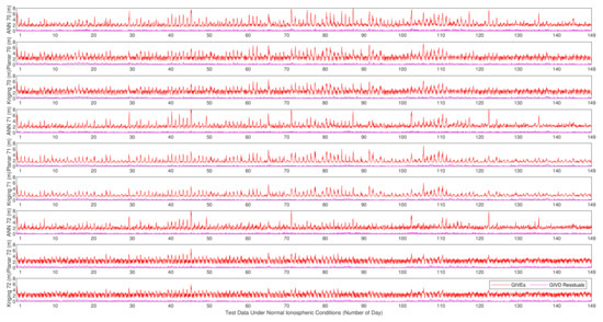
Figure 10. Vertical delay residuals and corresponding GIVEs applying various methods on IGP 70, IGP 71, and IGP 72 under normal ionospheric conditions.

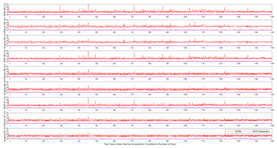
Figure 11. Vertical delay residuals and corresponding GIVEs applying various methods on IGP 85, IGP 86, and IGP 87 under normal ionospheric conditions.

Table 3. The average and maximum bounding error ratios in percentages of the planar fit, Kriging, and ANN methods under normal ionospheric conditions.

	G55	G56	G57	G70	G71	G72	G85	G86	G87
Planar AVG	6.89	7.17	6.21	7.22	10.48	8.22	6.61	7.65	7.05
Kriging AVG	7.35	7.72	6.46	7.03	11.01	8.39	6.16	7.54	7.16
ANN AVG	6.50	6.86	6.64	6.52	6.23	6.48	6.71	6.33	6.68
Planar MAX	39.78	52.38	52.60	34.00	44.07	45.86	24.82	41.27	35.47
Kriging MAX	45.55	53.67	53.41	41.83	49.14	52.37	28.85	37.46	37.94
ANN MAX	38.59	60.89	55.82	37.01	32.68	33.04	36.91	37.85	38.21

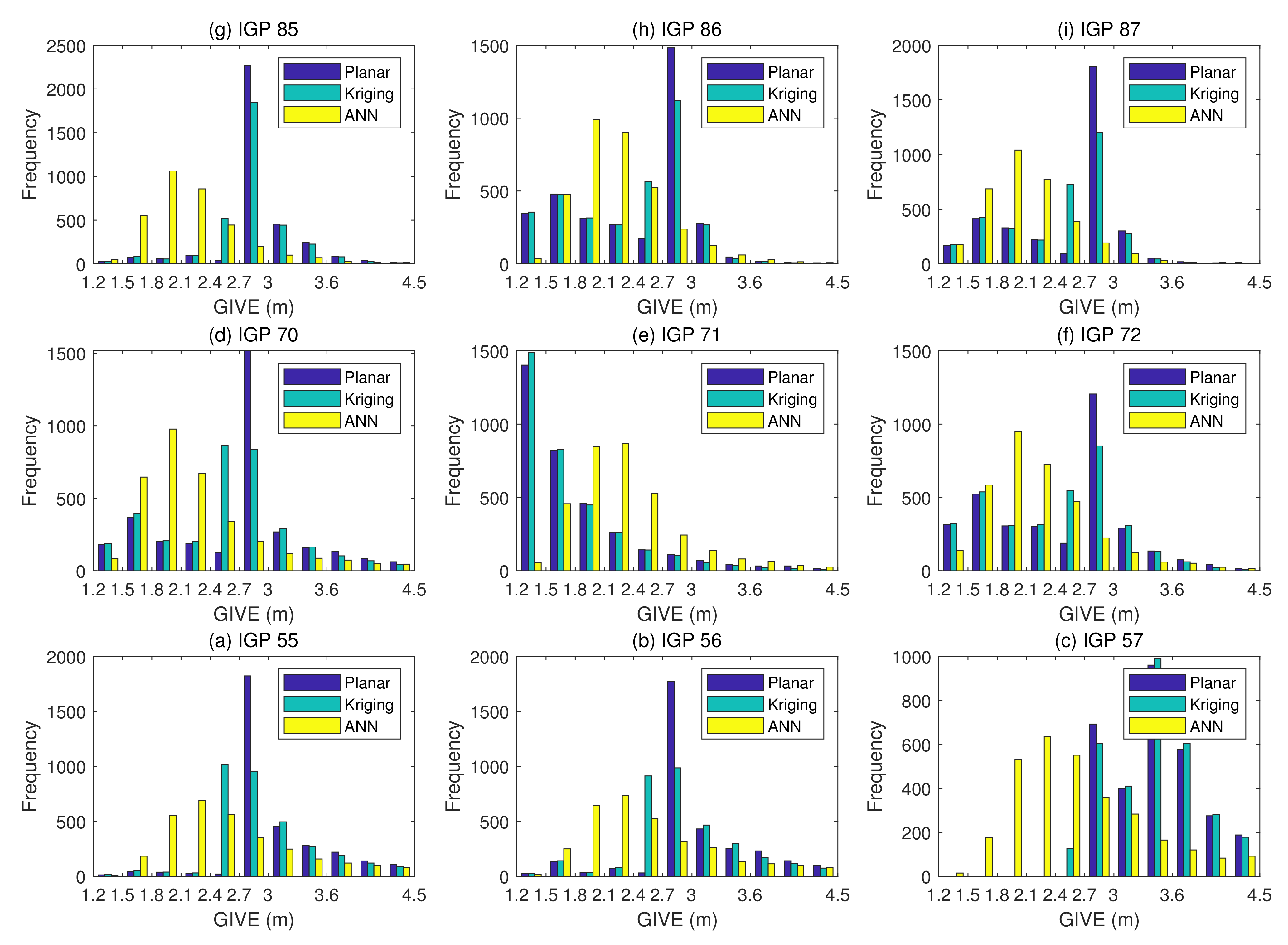
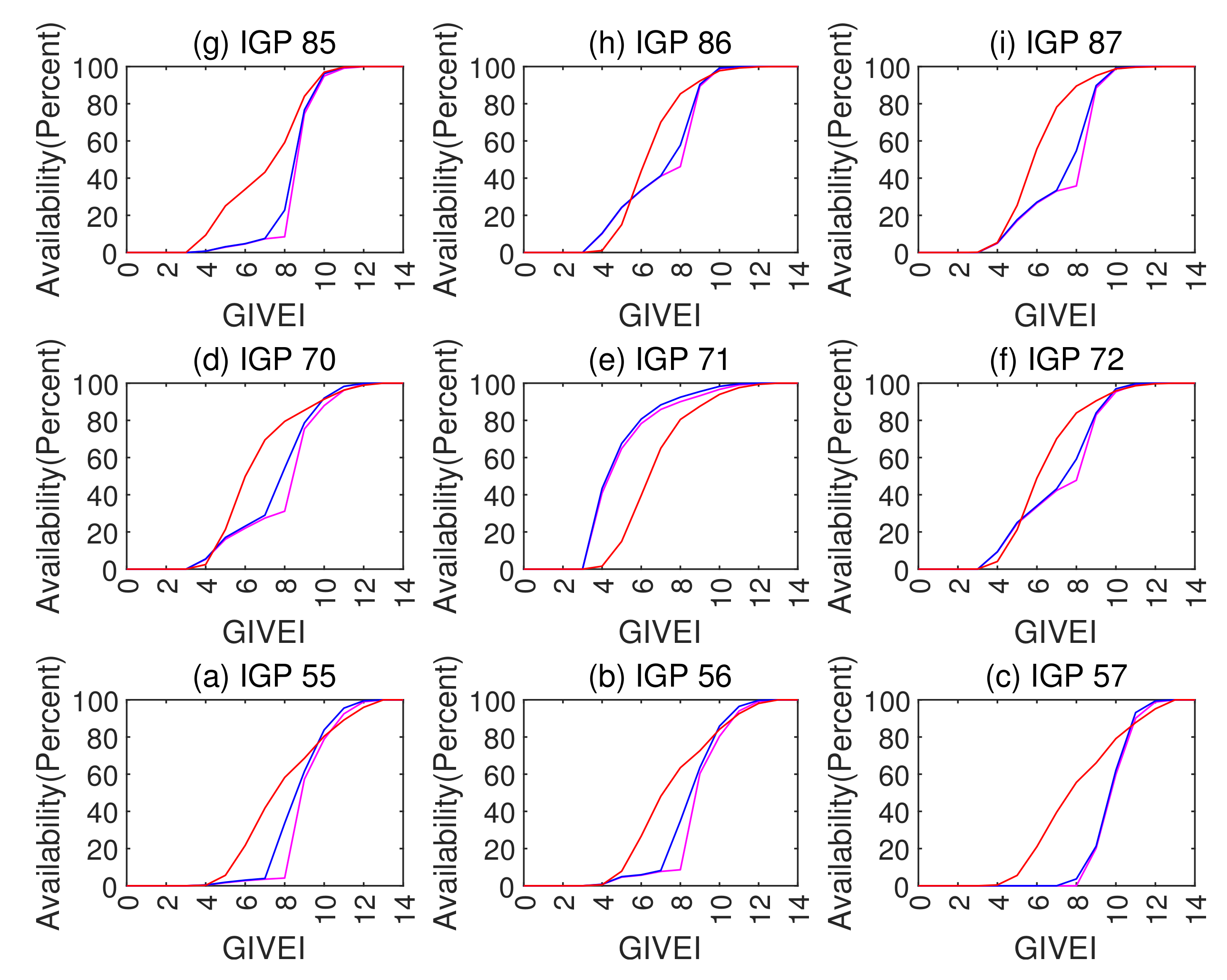
The Grid Ionospheric Vertical Error Indicator (GIVEI) is the discrete form of GIVE representation for message convenience [11]. Figure 12 presents the GIVE histograms of the planar fit, Kriging, and ANN GIVE methods. The GIVE partitions on the abscissa axis are divided according to GIVEI 3 to 11. Figure 13 shows the GIVEI availability distributions under normal ionospheric conditions.

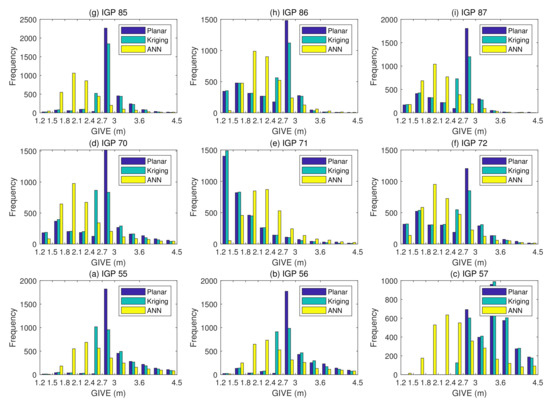
Figure 12. GIVE histograms of the planar fit, Kriging, and ANN methods under normal ionospheric conditions.

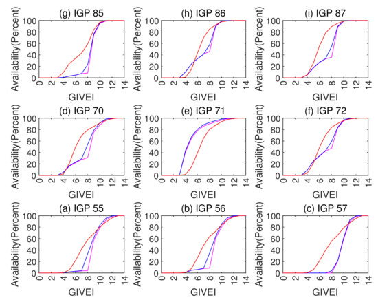
Figure 13. GIVEI availability in percentages of various methods under normal conditions. The planar fit method is shown as purple lines; Kriging method is represented by blue; ANN method is shown in red.

GIVE values below 2.7 m and 6.0 m in percentages are listed in the following Table 4. The ANN method has at least 25 percentage points more on most IGPs for 2.7 m GIVE availability.

Table 4. GIVE 2.7 m and 6.0 m availability in percentages of the planar fit, Kriging, and ANN methods under normal ionospheric conditions.

	G55	G56	G57	G70	G71	G72	G85	G86	G87
Planar 2.7 m	4.14	8.60	0	31.14	90.05	47.77	8.46	46.19	35.80
Kriging 2.7 m	33.64	34.84	3.68	54.30	92.47	59.18	22.79	57.69	54.71
ANN 2.7 m	58.24	63.50	55.62	79.46	80.84	83.98	86.37	85.32	89.52
Planar 6.0 m	98.95	99.18	98.80	99.47	99.94	99.97	99.94	100	100
Kriging 6.0 m	99.47	99.74	99.42	99.91	100	100	100	100	100
ANN 6.0 m	95.97	98.07	95.16	98.95	99.39	99.71	99.77	99.85	99.88

4.2. Under Disturbed Ionospheric Conditions

Test data under disturbed ionospheric conditions are selected from 2012 and 2013, containing a total of 44 data points. Data for disturbed conditions are sparse for several reasons: total ionospheric disturbed days are rare in the past decade; days before 2016 are selected due to not overlapping in time with training and validation data; all observation files of seven stations need to be intact on selected days.

Due to the small amount of test data under disturbed conditions, reference prediction figures and residual histograms are not convincing. Therefore, we just put forward the figure of predicted GIVDs by various methods as well as their references, data point by data point. Residual indicators MAE and RMSE are presented in tables. Figure 14 shows the predicted GIVDs by multiple methods and the CODE GIM references of each data point. Table 5 records the resulting MAE and RMSE of the fitting residuals under disturbed conditions by applying various methods.

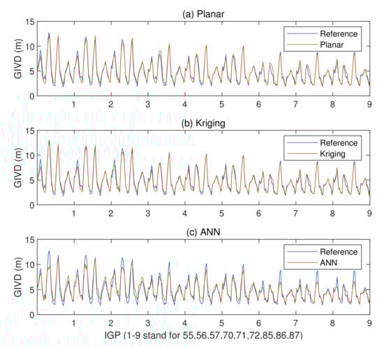
Figure 14. Derived GIVDs and CODE GIM references in meters under disturbed conditions.

Table 5. Fitting residuals evaluated by MAE in centimeters under disturbed conditions.

	G55	G56	G57	G70	G71	G72	G85	G86	G87
Planar MAE	55.65	45.31	40.65	42.46	30.46	31.34	32.05	27.05	27.21
Kriging MAE	51.27	41.84	41.63	34.36	27.23	27.78	24.66	24.29	26.66
ANN MAE	76.38	77.50	87.91	60.05	53.21	54.92	42.01	41.30	46.34
Planar RMSE	66.19	54.15	47.50	55.25	41.65	44.17	47.26	40.41	39.94
Kriging RMSE	64.25	53.30	52.14	41.44	35.40	37.32	33.53	34.15	37.18
ANN RMSE	99.08	92.08	100.2	73.28	63.05	63.33	64.13	62.40	68.82

Figure 15 presents the absolute vertical delay residuals and corresponding GIVEs derived by three methods under disturbed ionospheric conditions. Meanwhile, the averaged and maximum bounding error ratios of GIVE under abnormal conditions are shown in Table 6.

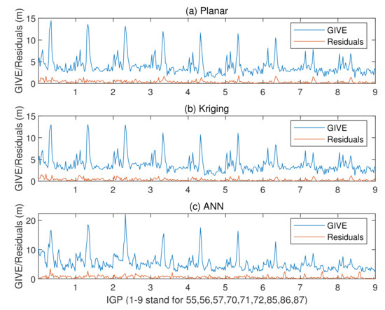
Figure 15. Vertical delay residuals and corresponding GIVEs by applying various methods under disturbed ionospheric conditions.

Table 6. The average and maximum bounding error ratios in percentages of the planar fit, Kriging, and ANN methods under disturbed ionospheric conditions.

	G55	G56	G57	G70	G71	G72	G85	G86	G87
Planar AVG	13.03	11.20	8.96	10.51	10.06	8.26	7.28	7.84	7.68
Kriging AVG	12.41	10.99	8.93	9.23	9.73	7.84	6.11	7.32	7.83
ANN AVG	12.28	13.64	14.92	13.64	11.12	13.30	10.17	11.37	10.75
Planar MAX	42.93	33.27	21.85	32.93	31.74	19.48	18.35	27.68	22.90
Kriging MAX	43.18	29.54	23.11	28.53	31.29	19.34	16.84	25.52	24.63
ANN MAX	36.49	41.99	43.45	32.88	34.71	35.19	44.55	55.67	54.50

4.3. Case of Insufficient IPPs

When the number of IPPs around an IGP for GIVD or GIVE derivation is insufficient, GIVDs and GIVEs of IGPs could be estimated if the number of IPPs is larger than $N_{min}=10$ by applying the planar fit and Kriging methods [16,20].

In this part, the resolvent of GIVDs and GIVEs by applying the ANN method for insufficient IPPs is given. IGPs 54 (25°N, 110°E), 68 (30°N, 105°E), and 83 (35°N, 105°E) that are distributed on the edge of the selected station network region are tested. Based on historical data, the minimum number of available IPPs around IGP 54 is 25, by applying the search algorithm proposed by Sparks [20]. The minimum numbers of available IPPs around IGP 68 and IGP 83 in history are 20 and 15, respectively.

Since the ANN has a fixed structure for a certain IGP, the input number of the network is also invariant. Therefore, we trim the network inputs for IGPs with insufficient IPPs. Specifically, this is carried out by trimming the dimensions of the input vectors ${\mathsf{\Phi }}_j$, ${\mathsf{\Lambda }}_j$, and ${\mathit{I}}_j$ to the minimum available IPP numbers, and adjusting the number of hidden layer neurons accordingly. As a result, the structures of ANNs for IGP 54, IGP 68, and IGP 83 are 78-26-1, 63-21-1, and 48-16-1.

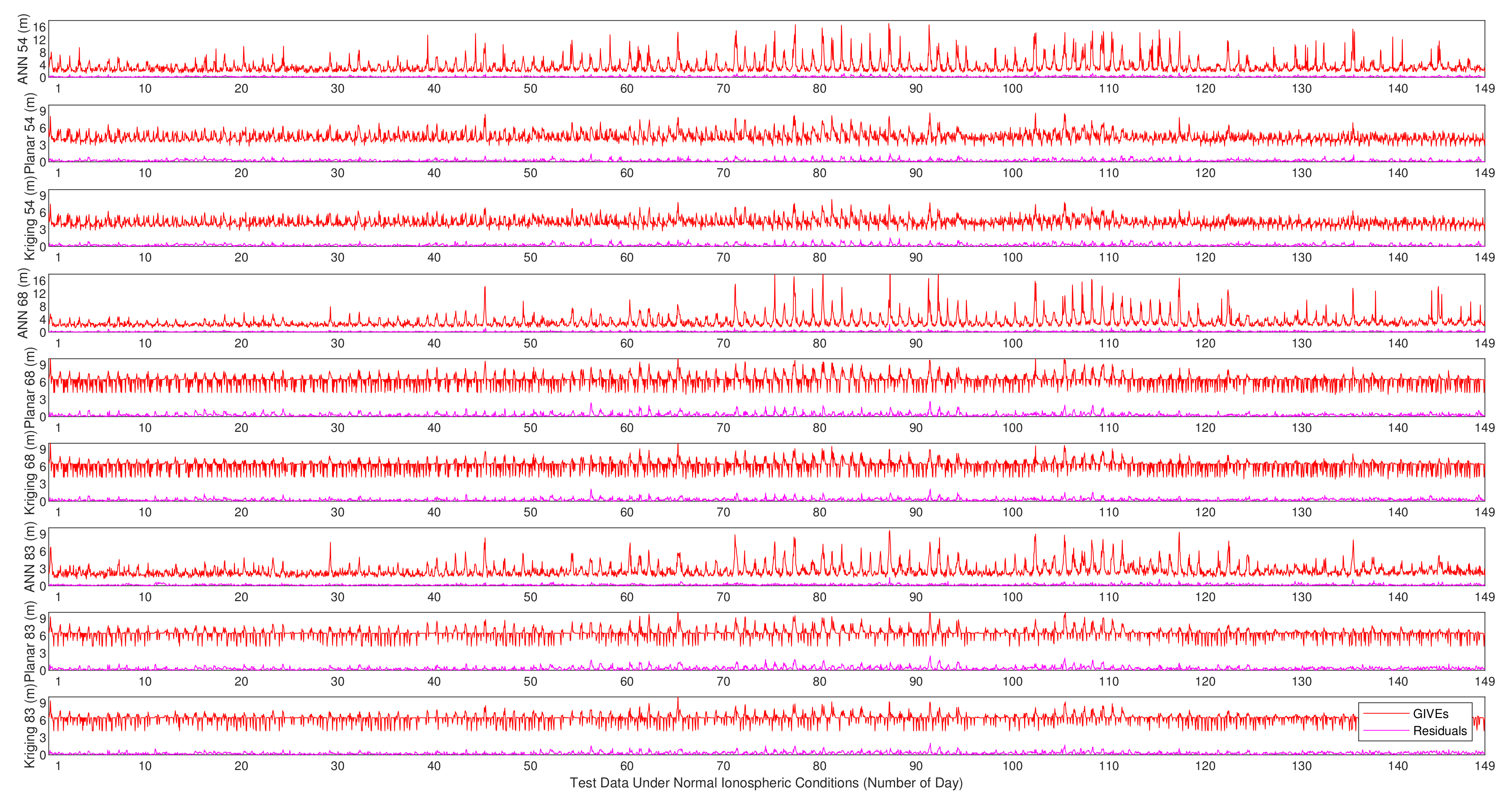
The experimental results on IGP 54, IGP 68, and IGP 83 by applying the planar fit, Kriging, and ANN methods are given below. When IPP numbers are larger than the minimum in history, the planar fit and Kriging methods adopt all the eligible IPPs. However, the ANN only uses the nearest minimum number of IPPs and abandons the others. Figure 16 and Figure 17 show the absolute values of the vertical delay residuals and corresponding GIVEs under normal and disturbed conditions, respectively. Table 7 presents the MAE and RMSE of the fitting residuals under different ionospheric conditions, and Table 8 records the average and maximum bounding error ratios of GIVEs.

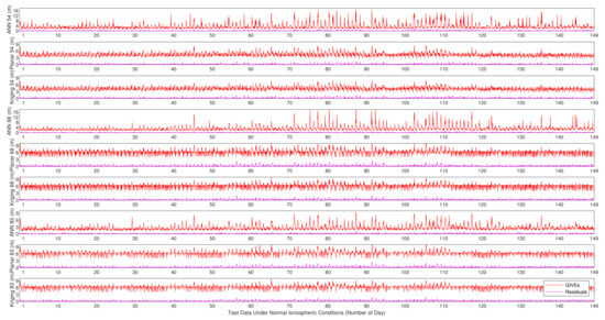
Figure 16. Vertical delay residuals and corresponding GIVEs by applying various methods on IGP 54, IGP 68, and IGP 83 under normal ionospheric conditions.

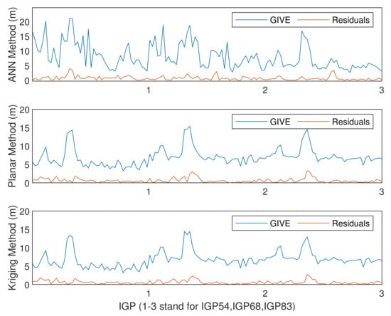
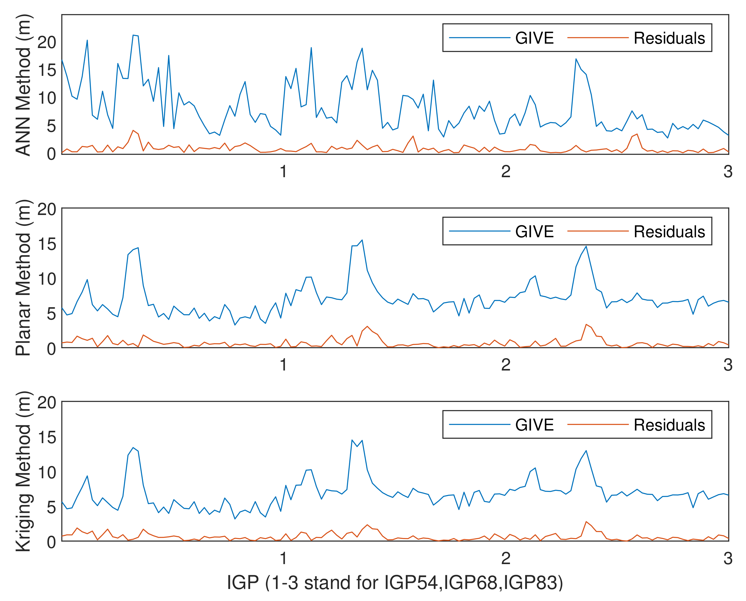
Figure 17. Vertical delay residuals and corresponding GIVEs by applying various methods under disturbed ionospheric conditions.

Table 7. Fitting residuals evaluated by MAE and RMSE in centimeters under different ionospheric conditions, NC for normal conditions, DC for disturbed conditions.

	G54 NC	G68 NC	G83 NC	G54 DC	G68 DC	G83 DC
Planar MAE	22.97	30.66	32.03	64.28	67.79	63.21
Kriging MAE	23.76	25.80	28.32	61.64	64.10	56.20
ANN MAE	19.55	16.93	15.49	91.78	71.08	52.98
Planar RMSE	30.45	42.91	43.10	78.12	97.34	92.52
Kriging RMSE	31.82	34.68	36.58	76.50	84.35	77.97
ANN RMSE	26.59	23.51	20.21	121.9	94.70	85.30

Table 8. The average and maximum bounding error ratios in percentages of the planar fit, Kriging, and ANN methods under different ionospheric conditions, NC for normal conditions, DC for disturbed conditions.

	G54 NC	G68 NC	G83 NC	G54 DC	G68 DC	G83 DC
Planar AVG	5.16	4.75	4.90	11.44	8.27	7.68
Kriging AVG	5.47	4.14	4.45	11.29	8.10	7.19
ANN AVG	6.23	5.62	6.23	10.86	8.43	8.71
Planar MAX	25.82	28.52	25.96	31.27	27.61	25.25
Kriging MAX	30.71	25.99	23.32	31.05	22.90	21.48
ANN MAX	46.34	32.35	34.55	29.34	31.26	55.39

5. Discussion

Scrutinizing Table 2 and Figure 5, the ANN prediction residuals in the MAE of test data under normal conditions are similar to the validation MAE losses and even better. This phenomenon shows that the ANN captures the fitting regulations by learning numerous data and does not overfit them. The planar fit and Kriging methods perform similarly, which verifies the statement made by Sparks in [20]. The MAE and RMSE residual reductions in the ANN method are approximately 15% relative to planar fit and Kriging under normal ionospheric conditions among tested IGPs.

From Figure 8, which describes the distribution of IPPs, it is noticed that low latitude IGPs 55, 56, and 57 have dispersed surrounding IPPs and deviated IPP focuses. Accordingly, the residual distributions of the planar fit and Kriging methods emerge in a non-Gaussian form in the histograms shown in Figure 7. In contrast, the residual distributions for the other six IGPs at higher latitudes with concentrative and centric surrounding IPPs are more likely to meet the Gaussian distribution. However, the residuals of GIVDs predicted by the ANN method almost perfectly meet the Gaussian distribution regardless of the IPP scattering or eccentricity. Therefore, the ANN method maintains the fitting performance of IGPs at the edges of the SBAS service area. Furthermore, Figure 6 shows that the ANN method achieves the most centralized reference prediction plots and maximal R values, which symbolizes the best correlations between predicted and reference vertical delays.

It is found from Figure 9, Figure 10 and Figure 11 that, in general, GIVE fluctuates daily, and most residuals also follow the trend. GIVD residuals and GIVE crests often emerge when the solar altitude angle reaches maximum. Since low latitude IGPs 55, 56, and 57 have more active ionospheric states, the top values of GIVEs during the tested period (149 days) are between 9 m and 12 m. In contrast, the maximum GIVEs of other IGPs at higher latitudes are less than 8 m.

From Figure 9, Figure 10 and Figure 11, it is also noticed that although the ANN method is completely different from the planar fit and Kriging methods in the principle of GIVE derivation, they give similar GIVE estimations at corresponding time points. The consistency of GIVE results makes the methods mutually confirm their rationality. It is also noticed that ANN GIVEs for active ionospheric status (GIVE peaks) are more conservative than other methods. On the contrary, the flat parts of ANN GIVEs are more radical than that of the planar fit and Kriging methods, i.e., the ANN GIVE method provides lower confidence bounds on static ionospheric status. Nevertheless, the average bounding error ratio presented in Table 3 proves that the ANN GIVE method is the most conservative under normal ionospheric conditions among the three. The maximum ratios in Table 3 imply that no residual exceeds the GIVE bounds.

Combining Figure 12 and Figure 13, it could be found that on most IGPs, the ANN GIVE method provides smaller error bounds than other methods. In addition, IGP 71 has perfect IPP distributions in most cases. Therefore, the GIVEs derived by the planar fit and Kriging methods are better than the ANN method.

In the GIVEI availability in Figure 13, the ANN method ascends more rapidly than the planar fit and Kriging methods at the early stage (small GIVEI), while at the later stage (large GIVEI), planar and Kriging methods rise more rapidly and reach 100% earlier. This property accords with Figure 9, Figure 10 and Figure 11 that show that the ANN GIVE method provides radical bounds for small errors and conservative bounds for large errors.

Under disturbed ionospheric conditions, the prediction accuracy of the ANN method falls behind the other two methods which is corroborated by Figure 14 and Table 5. The Kriging method attains the best accuracy. The fitting residuals of Kriging are 10% lower than that of the planar fit method on most IGPs. It is found from Figure 14 that the ANN-predicted GIVDs are basically consistent with the references. Nevertheless, the prediction errors at several ionospheric delay peaks approach 3 m, which tremendously drag down the total accuracy. Under disturbed conditions, ANNs are unable to make good predictions when large distinctions exist between testing data and training data. The losses of minimal samples are sacrificed so that the network maintains a minimum total loss during the training process.

In Figure 15, the varying GIVE trends of different methods are still consistent, which is reflected by the locations of peaks and troughs. Consequently, the ANN GIVE method is effective under extremely active ionospheric conditions. However, under disturbed conditions, the conservative GIVE of the ANN method is obviously manifested, which will restrict the system’s availability. The 2.7 m GIVE availabilities averaged from all IGPs of the planar fit, Kriging, and ANN methods are 14.90%, 18.94%, and 5.05%, and the 6.0 m availabilities are 88.64%, 90.15%, and 72.22%, respectively, under disturbed conditions.

In Table 6, the average bounding error ratios are increased compared to normal conditions. The rising ratios in planar fit and Kriging methods are conventional due to the design of the GIVE algorithm. However, in the ANN GIVE method, the ascending average bounding error ratios are deteriorated by anomalously enlarged residuals. Although the maximum bounding error ratios of the ANN method are still much less than 100%, there exist risks in the ANN GIVE method when lacking training data. In addition, it is noted that in order to deal with the influence of ionospheric random disturbance in the SBAS, some schemes have been proposed to mitigate or even overcome, as much as possible, the adverse effects due to mathematical methods (modeling, interpolation, etc.) [38,39].

Based on the results provided by Figure 16 and Figure 17 and Table 7 and Table 8, in the case of insufficient IPPs, the fitting accuracy of planar fit and Kriging methods obviously declines, which can be evaluated by MAE and RMSE. However, the accuracy of the ANN method declines slightly due to the assistance of time, solar, and geomagnetic information. In addition, GIVEs derived by multiple methods are even more conservative, and the 2.7 m and 6.0 m GIVE availabilities of the ANN method are better than the other two methods on most IGPs.

6. Conclusions

Ionospheric delay is a critical error source in Global Navigation Satellite Systems (GNSSs) and a principal aspect of the SBAS corrections. Ionospheric vertical delays on IGPs that broadcast to users are derived from the IPPs observed by SBAS reference stations. Consequently, the ionospheric correction method is extremely important for the accuracy, integrity, and availability of navigation systems. However, traditional ionospheric methods just take the spatial specificities into consideration, ignoring the temporal correlations. In order to improve the system’s accuracy and integrity, the ANN-based ionospheric method is proposed in this article. Both temporal features and abundant historical data are applied for network training. Furthermore, based on the distribution of the residual random variable, the ANN-based GIVE algorithm is also derived.

In this study, when the number of IPPs around an IGP is above 30, the ANN model has a 93–31–1 three-layer structure. The 93 input features are 2-dimensional time indication, 1-dimensional geomagnetic and solar activity index derived by applying the Principal Component Analysis (PCA) technique, and 30 by 3-dimensional IPP relative latitudes, relative longitudes, and vertical delays. Other characters of the networks include selecting the sigmoid function as the hidden layer activation function and applying the Adam optimizer as the gradient updating algorithm. For each IGP, the network is trained and validated by a total of 30,130 data points selected from 2016 to 2020. Nine IGPs over the East China region are tested under normal and disturbed ionospheric conditions. GIVDs and accompanying GIVEs are calculated, for comparison with the planar fit and Kriging methods.

The derivation accuracy under normal ionospheric conditions is tested on 3427 data points collected from January to May 2021, while the accuracy under disturbed conditions is tested on 44 data points selected from 2012 and 2013. Results show that the MAE and RMSE of the ANN method are approximately 15% less than the planar fit and Kriging methods. Under disturbed conditions, on the contrary, the ANN is incompetent and shows the worst prediction accuracy, because of the minimal samples in the training set. Kriging retains a good performance and the fitting residuals of Kriging are 10% lower than that of planar fit on most IGPs.

On most tested IGPs under normal conditions, the ANN method provides smaller GIVEs and the residuals meet Gaussian distribution better than the other two methods. Specifically, the percentage of GIVE values below 2.7 m by applying the ANN method has at least 25 points more than Kriging. Under disturbed ionospheric conditions, the ANN GIVE method is still effective and conservative. However, the GIVE availability decline is evident in all GIVE Indicator (GIVEI) levels. Even though the residuals are far from bounding limits, the ANN GIVE method involves risks because of the minimal samples of the training dataset.

When the number of IPPs around an IGP is insufficient, the structures of ANNs are changed for three tested IGPs based on their available IPP number. The accuracy of the ANN method declines slightly, and 2.7 m and 6.0 m GIVE availabilities of the ANN method are better than the other two methods on most IGPs. Nevertheless, the regional and boundary performance of the ANN method in China could not be generalized until a large amount of the service area and all the edge IGPs are tested.

As a result, an ionospheric delay threshold should be set which indicates that the ANN model is not reliable. Training strategy optimization for the ANN method aiming at disturbed ionospheric conditions will be the research direction. GIVD and GIVE on IGPs over China by way of the ANN method will be discussed in the future.

References

- ICAO. Annex 10—Aeronautical Telecommunications—Volume I—Radio Navigational Aids, 8th ed.; International Civil Aviation Organization: Montreal, QC, Canada, 2018. [Google Scholar]
- Segura, D.I.; Garcia, A.R.; Alonso, M.T.; Sanz, J.; Juan, J.M.; Casado, G.G.; Martinez, M.L. EGNOS 1046 Maritime Service Assessment. Sensors 2020, 20, 276. [Google Scholar] [CrossRef] [PubMed] [Green Version]
- RTCA. Minimum Operational Performance Standards for Global Positioning System/Wide Area Augmentation System Airborne Equipment, DO-229D; Radio Technical Commission for Aeronautics (RTCA): Washington, DC, USA, 2013. [Google Scholar]
- Zhao, L.Q.; Hu, X.G.; Tang, C.P.; Cao, Y.L.; Zhou, S.S.; Yang, Y.F.; Liu, L.; Guo, R. Generation of DFMC SBAS corrections for BDS-3 satellites and improved positioning performances. Adv. Space Res. 2020, 66, 702–714. [Google Scholar] [CrossRef]
- Choy, S.; Kuckartz, J.; Dempster, A.G.; Rizos, C.; Higgins, M. GNSS satellite-based augmentation systems for Australia. Gps Solut. 2017, 21, 835–848. [Google Scholar] [CrossRef]
- Ciecko, A.; Bakula, M.; Grunwald, G.; Cwiklak, J. Examination of Multi-Receiver GPS/EGNOS Positioning with Kalman Filtering and Validation Based on CORS Stations. Sensors 2020, 20, 2732. [Google Scholar] [CrossRef] [PubMed]
- Nie, Z.X.; Zhou, P.Y.; Liu, F.; Wang, Z.J.; Gao, Y. Evaluation of Orbit, Clock and Ionospheric Corrections from Five Currently Available SBAS L1 Services: Methodology and Analysis. Remote Sens. 2019, 11, 411. [Google Scholar] [CrossRef] [Green Version]
- Chen, J.P.; Wang, A.H.; Zhang, Y.Z.; Zhou, J.H.; Yu, C. BDS Satellite-Based Augmentation Service Correction Parameters and Performance Assessment. Remote Sens. 2020, 12, 766. [Google Scholar] [CrossRef] [Green Version]
- Kim, M.; Kim, J. SBAS-Aided GPS Positioning with an Extended Ionosphere Map at the Boundaries of WAAS Service Area. Remote Sens 2021, 13, 151. [Google Scholar] [CrossRef]
- Schluter, S.; Hoque, M.M. An SBAS Integrity Model to Overbound Residuals of Higher-Order Ionospheric Effects in the Ionosphere-Free Linear Combination. Remote Sens. 2020, 12, 2467. [Google Scholar] [CrossRef]
- China Satellite Navigation Office. Available online: http://www.beidou.gov.cn/xt/gfxz/202008/P020200803362065480963.pdf (accessed on 26 January 2022).
- Yoon, H.; Seok, H.; Lim, C.; Park, B. An Online SBAS Service to Improve Drone Navigation Performance in High-Elevation Masked Areas. Sensors 2020, 20, 3047. [Google Scholar] [CrossRef]
- Liu, A.; Wang, N.; Li, Z.; Zhou, K.; Yuan, H. Validation of CAS’s final global ionospheric maps during different geomagnetic activities from 2015 to 2017. Results Phys. 2018, 10, 481–486. [Google Scholar] [CrossRef]
- Marini-Pereira, L.; Pullen, S.P.; Moraes, A.D. Reexamining Low-Latitude Ionospheric Error Bounds: An SBAS Approach for Brazil. IEEE Trans. Aerosp. Electron. Syst. 2021, 57, 674–689. [Google Scholar] [CrossRef]
- Zhang, Y.; Xiao, Z.B.; Liu, Z.; Tang, X.M.; Ou, G. SBAS performance improvement with a new undersampled ionosphere threat model based on relative coverage metric. J. Atmos. Sol.-Terr. Phys. 2020, 198, 105178. [Google Scholar] [CrossRef]
- Sparks, L.; Blanch, J.; Pandya, N. Estimating ionospheric delay using kriging: 2. Impact on satellite-based augmentation system availability. Radio Sci. 2011, 46. [Google Scholar] [CrossRef]
- Enge, P.; Walter, T.; Pullen, S.; Kee, C.; Chao, Y.-C.; Tsai, Y.-J. Wide area augmentation of the global positioning system. Proc. IEEE 1996, 84, 1063–1088. [Google Scholar] [CrossRef]
- Takka, E.; Belhadj-Aissa, A.; Yan, J.; Jin, B.; Bouaraba, A. Ionosphere modeling in the context of Algerian Satellite-based Augmentation System. J. Atmos. Sol.-Terr. Phys. 2019, 193, 105092. [Google Scholar] [CrossRef]
- Sparks, L.; Komjathy, A.; Mannucci, A.J. Sudden ionospheric delay decorrelation and its impact on the Wide Area Augmentation System (WAAS). Radio Sci. 2004, 39, 1–8. [Google Scholar] [CrossRef] [Green Version]
- Sparks, L.; Blanch, J.; Pandya, N. Estimating ionospheric delay using kriging: 1. Methodology. Radio Sci. 2011, 46, 1–13. [Google Scholar] [CrossRef]
- Trilles, S.; de la Hautiere, G.; van den Bossche, M. Adaptative Ionospheric Electron Content Estimation Method. I Navig. Sat. Div. Int. 2012, 46, 2307–2315. [Google Scholar]
- Yuan, Y.B.; Ou, J.K. Differential Areas for Differential Stations (DADS): A New Method of Establishing Grid Ionospheric Model. Chin. Sci. Bull. 2002, 47, 1033–1036. [Google Scholar] [CrossRef]
- Yuan, Y.B.; Ou, J.K. A Generalized Trigonometric Series Function Model for Determining Ionospheric Delay. Prog. Nat. Sci. 2004, 14, 1010–1014. [Google Scholar] [CrossRef]
- Sabzehee, F.; Farzaneh, S.; Sharifi, M.A.; Akhoondzadeh, M. TEC Regional Modeling and Prediction Using ANN Method and Single Frequency Receivers over IRAN. Ann. Geophys. 2018, 61, 103. [Google Scholar] [CrossRef] [Green Version]
- Inyurt, S.; Sekertekin, A. Modeling and predicting seasonal ionospheric variations in Turkey using artificial neural network (ANN). Astrophys. Space Sci. 2019, 364, 62. [Google Scholar] [CrossRef]
- Tebabal, A.; Radicella, S.M.; Damtie, B.; Migoya-Orue, Y.; Nigussie, M.; Nava, B. Feed forward neural network based ionospheric model for the East African region. J. Atmos Sol.-Terr. Phys. 2019, 191, 105052. [Google Scholar] [CrossRef]
- Okoh, D.; Habarulema, J.B.; Rabiu, B.; Seemala, G.; Wisdom, J.B.; Olwendo, J.; Obrou, O.; Matamba, T.M. Storm-Time Modeling of the African Regional Ionospheric Total Electron Content Using Artificial Neural Networks. Space Weather 2020, 18, e2020SW002525. [Google Scholar] [CrossRef]
- Mallika, I.L.; Ratnam, D.V.; Ostuka, Y.; Sivavaraprasad, G.; Raman, S. Implementation of Hybrid Ionospheric TEC Forecasting Algorithm Using PCA-NN Method. IEEE J.-Stars 2019, 12, 371–381. [Google Scholar] [CrossRef]
- Zhang, Z.X.; Pan, S.G.; Gao, C.F.; Zhao, T.; Gao, W. Support Vector Machine for Regional Ionospheric Delay Modeling. Sensors 2019, 19, 2947. [Google Scholar] [CrossRef] [PubMed] [Green Version]
- Kim, M.; Kim, J. Extending the coverage area of regional ionosphere maps using a support vector machine algorithm. Ann. Geophys. 2019, 37, 77–87. [Google Scholar] [CrossRef] [Green Version]
- Wen, Z.C.; Li, S.H.; Li, L.H.; Wu, B.W.; Fu, J.Q. Ionospheric TEC prediction using Long Short-Term Memory deep learning network. Astrophys. Space Sci. 2021, 366, 3. [Google Scholar] [CrossRef]
- Perez, R.O. Using TensorFlow-based Neural Network to estimate GNSS single frequency ionospheric delay (IONONet). Adv. Space Res. 2019, 63, 1607–1618. [Google Scholar] [CrossRef]
- Wang, S.; Wang, D.; Guan, Y.X. An Improved Ionospheric Delay Correction Method for SBAS. Chin. J. Electron. 2021, 30, 384–389. [Google Scholar]
- Jin, B.; Chen, S.S.; Li, D.J.; Takka, E.; Li, Z.S.; Qu, P.C. Ionospheric correlation analysis and spatial threat model for SBAS in China region. Adv. Space Res. 2020, 66, 2873–2887. [Google Scholar] [CrossRef]
- Kingma, D.P.; Ba, J.J. Adam: A method for stochastic optimization. In Proceedings of the 3rd International Conference for Learning Representations (ICLR), San Diego, CA, USA, 7–9 May 2015; pp. 1–15. [Google Scholar]
- Rivals, I.; Personnaz, L. Construction of confidence intervals for neural networks based on least squares estimation. Neural Netw. 2000, 13, 463–484. [Google Scholar] [CrossRef]
- Abe, O.E.; Paparini, C.; Ngaya, R.H.; Radicella, S.M.; Nava, B.; Kashcheyev, A. Assessment study of ionosphere correction model using single- and multi-shell algorithms approach over sub-Saharan African region. Adv. Space Res. 2019, 63, 3177–3188. [Google Scholar] [CrossRef]
- Yuan, Y.; Ou, J. An improvement to ionospheric delay correction for single-frequency GPS users—The APR-I scheme. J. Geod. 2001, 75, 331–336. [Google Scholar] [CrossRef]
- Yuan, Y.; Ou, J. Auto-covariance estimation of variable samples (ACEVS) and its application for monitoring random ionospheric disturbances using GPS. J. Geod. 2001, 75, 438–447. [Google Scholar] [CrossRef]
Publisher’s Note: MDPI stays neutral with regard to jurisdictional claims in published maps and institutional affiliations. |
© 2022 by the authors. Licensee MDPI, Basel, Switzerland. This article is an open access article distributed under the terms and conditions of the Creative Commons Attribution (CC BY) license (https://creativecommons.org/licenses/by/4.0/).