Tropical Cyclone Intensity Estimation Using Himawari-8 Satellite Cloud Products and Deep Learning

Abstract

This study develops an objective deep-learning-based model for tropical cyclone (TC) intensity estimation. The model’s basic structure is a convolutional neural network (CNN), which is a widely used technology in computer vision tasks. In order to optimize the model’s structure and to improve the feature extraction ability, both residual learning and attention mechanisms are embedded into the model. Five cloud products, including cloud optical thickness, cloud top temperature, cloud top height, cloud effective radius, and cloud type, which are level-2 products from the geostationary satellite Himawari-8, are used as the model training inputs. We sampled the cloud products under the 13 rotational angles of each TC to augment the training dataset. For the independent test data, the model shows improvement, with a relatively low RMSE of 4.06 m/s and a mean absolute error (MAE) of 3.23 m/s, which are comparable to the results seen in previous studies. Various cloud organization patterns, storm whirling patterns, and TC structures from the feature maps are presented to interpret the model training process. An analysis of the overestimated bias and underestimated bias shows that the model’s performance is highly affected by the initial cloud products. Moreover, several controlled experiments using other deep learning architectures demonstrate that our designed model is conducive to estimating TC intensity, thus providing insight into the forecasting of other TC metrics.

1. Introduction

Tropical cyclones (TCs) are one of the most destructive natural disasters, threatening both lives and property [1]. The effects of TCs include strong wind, heavy rain, tornadoes and large storm surges near landfall. The destruction of a TC mainly depends on its intensity, size, and location [2,3]. Therefore, accurate estimation of TC intensity plays an important role in operational TC forecasts as well as for disaster prevention and mitigation. In the past few years, TC intensity estimation has received a great deal of attention but still remains one of the most difficult tasks in operational TC forecasting [4,5,6,7]. The primary reason for this is that the complex physical and dynamic processes of the ocean atmosphere that are related to TC development are not well understood as of yet [8]. Since most TCs develop over the ocean, it is extremely difficult to estimate TC intensity using ground-based observations alone [9]. The steady progress that has been made in meteorological satellite sensor systems has produced new opportunities to improve TC intensity estimation.

Satellite-based observations, such as microwave data from polar-orbiting or geostationary satellites, have been considered as the primary data source to estimate TC intensity in recent years [10,11]. The upwelling microwave radiation achieved from polar-orbiting satellites can be converted to the brightness temperature and can be further used to measure the intensity of the TC’s warm core and the precipitation of the TC [12]. Compared to polar-orbiting satellites, though geostationary satellites are unable to monitor the near surface structure of a TC, they can provide imagery with a higher temporal-spatial resolution and better quality [13]. Most valuable TC-related information, such as its genesis, location, wind speed, and induced precipitation, can be indirectly observed from geostationary satellite imagery. The use of geostationary satellite imagery to estimate TC intensity has been explored in recent studies and has shown potential utility [13,14,15,16].

A widely used method to estimate TC intensity is the Dvorak technique (DT). It is essentially a manual pattern recognition technique that estimates TC’s intensity based on the cloud patterns observed by geostationary satellite infrared imagery [17,18]. DT is highly dependent on the expertise levels of TC forecasters and satellite analysts; therefore, it is subjective and time intensive [9,10]. Several improved versions of DT have been proposed, such as the digital Dvorak method, the objective Dvorak technique (ODT), and the advanced ODT (AODT [19]). Instead of empirical discriminant analysis, these techniques are computer-based, reducing the uncertainty and variability of TC intensity estimation. Moreover, the advanced Dvorak technique (ADT) proposes several additions and modifications to AODT [20], and the deviation angle variance technique (DAVT) estimates TC intensity by means of cloud dynamic analysis and the study of the symmetry structure of infrared satellite imagery [21,22]. The aforementioned methods have been used at different operational TC forecast centers; however, subjective rules and constraints may lead to an inconsistency in TC intensity estimation.

Recently, numerous attempts to use deep learning (DL) techniques to estimate TC intensity have been made. As the most commonly used DL technique, the Convolutional Neural Network (CNN) technique has three main characteristics, local receptive fields, weight-bias sharing, and pooling [23,24], and it is suitable for satellite-imagery-based TC intensity analysis. Difference versions of CNNs can be constructed by varying the input data, connection modes, and the number of layers, etc. For example, using single infrared images, [16] designed a CNN architecture to categorize hurricanes at different intensity levels, and the results showed that the estimation accuracy is higher than that achieved by the state-of-the-art technique DAVT. Using satellite-based passive microwave sensor data, [25] developed a 2D-CNN model, and the estimated TC intensity had an RMSE of 4.93 m/s when compared against the reconnaissance-aided best track. The authors of [14] utilized both a 2D-CNN and a 3D-CNN to analyze the relationship between multi-spectral geostationary satellite imagery and TC intensity, with an estimated RMSE of 4.28 m/s. Based on the CNN framework, [13] proposed a combined model to perform TC intensity classification and estimation tasks using infrared satellite images and TC best track data, showing a mean absolute error of 3.43 m/s. Progress and achievements in estimating TC intensity with DL and satellite imagery have also been documented in many others studies (e.g., [26,27,28,29]).

Nevertheless, there are still several issues/challenges with TC intensity estimation when using satellite images and DL methods. First, the performance is highly dependent on the quality of the dataset. For example, the grids and coastlines in satellite images may act as noise, complicating the training process [16]. Furthermore, as the structure of a TC changes with time and location, quantitative indicators of the TC’s dynamic movement within satellite images are necessary to improve the robustness of estimation models, e.g., the use of data augmenting techniques [13,16,30]. Second, TC intensity estimation based on satellite imagery and DL is inherently a nonlinear feature extraction task that requires huge computing resources as well as a huge time-cost. As in most DL methods, there are several problems with the deep architecture of CNNs, such as gradient vanishing, gradient exploding, local optimum, over-fitting, and slow convergence. Therefore, a balance between the network’s architecture and the device hardware should be achieved [31,32], and improved CNN-based architectures are worthy of experiments [26,27]. Third, as in many meteorological fields, DL-based TC intensity estimation requires diverse teams of DL researchers, DL system developers, domain experts, end-user stakeholders, software engineers, and user interface designers [28].

Himawari-8 (H-8) is a new generation of Japanese geostationary meteorological satellites that is able to monitor TC activities with a finer temporal-spatial resolution and that has been orbiting over the Asia-Pacific region since 2015 [33,34]. The level-2 (L2) cloud products of H-8 have been used in TC-related studies, and encouraging preliminary results have been obtained [15,30,35,36]. In this study, we propose a novel DL-based architecture that aims to improve the accuracy of TC intensity estimation on the basis of previous DL-based models. Our contributions are (1) to mine potentially useful information from H-8 L2 cloud products for TC intensity estimation over the western North Pacific basin; (2) to develop a CNN-based framework that integrates two novel techniques: an attention mechanism module [37] and a residual learning module [38], reducing the computational complexity but improving the information extraction ability of the architecture; and (3) to compare our model with other TC intensity estimation techniques (e.g., DT family) and discuss its superiority, deficiency, and future improvements. The rest of this article is organized as follows: Section 2 presents the data sources, methods, and experiment design. We describe the developments and evaluations of the model in Section 3. The discussion and summary are presented in Section 4 and Section 5, respectively.

2. Data and Methods

2.1. Himawari-8 Geostationary Satellite Cloud Products

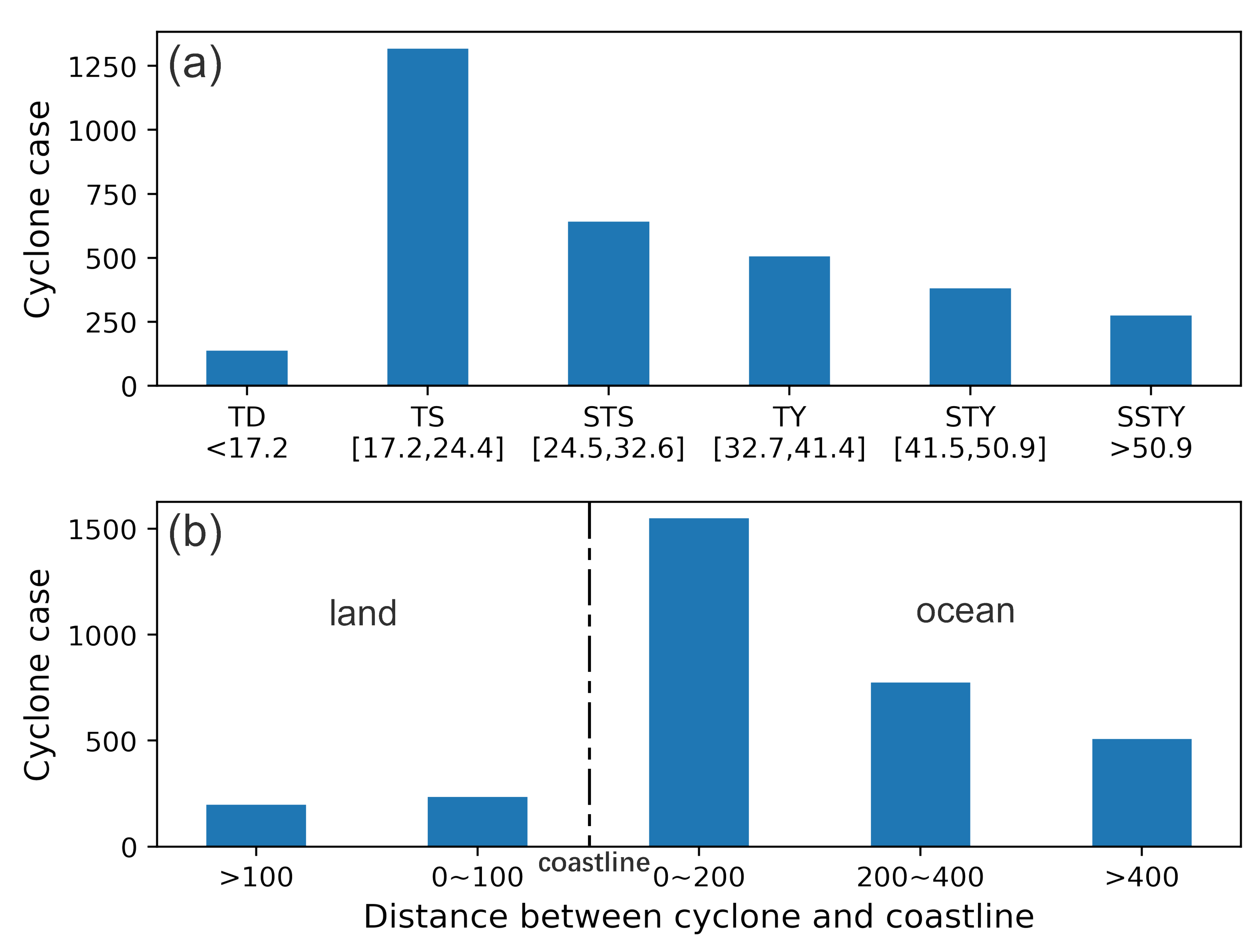
The satellites in the Himawari series are the first geostationary meteorological satellites that were launched by the Japan Meteorological Agency in 1977. H-8 is a new generation of the Himawari series that was launched in October 2014 and became operational in July 2015 [33,34]. H-8 has 16 observation spectral bands with spatial resolutions of 0.5 or 1 km for visible and near-infrared bands and 2 km for infrared bands. The observation area is 60S–60N, 80E–160W, covering the majority of the western North Pacific basin and providing images at temporal and spatial resolutions of 10 min and 5 km, respectively. In the current study, five H-8 L2 cloud products from the years 2015 to 2020 are used, including cloud optical thickness (CLOT), cloud top temperature (CLTT), cloud top height (CLTH), cloud effective radius of band-6 (CLER), and cloud type (CLTY). Visually, the TC structure that is well captured by these products is highly related to TC intensity. Therefore, using a DL-based model to perform some computer vision tasks to aid in TC intensity estimation is feasible and worthwhile. This study only examines the usage of H-8 L2 cloud products in daytime TC intensity estimation tasks due to the unavailability of nighttime observations.

2.2. TC Data

The TC dataset is derived from the real-time typhoon track system released by the Department of Water Resources of Zhejiang Province, data from which are available each three-hour period for pelagic TCs and for every one-hour period for inshore TCs. It contains detailed TC tracks and their associated time, longitude, latitude, minimum sea level pressure, maximum wind speed (sustained 2 min average wind speed), moving direction, moving speed, and landfall site over the western North Pacific basin. In order to match the time span of the five cloud products mentioned above, a total of 3264 original TC records (from 147 typhoon cases from the years 2015 to 2020) were extracted. For brevity, the maximum wind speed was used as the target TC intensity, which is also the labeled variable for the intensity regression task below. According to the TC intensity classification criteria by the China Meteorological Administration (note that the criteria is different from the Saffir–Simpson criteria), six TC types are defined: tropical depression (TD), tropical storm (TS), strong tropical storm (STS), typhoon (TY), strong typhoon (STY), and super strong typhoon (SSTY) (see Figure 1a). To facilitate the analysis below, these TCs are also divided into landfall TCs and non-landfall (nautical) TCs based on their distances from the coastline (see Figure 1b).

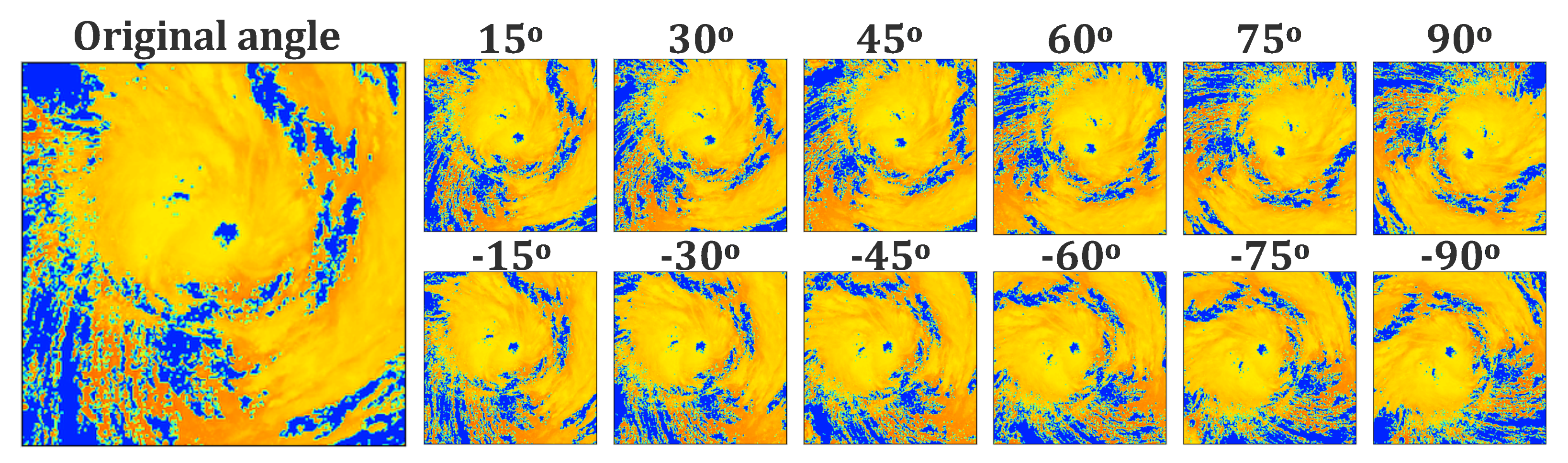
2.3. Data Augmentation

Training a DL model usually requires an enormous amount of data; hence, we utilized the data augment technique to expand the initial samples. For example, Figure 2 shows the data augmentation performed on the CLTT cloud product. For each image, a total of 13 different images (side length: 1280 × 1280 km) are generated at +/−15 degree rotational increments and are positioned at the same storm center (longitude and latitude), resulting in an array that is 13 × 256 × 256 in shape. The CLOT, CLTH, CLER, and CLTY products are collected in a similar way. Therefore, the final sample size is 42,432 × 5 × 256 × 256. Note that H-8 is unable to conduct monitoring activities at night because it uses visible bands, and there are also some abnormal data due to hardware failures, so the final sample size was reduced from 42,432 to 39,787.

2.4. Convolutional Neural Network (CNN)

The detailed mathematical principle and formula derivation of the CNN are presented in studies [39,40]. A CNN consists of three key layers: convolutional (feature extraction) layers, pooling (down sampling) layers, and dense (fully connected) layers. In the convolutional layers, various trainable convolutional kernels (also known as filters) with a constant size have the “parameters sharing” (weights and biases) feature, which enables them to extract multiple features from the original input pattern. This step not only reduces the computational cost and the number of parameters, but it also alleviates over-fitting to some extent. Pooling layers are usually inserted among consecutive convolutional layers, retaining the main features as well as reducing the number of parameters. As such, they can reduce the dimensionality of the representation, and create an invariance to small shifts and distortions [24], which helps to increase the generalization ability and to alleviate the over-fitting of the model. The flexible combination of convolutional layers and pooling layers may extract some well-organized features from the original inputs. Dense layers act as classifiers or regressors in the CNN architecture; in other words, the outcomes of convolution and pooling can be integrated by the dense layers. The CNN method is well suited for image processing and pattern recognition, especially for images with translational invariance, rotational invariance, and scale invariance. Because TC images are generated under 13 rotational angles, are always centered on the storm center (see Figure 2), and usually have well-organized structures (e.g., outer wind bands, middle spiral cloud bands, cyclone eye walls, inner cores) with various shapes and sizes, it is possible to assume the three invariances mentioned above. Using the regressive pattern of the CNN, the TC intensity estimation from satellite cloud products (seem as images) can thereby be converted to a nonlinear feature extraction problem. The basic architecture of the CNN follows the net from the “Oxford Visual Geometry Group (hereafter VGG; [41])”, which is a widely used technology in computer vision tasks. The VGG in this study contains four “convolutional blocks” with filter sizes increasing from 32 to 256 (see Figure 3).

2.5. Residual Learning

Intuitively, the VGG architecture extracts ample features by stacking multiple convolutional and pooling layers. However, an architecture that is this deep can raise three issues: the huge consumption of computing resource, model over-fitting, and model gradient vanishing/exploding [42,43]. The above issues can be solved by a graphic processing unit (GPU) cluster, expanding the sample size, implanting regularization layers, etc. In practical training processes, stacking more layers will inevitably lead to network degradation that is not caused by over-fitting [38,44]. Therefore, [38] presented a deep residual learning framework, suggesting the utilization of a few stacked layers to fit a residual mapping from an initial mapping instead of directly fitting an initial mapping. Such deep residual learning can be implemented by a feedforward network with shortcut connection and can thus be embedded into the VGG architecture flexibly. Notably, residual learning helps to accelerate convergence. This study will embed “double-level” residual learning (see Res1 and Res2 in Figure 3) in the VGG architecture.

2.6. Attention Mechanism

Note that the importance of each cloud product (channel) will not be sorted before the convolutional operation in the VGG architecture. Moreover, for each cloud product, values at different areas (e.g., TC eye, TC eye wall, TC outer spiral rain-band) will play divergent roles within convolutional operation. The above conjectures imply that appending an “attention mechanism” in the VGG architecture would obtain much stronger representation power. Simply, the attention mechanism makes the architecture pay more attention to the “what” and “where” of the cloud products. Ref. [37] proposed a convolutional block attention module (CBAM) containing two independent modules: channel attention and spatial attention. CBAM sequentially estimates attention sequences along the channel and spatial dimensions, uses inner product operation to integrate the attention sequences and the raw input features, and further obtains adaptive feature refinement, and can hence be seamlessly implanted into the VGG architecture. The CBAM in this study can further enhance feature representation for the VGG architecture, help the network focus on significant “feature maps”, and inhibit unnecessary ones among the convolutional layers.

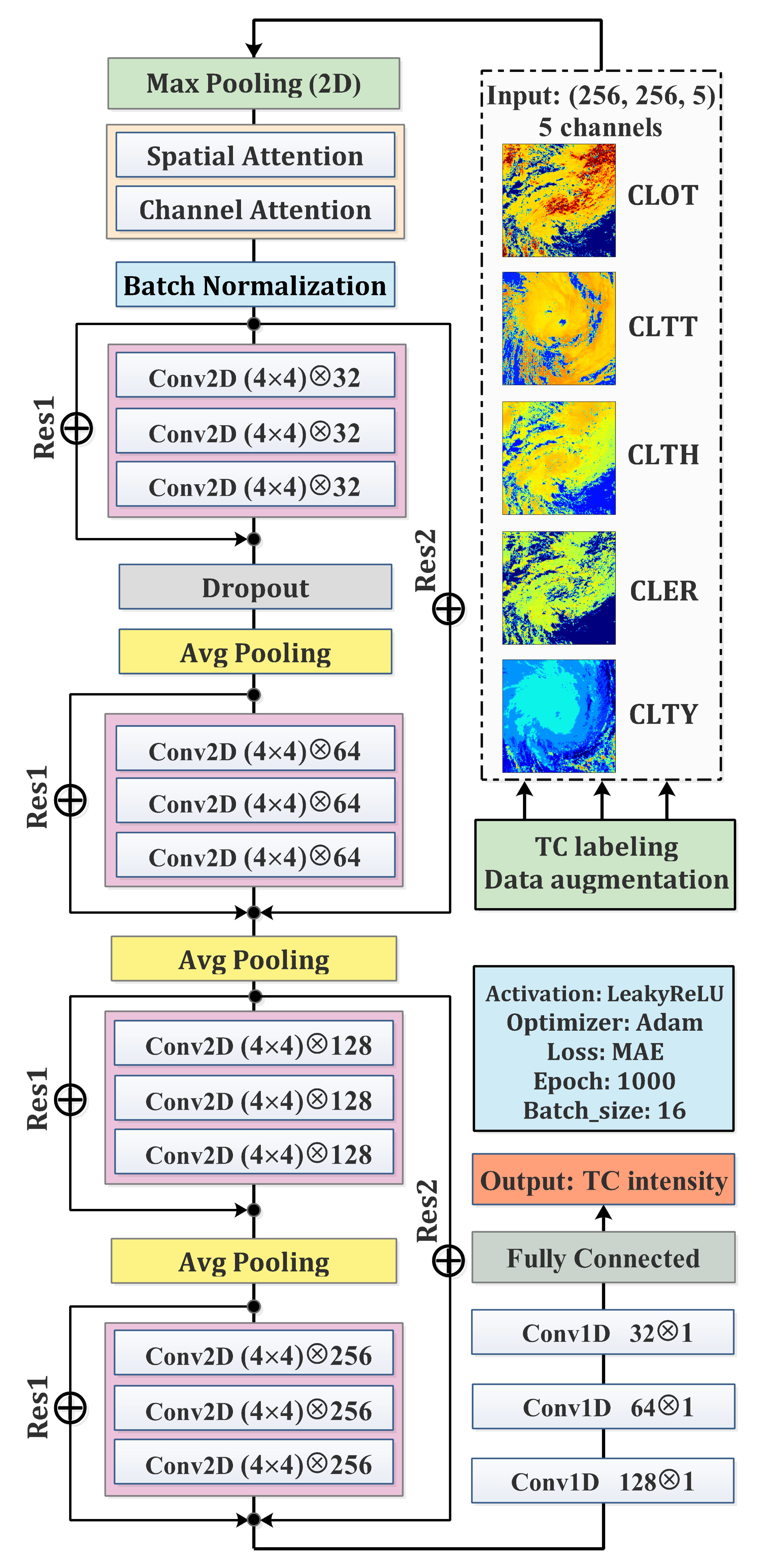
2.7. The Framework of TC Intensity Estimation Model

In summary, the complete TC intensity estimation model consists of residual learning and CBAM based on the VGG architecture, as shown in Figure 3. In the model, the maximum pooling layer is added before feeding the input data into the training process, and then CBAM is carried out at the backend of the maximum pooling layer. The first residual learning level (Res1) is added at each convolutional module (and includes three convolutional layers); the second residual learning level (Res2) is used for identity mapping and connects the first and the second convolutional module as well as the third and the fourth convolutional module to each other. The average pooling layer is performed ahead of each convolutional module. Note that after all of the convolutional modules, we use several 1-D convolutional layers and one fully connected layer rather than one single dense layer to fully connect the training labels. Such an operation will help to reduce the number of parameters. The last layer releases the estimated TC intensities which are one-to-one correspondences to the training labels (target intensities). Moreover, we also adopted a “Batch-Normalization” layer and a “dropout” layer to ease over-fitting. All of the convolutional layers (Conv2D) have leaky rectified linear unit (LeakyReLU) activation functions, and all of the related kernel sizes are $4\times 4$, the strides are all set to $(1,1)$, and their padding strategies are all set to “same”, with their kernel numbers being 32, 64, 128, and 256. The kernel size of the 1-D convolutional layers (Conv1D) decreases from 128 to 32. Model training and optimization were performed using the adaptive momentum (Adam) gradient descent optimizer and mean absolute error (MAE) loss function. The total number of training epoch is 200, and the number of the early stopping epoch is 20, which helps to alleviate over-fitting. Therefore, the input size is (256, 256, 5), while the output size is 1 (scalar TC intensity determined by the model).

For model configuration, the modeling samples (sample length is 39,798) were divided into two parts: the cross-validation set (first 90%, 35,808 samples) and the independent test set (last 10%, 3979 samples). Specifically, the cross-validation set was further divided into six equal groups (each group has 5968 samples), and the six-fold cross-validation method was used to tune the model’s trainable parameters during the training process, which means that we trained the model six times using different parameters and validation losses, ensuring each sample was validated one time. The above steps can be implemented through the “Tensorflow” package in Python syntax. To further examine the model’s generalization ability, we tested the model two times (which have the two lowest validation losses from the previous cross-validation step) using independent test sets and averaged their outputs.

3. Results

3.1. Assessment on Cross-Validation Data

Here, we analyze the dependability of the model using the cross-validation set. We adopted the DL architecture with CBAM and Res1 (see Section 2.7 and Figure 3) to perform the assessment. Figure 4a compares the estimated intensity $\left(\widehat{y}\right)$ and target intensity $\left(y\right)$ in 4 m/s intervals and shows the probability of the estimated $\widehat{y}$ conditional on target y. Intuitively, the linear fitting suggests that $\widehat{y}$ is highly correlated with y through $\widehat{y}=0.79\times y+5.48$ $(R^2=0.95)$. The model demonstrates the overestimation of the intensity at $y<24$ m/s, showing with high probabilities, especially for those at the 14 m/s intervals and that have a probability close to 1. Comparatively, TCs with intensities exceeding 30 m/s intervals were underestimated by the model at various probability levels, and the biases increased with the intensity. The largest underestimation occurred for violent TCs with intensities close to 60 m/s. Considering the fact that the intensity of most TCs are around 30 m/s (see Figure 1), the biases in estimating those marginal TCs (e.g., tropical depressions or typhoons, strong typhoons) are considered acceptable. These results are consistent with the findings of [27].

Moreover, we calculated the standard deviation $\left(\sigma \right)$ of the estimated intensity to investigate the model’s stability. In Figure 4b, the standard deviation is lower than 1.6 m/s when $y<40$ m/s and then gradually increases with y, reaching its peak at $y=56$ m/s. Overall, the standard deviations are fairly low, with values ranging in 1–2 m/s, suggesting that the model is relatively stable in reproducing different TC intensities, especially for those of weak TCs. Figure 4c presents the bias and the RMSE of the estimated intensities. It is clear that the biases are negatively correlated with the target intensities, where overestimations appear in weak TCs (tropical depressions, tropical storms), with bias values ranging from 0–2 m/s, and underestimations occur in strong TCs, with biases ranging from −9 to 0 m/s. Generally, the RMSE values are within the small range (<7 m/s), suggesting that the designed architecture and parameters are effective for model training. Consistent with the bias values, the model demonstrates small RMSEs at $y<32$ m/s intervals but begins to degenerate as the target intensities increase. The possible reason for such large biases in strong TCs could be due to the relatively small set of samples (e.g., strong typhoons and super typhoons in six typhoon seasons) are used for feature extraction.

Figure 5 presents a boxplot of the estimated biases at different regions. Overall, the estimated biases range from −10 to 4.5 m/s. Though most TCs are overestimated by the model, the mean biases are around 0 m/s, revealing that overestimation almost reaches parity with underestimation. Compared to nautical (non-landfall) TCs, the biases from landfall TCs have smaller fluctuations. Note that most landed TCs end with low intensities, and these weak TCs account for the small biases for low intensity TCs discussed above. For nautical TCs, according to the shape of each group box, it is obvious that pelagic TCs (D > 400 km cyclones) have greater biases than inshore TCs (0 < D < 200 km and 200 < D < 400 km cyclones), indicating that the estimated biases increase as the coastal distances increase. Because most TCs are recorded more frequently (1-h sampling) over inshore areas than they are pelagic areas (3-h sampling), our model can excavate useful information and can fit the target intensities with relatively small biases by using these ample training samples of inshore TCs.

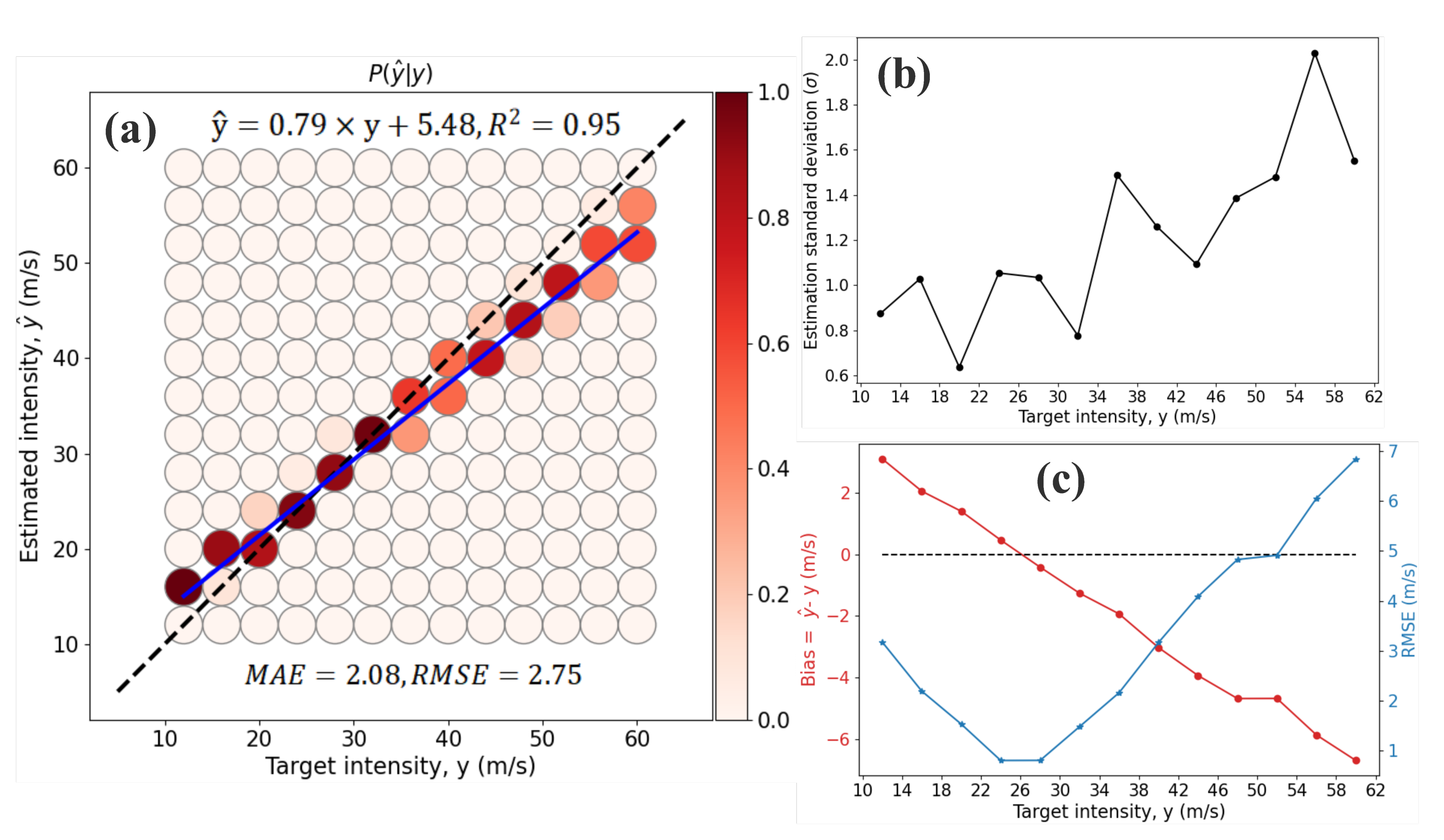
3.2. Performance on Independent Test Data

We verified the performance of the model using an independent data set. As shown in Figure 4, several statistics are calculated. Overall, the estimated intensity $\widehat{y}$ matches with the target y with a liner fitting of $\widehat{y}=0.84\times y+4.15$ $(R^2=0.85)$, which is slightly inferior to that in the cross-validation data. In Figure 6, it is clear that overestimations appear in $y<20$ m/s TCs with relatively high probabilities. In contrast, underestimations can be found in the $y>30$ m/s TCs with various probabilities. For example, $y\approx 48$ m/s TCs are predicted by the model to have an intensity 44 m/s with probability of 0.5, and $y\approx 50$ m/s TCs are underestimated at intensity of 46∼50 m/s with low probabilities. Nevertheless, the model is still able to reproduce maximum intensities (at around 50 m/s). Similar to previous assessment on cross validation data, our trained model has a tendency to overestimate (underestimate) TC intensities when the target intensity is low (high). This is not surprising, since the loss function of our model is MAE and could be generally minimized by providing the mean TC intensity outputs. However, in view of the small MAE and RMSE (both are slightly greater than that from validation data) values, the model is skillful in predicting the TC intensity.

To conduct a comprehensive performance analysis, we also compared the proposed model against those developed in other existing studies. The RMSE is presented in

Table 1. Comparison with existing studies.

Model/Method	Satellite Data/Channel	RMSE (m/s)	Reference
ADT	IR, visible/PMW imagery	5.77	[45]
DAV	GOES-12, IR (10.7 µm)	6.68	[46]
DAVT	MTSAT, IR (10.7 µm)	6.55	[22]
DeepMicroNet	DMSP, TRMM, Aqua AMSR-E etc.	4.93	[25]
CNN-TC	GridSat, IR1, WV, PMW	4.31∼4.52	[26]
2D-CNN, 3D-CNN	COMS MI, IR1, IR2, WV, SWIR	4.27∼5.82	[14]
TCICENet, TCICENet-S	GMS, GEO, MTSAT, H-8, etc.	4.42∼4.93	[13]
VGG-ResNet-CBAM	H-8 L2 cloud products	4.06	This study

since it was used as the evaluation indicator in these existing studies. ADT [45] has many enhancements compared to its previous version and is used operationally by TC forecast centers worldwide. However, it depends on the comprehensive application of multi-source data, as well as objective analysis. The authors of [22,46] used the DAV technique and infrared imagery to estimate TC intensity in the north Atlantic and the eastern North Pacific basins, achieving RMSEs of 6.68 m/s and 6.55 m/s, respectively. The relatively high RMSE values that were achieved by the DAV are probably caused by DAV signal oscillations that do not occur in smoothed best track intensity estimates. The CNN-based methods adopted various satellite images as input and achieved satisfactory performance. For example, the RMSE ranges from 4.31 to 4.52 m/s in [26] and from 4.42 to 4.93 m/s in [13]. The author of [14] utilized both 2D-CNN and 3D-CNN, and the the minimum RMSE was reached at 4.27 m/s. In [25], the “DeepMicroNet” model achieved an RMSE of 4.93 m/s compared to the reconnaissance-aided best track intensity. Although the above CNN-based methods outperform the DAV and ADT in terms of the RMSE, they extract nonlinear features by blindly stacking multiple convolution layers, which may be affected without the interrelations of each feature and may introduce intensity estimation errors. Note that by using residual connections and an attention mechanism, our model extracts and reorders potential features more effectively, obtaining an RMSE as low as 4.06 m/s, which is considered to be a satisfactory and comparable result.

4. Discussion

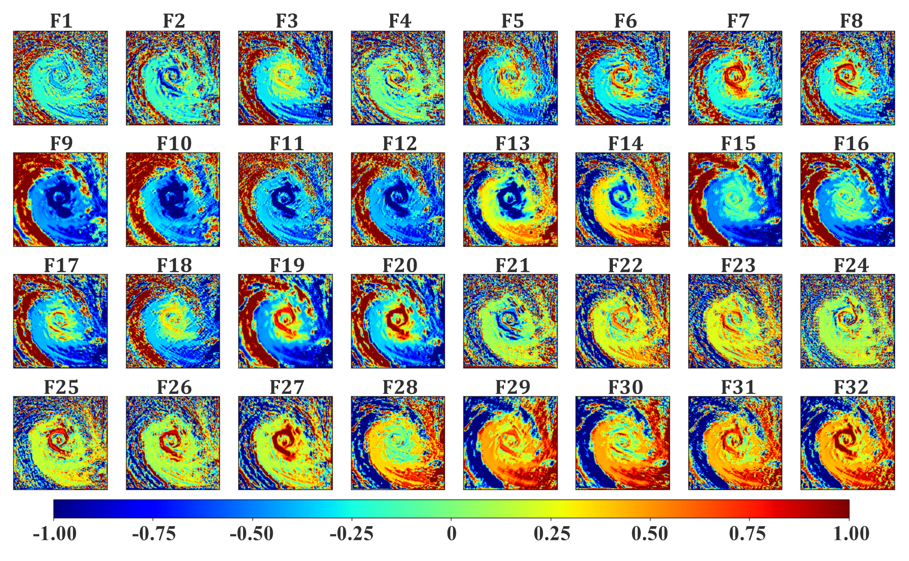
4.1. Interpretability of the Model

Similar to most DL methods, our model is also an “end-to-end” black box that is unable to interpret the estimated results. Here, we use a so-called “feature map” to address this disadvantage. It is known that convolution kernels (filters) are the main operators for feature extraction in a CNN-based architecture; thus, we visualized the outputs from the kernels of one convolutional layer to intuitively understand and interpret the forward process of the model. Figure 7 exhibits 32 feature maps derived from the convolution process of the first “Conv2D” layer (with a total of 32 filters). From Figure 7, we can recognize various TC structures and related cloud band features directly. For example, F1∼F10 describe the formation stages, development stages, and whirling patterns of TC eye wall cloud bands. In terms of the outer wind bands and the middle spiral cloud bands in F1∼F10, their shapes appear to be amorphous, presumably because (1) the CBAM assigns distinct spatial attentions to them and (2) the various filters activate all of the pixels differently. There are conspicuous outer wind bands and middle spiral cloud bands framing F9∼F12 that have very high negative pixel values. The model seems to focus on outer wind bands and TC eye wall bands while disregarding those marginal clouds (clouds around the edge of a storm) in F13∼F14, in the opposite of which is observed in F15∼F16. Moreover, F21∼F27 also depict the intensification of middle spiral cloud bands and the storm’s inner core structures, and F28∼F32 pay more attention to the outer wind bands. All of above feature maps record the storm’s spiral patterns and symmetric structures exactly.

As CBAM is used in our model, it is important to determine how the feature maps are activated by the five channel inputs (cloud products) and whether they act as further indicators for cyclone intensity estimation. For example, the feature maps in F6∼F8, F19∼F20, F25∼F27, and F31∼F32 show TC eye wall bands and inner core structures that are associated with CLOT and CLTH; the feature maps in F15∼F16 have outer wind bands that are associated with CLTT and CLTY; the feature maps in F1∼F5 and F21∼F24 depict marginal clouds that are associated with CLTH and CLTY; and the feature maps in F13∼F14 have TC eye wall bands and outer wind bands that are likely associated with CLTH and CLER, etc. Overall, it is hard to elaborate a direct link between each feature map and each single cloud product due to various attentions that the CBAM pays to each input. However, these diverse feature maps enable the model to represent complex aspects of TC intensity.

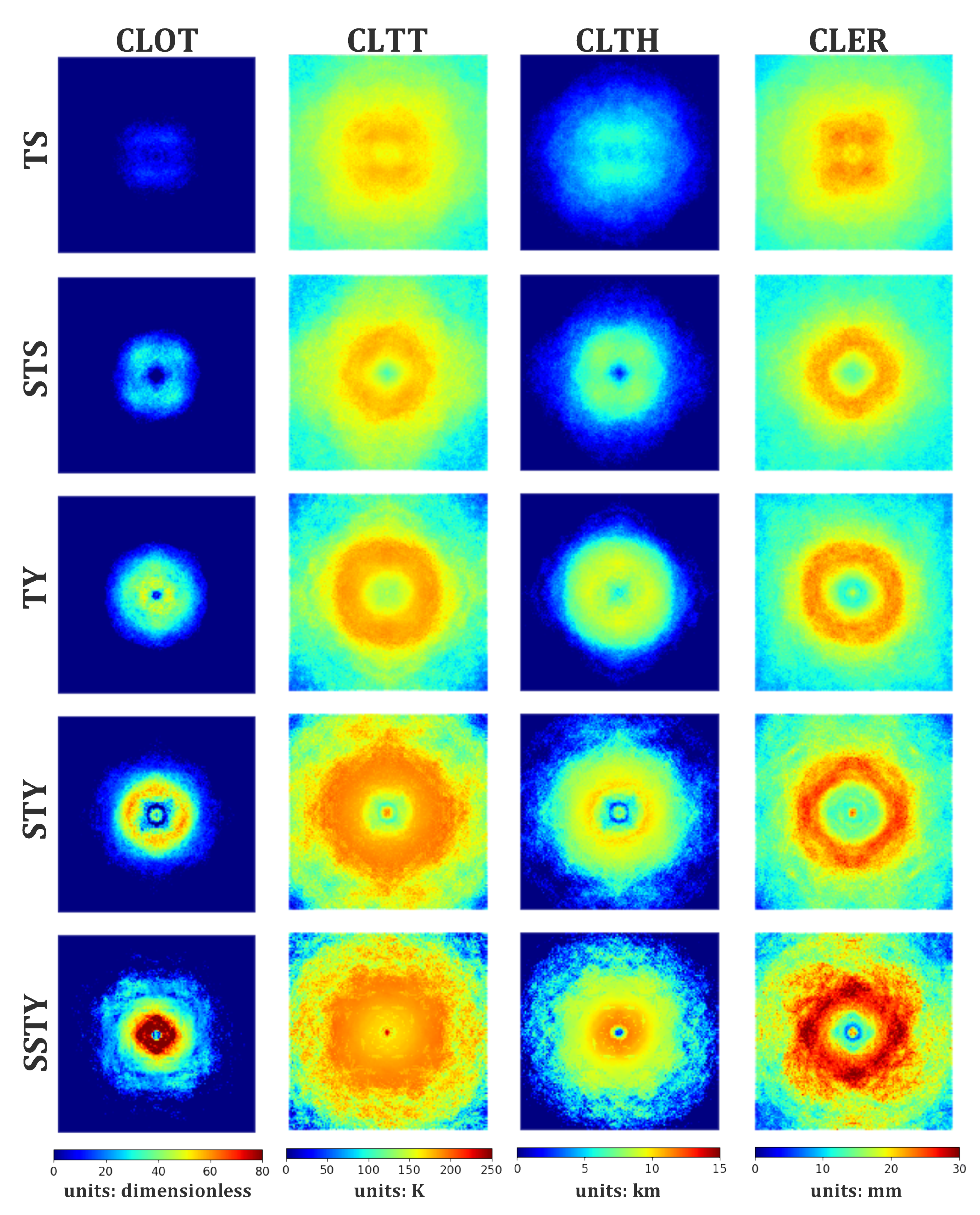
4.2. Initial Cloud Products under Different TC Intensities

Because our model uses five cloud products as the training inputs, it is important to comprehend how these products work when estimating TC intensities. It is well known that TC intensities are affected by many aspects, such as the size, structure, warm moist air, convergence on the upper troposphere, divergence on the lower troposphere, convective activity, wind shear, orographic effects, etc. [47,48,49,50,51]. In the visualized cloud products, the well-organized structure of the cloud system and the decentration between convective activity and the center of the TC are two important dynamic factors that reflect the strength of the vorticity and vertical wind shear, respectively. In addition, the cloud type and the cloud top temperature are two key thermal factors that reflect the development of convective activity and the development of the TC’s inner core, respectively. Figure 8 shows initial cloud products for TCs with different intensities than those observed in the independent test dataset.

Obviously, the TC intensity increases as the CLOT increases. In particular, there are conspicuous spiral cloud bands in STY and SSTY when the CLOT is greater than 60 and 100 (unit: dimensionless), respectively. Additionally, empty areas (no clouds) can be found around storm eyes. From TS to SSTY, the cloud systems become much more highly organized (see CLOT, CLTH and CLER). The above analysis agrees with our background knowledge that outer wind bands and spiral cloud bands might gather abundant warm moist air and convective clouds, which intensify convective activities and produce TCs. Additionally, from TS to SSTY, the values of both CLOT and CLTH become higher, indicating the development of convective activity and the inner core of a TC. Generally speaking, CLTT and CLTH are closely related to updraft and are indirectly related to TC intensity. In the troposphere, stronger updrafts are more prone to lifting convective clouds to the top, causing the cloud top temperature to decrease. Occasionally, however, strong updrafts do not lead to strong TCs due to the inhibition of anticyclones at high-level divergence. Considering that convective activities mainly occur in the areas between the outer of TC eye wall and the spiral cloud band, it is not surprising that low CLTT but high CLTH values are centered in such areas, especially those areas in strong TCs, such as in TY, STY, and SSTY. Moreover, The eyes of TCs can be found in the CLTH of STS and SSTY, since downdrafts prevail around TC centers. In terms of CLER, it can reflect moist air conditions to some extent. From weak TCs to strong TCs, the convective activities become stronger, while their ring-like CLER values become more evident. This proves once again that strong convective activity mostly takes place in the areas between the outer TC eye wall and the spiral cloud band.

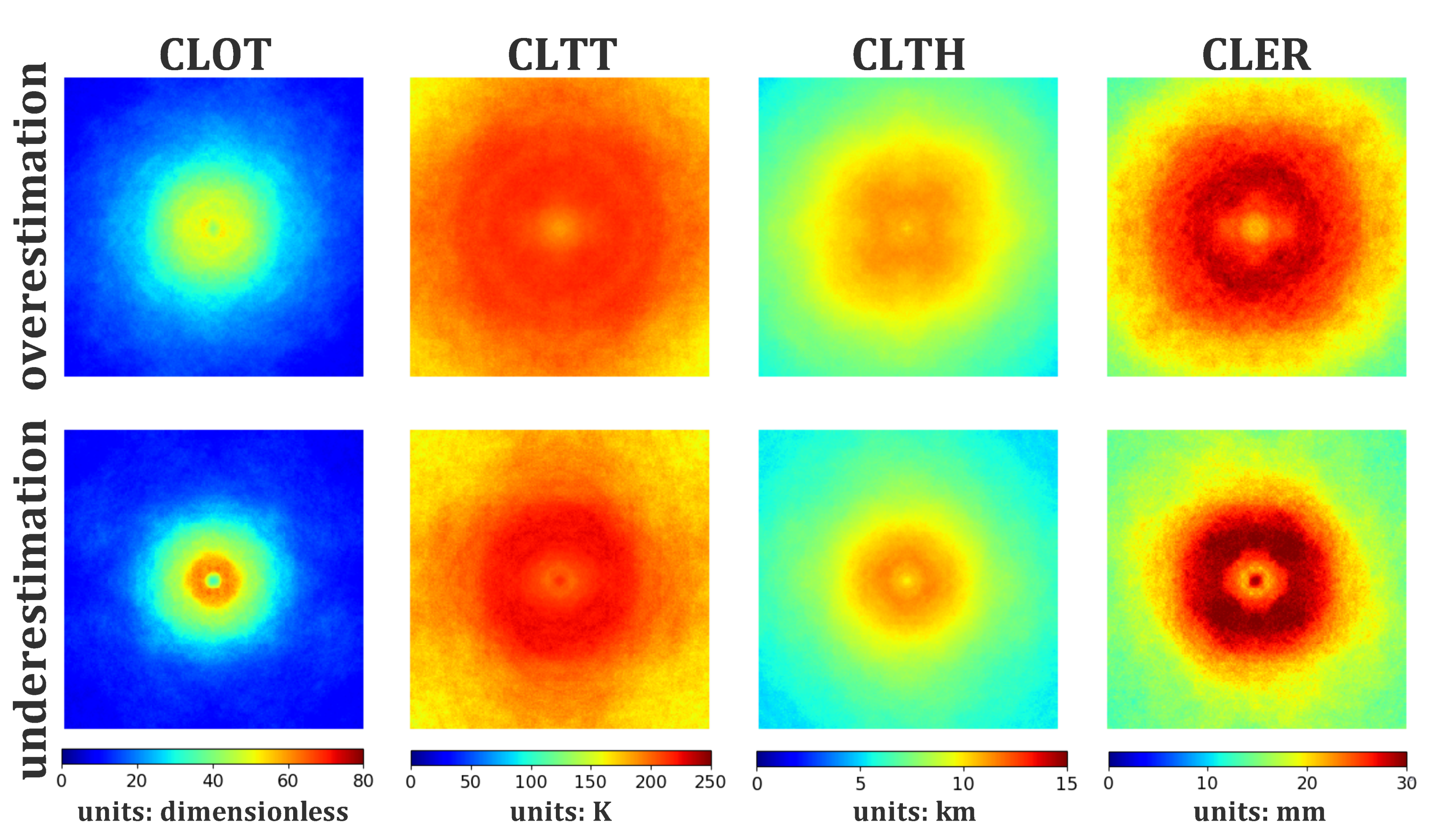
4.3. Cloud Product Composites on Overestimation and Underestimation

Here, we used cloud product composites to understand the model prediction behavior (overestimation or underestimation). Figure 9 demonstrates the composites of four cloud product channels from the independent test data. Intuitively, the underestimation cases correspond to more vivid cloud products compared to overestimation cases. Different cloud band outlines and inner cores of the storms are distinguished (especially for CLOT, CLTH, and CLER) in the underestimation cases, but are not in the overestimation cases. Overall, the underestimated TCs have deep and well-organized cloud system structures, and the inner core structures are clear, which is the opposite in the overestimated TCs, suggesting that the estimated TC intensity is highly related to the analog convective activity and the inner core of the TC. According to the analysis in Section 4.2, most overestimations (underestimations) occur in weak (strong) TCs, which correspond to vivid (assorted) cloud products. The model’s performance is highly affected by initial cloud products.

4.4. Further Discussion on the Model’s Architecture

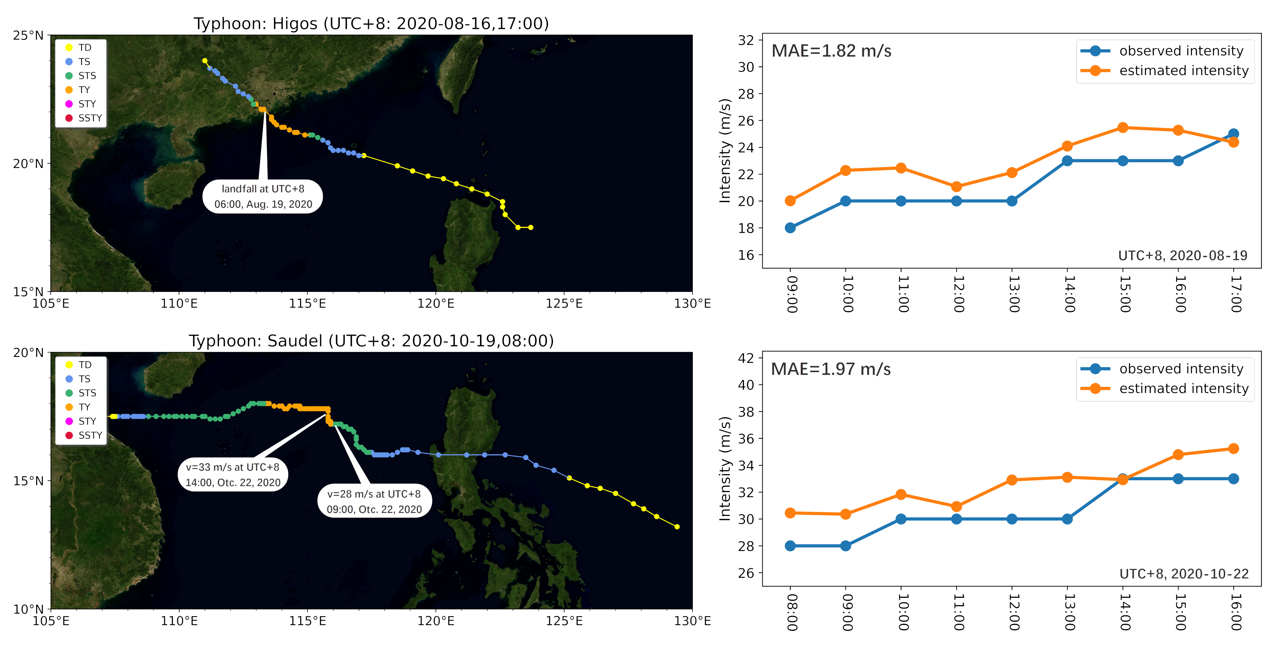
The model’s architecture consists of a VGG network, residual learning, and CBAM. To further illustrate the necessity of the designed architecture, we implemented several controlled experiments (

Table 2. Comparison of several DL architectures. Note: CA = channel attention; SA = spatial attention; CBAM = CA + SA; Res1 and Res2 are two kinds of residual learning modules, such as those shown in Figure 3. The running time is counted over one training epoch; the fifth architecture (VGG + CBAM + Res1) with smallest MAE and RMSE is adopted by this study. All of the above experiments codes are performed on the following environment: Python = 3.8, tensorflow = 2.4.1, GPU = NVIDIA GeForce RTX 3090 with 24G video memory.

Architecture	Num. of Parameters	Running Time (s)	MAE (m/s)	RMSE (m/s)
VGG	3,478,241	138	3.62	4.62
VGG + CA	3,478,257	136	3.61	4.53
VGG + SA	3,478,260	145	3.81	4.80
VGG + CBAM	2,789,700	78	3.40	4.29
VGG + CBAM + Res1	301,444	114	3.23	4.06
VGG + CBAM + Res2	844,932	67	3.57	4.43
VGG + CBAM + Res1 + Res2	2,929,220	126	3.38	4.25

). As seen from the first three experiments, both VGG + CA and VGG + SA have roughly the same number of parameters as that of VGG, with VGG + SA having the longest running time. In terms of the MAE and RMSE, VGG + CA is marginally superior to VGG, while VGG + SA produces a greater MAE and RMSE than VGG and VGG + CA do. The above results demonstrate that the estimation performance is only slightly improved when appending a channel attention module to the basic VGG but that it degrades when appending the spatial attention module, indicating that the channel attention mechanism is more effective than the spatial attention mechanism. This is presumably because the former concurrently derives “average pooling” and “maximum pooling” to determine which feature (upon channel axis) is more important, while the latter might make up for the deficiency of the former by determining “where” the operator should focus within each feature. Therefore, we can state that when using both the spatial and channel attention modules (VGG + CBAM), the MAE and the RMSE reduce to 3.40 m/s and 4.29 m/s, respectively, and the running time even decreases almost one time.

Another interesting finding from the last three architectures in Table 2 is that different “skip connecting modes” performed differently. Res1, which connects only one convolutional block (VGG + CBAM + Res1), is superior to Res2, which connects two convolutional blocks (VGG + CBAM + Res2); although Res1 has a longer running time than Res2, the number of parameters is substantially reduced; furthermore, both the MAE and RMSE in Res1 are smaller than those in Res2. These phenomenon can be explained by the network degradation effect. In a VGG network, based on the principle of “Data Processing Inequality”, as the layer increases, some of the useful information included in the feature maps gradually decreases. However, adding more residual learning modules (which can be considered as an “identity mapping” process) will help the structure to retain more useful information on each feature map; hence, when a skip connects longer steps, than less running time is required than when a skip connects shorter steps, such as in Res2 versus Res1. Additionally, note that, for a deep VGG network, the weights in some layers or nodes are too small, subtly impacting the architecture. Therefore, adding appropriate residual learning modules (which can be considered as a “pruning” process) will help to detach the number of parameters in the back propagation of gradients and will further compress the architecture. Hence, it is not hard to understand that Res2 occupies more parameters than Res1 but that it also produces a greater MAE and RMSE. Furthermore, if Res1 and Res2 are used concurrently (VGG + CBAM + Res1 + Res2), then the model only demonstrates slight improvement compared to when Res2 (VGG + CBAM + Res2) or CBAM (VGG + CBAM) are used alone. However, no improvement is observed when Res1 (VGG + CBAM + Res1) is used alone. The above results suggest that residual learning blocks are favorable for saving computational cost and for improving estimation performance. However, it does not necessarily mean that some mindless residual learning modules would provide better TC intensity estimations.

4.5. Case Study

Here, we choose two representative typhoon cases to examine the performance of the model (Figure 10). The first typhoon, Higos, was generated on 16 August 2020 and made landfall in southern Zhuhai at about 6:00 a.m., 19 August 2020. It was rapidly downgraded to a strong tropical storm (STS) after 9:00 a.m. and then moved northwestwards at a speed of 25 m/s. This typhoon caused huge losses over a short period of time. Our model slightly overestimated the storm’s intensity (after landfall), with an MAE of 1.82 m/s, agreeing well with the fact that the model has a tendency to overestimate TC intensity when the target intensity is low (e.g., less than 30 m/s). The development after landfall is well captured. The second typhoon, Saudel, was generated on 19 October 2020, and its intensity increased from 28 m/s (at 09:00 a.m., 22 October) to 33 m/s (at 14:00 p.m., 22 October) and was judged as a rapid intensification typhoon (+5 m/s per 6-h). Our model successfully captures its intensification feature with an MAE of 1.97 m/s. Note that though the model generally tends to underestimate the TC intensity when the target intensity is high, for Saudel, it was slightly overestimated.

5. Conclusions

In this study we propose a DL-based model for TC intensity estimation using the H-8 L2 cloud products CLOT, CLTT, CLTH, CLER, and CLTY. The model uses VGG as the basic architecture and integrates “attention mechanism” and “residual learning” to reduce the number of parameters as well as to improve the estimation precision. The model was trained and optimized under six-fold cross-validation data and was further evaluated using independent test data. The following useful conclusions can be drawn:

(a) For cross-validation, the model behaves differently for different TC intensity intervals. Generally, underestimation is seen in strong TCs, and overestimation is observed in weak TCs. Over specific regions, biases in estimated intensities for landfall TCs have smaller fluctuations than those for nautical TCs due to the imbalance in the recorded TC samples, which may affect the model’s training and feature representation. For the independent test, our model produced a relatively low RMSE of 4.06 m/s and an MAE of 3.23 m/s, which are comparable to those determined from existing studies using Dvorak-based techniques and various other CNN-based DL techniques.

(b) By visualizing the outputs from one of the convolutional layers, we were able to clearly identify various cloud organization patterns, storm whirling patterns, and TC structures, which helped the model represent the complex changes in the TC intensity and produce reliable estimations. Moreover, the initial cloud products were able to reflect some of the factors associated with TC intensity, such as warm moist air, convergence, divergence, and convective activity. Furthermore, by examining the initial cloud products under different intensity levels, we were able to determine that our model has a tendency to overestimate (underestimate) weak (strong) TCs. Finally, the superiority of the model designed in this paper is demonstrated through a comparison with other residual learning and CBAM-based architectures.

Overall, the proposed DL-based model is promising for TC intensity estimation and future studies are highly needed to improve the model further. First, more satellite imagery from different infrared bands, microwave bands, regions, and nighttime periods, as well as TC best track data, ground, marine, and voyage observations should all be considered to augment the model’s training samples [14,25,31] in order to improve the robustness of the model. Second, because the TC intensity is affected not only by its size and structure but also by ambient thermodynamic conditions and physical factors [52,53], future work should consider more parameters such as surface temperature, water vapor, sea level pressure, vertical wind shear, steering flow, etc. Third, the proposed architecture is tackled as a feature extraction and regression task intended for TC intensity estimation. More DL architectures (e.g., ConvLSTM, [54]) can be tried for spatial-temporal series regression tasks in TC tracks or precipitation nowcasting in the future.

References

1. Tang, D.L.; Sui, G.; Lavy, G.; Pozdnyakov, D.; Song, Y.T.; Switzer, A.D. (Eds.) Typhoon Impact and Crisis Management; Springer: Berlin/Heidelberg, Germany, 2014; pp. 1–578. [Google Scholar]
2. Davis, C.A. Resolving tropical cyclone intensity in models. Geophys. Res. Lett. 2018, 45, 2082–2087. [Google Scholar] [CrossRef]
3. Pamela, P.; Chiara, P.; Alessandro, A.; Stefano, P.; Annett, W. Tropical Cyclone ENAWO—Post-Event Report. 2017. Available online: https://publications.jrc.ec.europa.eu/repository/handle/JRC108086 (accessed on 31 January 2022).
4. Courtney, J.B.; Langlade, S.; Sampson, C.R.; Knaff, J.A.; Birchard, T.; Barlow, S.; Kotalg, S.D.; Kriat, T.; Lee, W.; Pasch, R.; et al. Operational perspectives on tropical cyclone intensity change part 1: Recent advances in intensity guidance. Trop. Cyclone Res. Rev. 2019, 8, 123–133. [Google Scholar] [CrossRef]
5. DeMaria, M.; Sampson, C.R.; Knaff, J.A.; Musgrave, K.D. Is tropical cyclone intensity guidance improving? Bull. Am. Meteorol. Soc. 2014, 95, 387–398. [Google Scholar] [CrossRef] [Green Version]
6. Kim, S.H.; Moon, I.J.; Chu, P.S. Statistical–dynamical typhoon intensity predictions in the western North Pacific using track pattern clustering and ocean coupling predictors. Weather Forecast. 2018, 33, 347–365. [Google Scholar] [CrossRef]
7. Leroux, M.D.; Wood, K.; Elsberry, R.L.; Cayanan, E.O.; Hendricks, E.; Kucas, M.; Otto, P.; Rogers, R.; Sampson, B.; Yu, Z. Recent advances in research and forecasting of tropical cyclone track, intensity, and structure at landfall. Trop. Cyclone Res. Rev. 2018, 7, 85–105. [Google Scholar]
8. Judt, F.; Chen, S.S. Predictability and dynamics of tropical cyclone rapid intensification deduced from high-resolution stochastic ensembles. Mon. Weather Rev. 2016, 144, 4395–4420. [Google Scholar] [CrossRef]
9. Zhao, Y.; Zhao, C.; Sun, R.; Wang, Z. A multiple linear regression model for tropical cyclone intensity estimation from satellite infrared images. Atmosphere 2016, 7, 40. [Google Scholar] [CrossRef] [Green Version]
10. Zhuge, X.Y.; Guan, J.; Yu, F.; Wang, Y. A new satellite-based indicator for estimation of the western North Pacific tropical cyclone current intensity. IEEE Trans. Geosci. Remote Sens. 2015, 53, 5661–5676. [Google Scholar] [CrossRef]
11. Shimada, U.; Sawada, M.; Yamada, H. Evaluation of the accuracy and utility of tropical cyclone intensity estimation using single ground-based Doppler radar observations. Mon. Weather Rev. 2016, 144, 1823–1840. [Google Scholar] [CrossRef]
12. Moreno, D.C. Tropical Cyclone Intensity and Position Analysis Using Passive Microwave Imager and Sounder Data; Air Force Institute of Technology Wright-Patterson AFB OH Graduate School of Engineering and Management: Wright-Patterson Air Force Base, OH, USA, 2015. [Google Scholar]
13. Zhang, C.J.; Wang, X.J.; Ma, L.M.; Lu, X.Q. Tropical cyclone intensity classification and estimation using infrared satellite images with deep learning. IEEE J. Sel. Top. Appl. Earth Obs. Remote Sens. 2021, 14, 2070–2086. [Google Scholar] [CrossRef]
14. Lee, J.; Im, J.; Cha, D.H.; Park, H.; Sim, S. Tropical cyclone intensity estimation using multi-dimensional convolutional neural networks from geostationary satellite data. Remote Sens. 2020, 12, 108. [Google Scholar] [CrossRef] [Green Version]
15. Oyama, R.; Nagata, K.; Kawada, H.; Koide, N. Development of a product based on consensus between Dvorak and AMSU tropical cyclone central pressure estimates at JMA. RSMC Tokyo-Typhoon Cent. Tech. Rev. 2016, 18, 8. [Google Scholar]
16. Pradhan, R.; Aygun, R.S.; Maskey, M.; Ramachandran, R.; Cecil, D.J. Tropical cyclone intensity estimation using a deep convolutional neural network. IEEE Trans. Image Process. 2017, 27, 692–702. [Google Scholar] [CrossRef] [PubMed]
17. Dvorak, V.F. Tropical cyclone intensity analysis and forecasting from satellite imagery. Mon. Weather Rev. 1975, 103, 420–430. [Google Scholar] [CrossRef]
18. Dvorak, V.F. Tropical Cyclone Intensity Analysis Using Satellite Data (Vol. 11); US Department of Commerce, National Oceanic and Atmospheric Administration, National Environmental Satellite, Data, and Information Service: Washington, DC, USA, 1984. [Google Scholar]
19. Olander, T.L.; Velden, C.S.; Kossin, J.P. The advanced objective dvorak technique (AODT)–latest upgrades and future directions. In Proceedings of the 26th Conference on Hurricanes and Tropical Meteorology, Miami, FL, USA, 3–7 May 2004; pp. 294–295. [Google Scholar]
20. Olander, T.L.; Velden, C.S. The advanced Dvorak technique: Continued development of an objective scheme to estimate tropical cyclone intensity using geostationary infrared satellite imagery. Weather Forecast. 2007, 22, 287–298. [Google Scholar] [CrossRef]
21. Pineros, M.F.; Ritchie, E.A.; Tyo, J.S. Objective measures of tropical cyclone structure and intensity change from remotely sensed infrared image data. IEEE Trans. Geosci. Remote Sens. 2008, 46, 3574–3580. [Google Scholar] [CrossRef]
22. Ritchie, E.A.; Wood, K.M.; Rodríguez-Herrera, O.G.; Piñeros, M.F.; Tyo, J.S. Satellite-derived tropical cyclone intensity in the North Pacific Ocean using the deviation-angle variance technique. Weather Forecast. 2014, 29, 505–516. [Google Scholar] [CrossRef] [Green Version]
23. Gu, J.; Wang, Z.; Kuen, J.; Ma, L.; Shahroudy, A.; Shuai, B.; Liu, T.; Wang, X.; Wang, G.; Cai, J.; et al. Recent advances in convolutional neural networks. Pattern Recognit. 2018, 77, 354–377. [Google Scholar] [CrossRef] [Green Version]
24. LeCun, Y.; Bengio, Y.; Hinton, G. Deep learning. Nature 2015, 521, 436–444. [Google Scholar] [CrossRef]
25. Wimmers, A.; Velden, C.; Cossuth, J.H. Using deep learning to estimate tropical cyclone intensity from satellite passive microwave imagery. Mon. Weather Rev. 2019, 147, 2261–2282. [Google Scholar] [CrossRef]
26. Chen, G.; Chen, Z.; Zhou, F.; Yu, X.; Zhang, H.; Zhu, L. A semisupervised deep learning framework for tropical cyclone intensity estimation. In Proceedings of the 2019 10th International Workshop on the Analysis of Multitemporal Remote Sensing Images (MultiTemp), Shanghai, China, 5–7 August 2019; pp. 1–4. [Google Scholar]
27. Combinido, J.S.; Mendoza, J.R.; Aborot, J. A convolutional neural network approach for estimating tropical cyclone intensity using satellite-based infrared images. In Proceedings of the 2018 24th International Conference on Pattern Recognition (ICPR), Beijing, China, 20–24 August 2018; pp. 1474–1480. [Google Scholar]
28. Maskey, M.; Ramachandran, R.; Ramasubramanian, M.; Gurung, I.; Freitag, B.; Kaulfus, A.; Bollinger, B.; Cecil, D.J.; Miller, J. Deepti: Deep-learning-based tropical cyclone intensity estimation system. IEEE J. Sel. Top. Appl. Earth Obs. Remote Sens. 2020, 13, 4271–4281. [Google Scholar] [CrossRef]
29. Zhuo, J.Y.; Tan, Z.M. Physics-Augmented Deep Learning to Improve Tropical Cyclone Intensity and Size Estimation from Satellite Imagery. Mon. Weather Rev. 2021, 149, 2097–2113. [Google Scholar] [CrossRef]
30. Wang, C.; Zheng, G.; Li, X.; Xu, Q.; Liu, B.; Zhang, J. Tropical Cyclone Intensity Estimation From Geostationary Satellite Imagery Using Deep Convolutional Neural Networks. IEEE Trans. Geosci. Remote Sens. 2021, 60, 1–16. [Google Scholar] [CrossRef]
31. Chen, R.; Zhang, W.; Wang, X. Machine learning in tropical cyclone forecast modeling: A review. Atmosphere 2020, 11, 676. [Google Scholar] [CrossRef]
32. Tan, J.; Chen, S.; Lee, C.Y.; Dong, G.; Hu, W.; Wang, J. Projected changes of typhoon intensity in a regional climate model: Development of a machine learning bias correction scheme. Int. J. Climatol. 2021, 41, 2749–2764. [Google Scholar] [CrossRef]
33. Bessho, K.; Date, K.; Hayashi, M.; Ikeda, A.; Yoshida, R. An introduction to himawari-8/9—Japan’s new-generation geostationary meteorological satellites. J. Meteorol. Soc. Jpn. 2016, 94, 151–183. [Google Scholar] [CrossRef] [Green Version]
34. Takeuchi, Y. An Introduction of Advanced Technology for Tropical Cyclone Observation, Analysis and Forecast in JMA. Trop. Cyclone Res. Rev. 2018, 7, 153–163. [Google Scholar]
35. Honda, T.; Miyoshi, T.; Lien, G.Y.; Nishizawa, S.; Yoshida, R.; Adachi, S.A.; Bessho, K. Assimilating all-sky Himawari-8 satellite infrared radiances: A case of Typhoon Soudelor 2015. Mon. Weather Rev. 2018, 146, 213–229. [Google Scholar] [CrossRef]
36. Lu, J.; Feng, T.; Li, J.; Cai, Z.; Xu, X.; Li, L.; Li, J. Impact of assimilating Himawari-8-derived layered precipitable water with varying cumulus and microphysics parameterization schemes on the simulation of Typhoon Hato. J. Geophys. Res. Atmos. 2019, 124, 3050–3071. [Google Scholar] [CrossRef]
37. Woo, S.; Park, J.; Lee, J.Y.; Kweon, I.S. Cbam: Convolutional block attention module. In Proceedings of the European Conference on Computer Vision (ECCV), Munich, Germany, 8–14 September 2018; pp. 3–19. [Google Scholar]
38. He, K.; Zhang, X.; Ren, S.; Sun, J. Deep residual learning for image recognition. In Proceedings of the IEEE Conference on Computer Vision and Pattern Recognition, Las Vegas, NV, USA, 27–30 June 2016; pp. 770–778. [Google Scholar]
39. Srinivas, S.; Sarvadevabhatla, R.K.; Mopuri, K.R.; Prabhu, N.; Kruthiventi, S.S.; Babu, R.V. An introduction to deep convolutional neural nets for computer vision. In Deep Learning for Medical Image Analysis; Academic Press: Cambridge, MA, USA, 2017; pp. 25–52. [Google Scholar]
40. Wu, J. Introduction to convolutional neural networks. Natl. Key Lab Nov. Softw. Technol. Nanjing Univ. China 2017, 2017, 495. [Google Scholar]
41. Simonyan, K.; Zisserman, A. Very deep convolutional networks for large-scale image recognition. arXiv 2014, arXiv:1409.1556. [Google Scholar]
42. Bengio, Y.; Simard, P.; Frasconi, P. Learning long-term dependencies with gradient descent is difficult. IEEE Trans. Neural Networks 1994, 5, 157–166. [Google Scholar] [CrossRef] [PubMed]
43. Glorot, X.; Bengio, Y. Understanding the difficulty of training deep feedforward neural networks. In Proceedings of the Thirteenth International Conference on Artificial Intelligence and Statistics, Quebec, QC, Canada, 13 May 2010; pp. 249–256. [Google Scholar]
44. Srivastava, R.K.; Greff, K.; Schmidhuber, J. Highway networks. arXiv 2015, arXiv:1505.00387. [Google Scholar]
45. Olander, T.L.; Velden, C.S. The Advanced Dvorak Technique (ADT) for estimating tropical cyclone intensity: Update and new capabilities. Weather Forecast. 2019, 34, 905–922. [Google Scholar] [CrossRef]
46. Pineros, M.F.; Ritchie, E.A.; Tyo, J.S. Estimating tropical cyclone intensity from infrared image data. Weather Forecast. 2011, 26, 690–698. [Google Scholar] [CrossRef]
47. Chen, G.; Wu, C.C.; Huang, Y.H. The role of near-core convective and stratiform heating/cooling in tropical cyclone structure and intensity. J. Atmos. Sci. 2018, 75, 297–326. [Google Scholar] [CrossRef]
48. Lianshou, C.; Zhexian, L.; Ying, L. Research advances on tropical cyclone landfall process. Acta Meteor. Sin. 2004, 62, 541–549. [Google Scholar]
49. Lin, I.I.; Chen, C.H.; Pun, I.F.; Liu, W.T.; Wu, C.C. Warm ocean anomaly, air sea fluxes, and the rapid intensification of tropical cyclone Nargis 2008. Geophys. Res. Lett. 2009, 36, 9–13. [Google Scholar] [CrossRef] [Green Version]
50. Mei, W.; Xie, S.P.; Primeau, F.; McWilliams, J.C.; Pasquero, C. Northwestern Pacific typhoon intensity controlled by changes in ocean temperatures. Sci. Adv. 2015, 1, e1500014. [Google Scholar] [CrossRef] [Green Version]
51. Sun, Y.; Zhong, Z.; Li, T.; Yi, L.; Hu, Y.; Wan, H.; Chen, H.; Liao, Q.; Ma, C.; Li, Q. Impact of ocean warming on tropical cyclone size and its destructiveness. Sci. Rep. 2017, 7, 8154. [Google Scholar] [CrossRef]
52. Zhang, R.; Liu, Q.; Hang, R. Tropical cyclone intensity estimation using two-branch convolutional neural network from infrared and water vapor images. IEEE Trans. Geosci. Remote Sens. 2019, 58, 586–597. [Google Scholar] [CrossRef]
53. Wang, X.; Wang, W.; Yan, B. Tropical Cyclone Intensity Change Prediction Based on Surrounding Environmental Conditions with Deep Learning. Water 2020, 12, 2685. [Google Scholar] [CrossRef]
54. Shi, X.; Chen, Z.; Wang, H.; Yeung, D.-Y.; Wong, W.-K.; Woo, W.-C. Convolutional LSTM network: A machine learning approach for precipitation nowcasting. In Proceedings of the Advances in Neural Information Processing Systems, Montreal, QC, Canada, 7–12 December 2015; pp. 802–810. [Google Scholar]
Figure 1. (a) The number of TC cases at different intensities (m/s) intervals; (b) the number of TC cases at different distances (km) with coastline.
Remotesensing 14 00812 g001
Figure 2. An example of data augmentation in CLTT cloud product.
Remotesensing 14 00812 g002
Figure 3. The framework of the TC intensity estimation model in this study, where Max Pooling represents the maximum pooling layer, Avg Pooling represents the average pooling layer, Conv2D is the 2-D convolutional layer, Conv1D is the 1-D convolutional layer, and ⊕ is the residual learning module.
Remotesensing 14 00812 g003
Figure 4. (a) Estimated vs. target TC intensity, P( y ^ | y ) is the probability of the estimated y ^ given y, and the blue line denotes the linear fitting curve between y ^ and y; (b) standard deviation σ under each of the target intensity levels; (c) estimated bias and RMSE.
Remotesensing 14 00812 g004
Figure 5. Boxplot of estimated biases at different regions. The solid line shows the minimum, median (black line), and maximum values of the estimated biases.
Remotesensing 14 00812 g005
Figure 6. Same as Figure 4a, but for the independent test data.
Remotesensing 14 00812 g006
Figure 7. Visualization of the outcomes (after [−1,1] standardization) from the first convolutional layer in Figure 3.
Remotesensing 14 00812 g007
Figure 8. Initial cloud products and corresponding TCs.
Remotesensing 14 00812 g008
Figure 9. Initial cloud products on overestimated (the first row) and underestimated (the second row) intensities.
Remotesensing 14 00812 g009
Figure 10. Case study: the estimated results of the typhoons Higos (top) and Saudel (bottom).
Remotesensing 14 00812 g010