Article

Learning Pairwise Potential CRFs in Deep Siamese Network for Change Detection

School of Computer Science and Engineering, Nanjing University of Science and Technology, Nanjing 210094, China
*
Author to whom correspondence should be addressed.
Remote Sens. 2022, 14(4), 841; https://doi.org/10.3390/rs14040841
Submission received: 23 December 2021 / Revised: 29 January 2022 / Accepted: 4 February 2022 / Published: 10 February 2022

Abstract

:
Very high resolution (VHR) images change detection plays an important role in many remote sensing applications, such as military reconnaissance, urban planning and natural resource monitoring. Recently, fully connected conditional random field (FCCRF)-facilitated deep convolutional neural networks have shown promising results in change detection. However, the FCCRF in change detection currently is still postprocessing based on the output of the front-end network, which is not a convenient end-to-end network model and cannot combine front-end network knowledge with the knowledge of pairwise potential. Therefore, we propose a new end-to-end deep Siamese pairwise potential CRFs network (PPNet) for VHR images change detection. Specifically, this method adds a conditional random field recurrent neural network (CRF-RNN) unit into the convolutional neural network and integrates the knowledge of unary potential and pairwise potential in the end-to-end training process, aiming to refine the edges of changed areas and to remove the distant noise. In order to correct the front-end network identification errors, the method uses effective channel attention (ECA) to further effectively distinguish the change areas. Our experimental results on two data sets verify that the proposed method has more advanced capability with almost no increase in the number of parameters and effectively avoids the overfitting phenomenon in the training process.

Graphical Abstract

1. Introduction

Change detection has been one of the important research directions of remote sensing imagery processing. It plays an indispensable role in many practical applications, such as military reconnaissance, urban planning, natural resource monitoring, ecosystem monitoring and disaster assessment [1,2,3,4,5,6]. The widely recognized definition of change detection comes from [7]: Change detection is the processing of identifying the difference of an object by observing it at the same location at different times. Generally speaking, the complete process of change detection is divided into four steps: data preprocessing, change detection/change difference information extraction, threshold segmentation and performance evaluation [8]. Among them, the extraction of change difference information is the most concerned research content.
Most early change detection methods are unsupervised where multitemporal images are compared to generate the pixel-wise difference. The comparison can be implemented via band difference, band ratio, band regression and the measure of spectral angle [7]. The results obtained by these basic methods are often referred to by later developed methods and integrated from different perspectives to improve the performance of change detection [9,10,11]. Change vector analysis (CVA) proposed in [12] is one of the most popular methods where the multiple changed regions are recognized via analyzing the change vector generated by band-wise difference. Other improved methods based on CVA have been continued up to now, and some of them are listed in [13,14,15,16]. Principal component analysis (PCA) is an unsupervised dimensionality reduction method, which converts image information into orthogonal feature vectors and then selects some important principal components as data to be processed in the next step. The disadvantage of it is that the features after dimensionality reduction have no corresponding practical significance sometimes [17]. Based on canonical correlation analysis, multivariate alteration detection (MAD) was used to detect changed regions in different bands of images by maximizing the variance of change vectors [18]. Combined with expectation-maximum algorithm, iteratively reweighted multivariate alteration detection (IR-MAD) [19], the iterative weighting algorithm based on MAD, was proposed.
Due to the rapid development of remote sensing technology recently, SPOT, GF, Worldview, IKONOS, QuickBird and other satellite sensors generate a large number of available VHR images. The VHR image means that a pixel represents 0.5–10 m of ground objects. They have rich geographical information and show a closer spatial correlation between pixels. As a result, the research of city change analysis and building detection has been promoted [5,20,21,22]. Meanwhile, VHR image has gradually become one of popular image data types in change detection. However, the traditional change detection methods for low- or medium-resolution images are not enough to cope with the challenges brought by the improvement of image spatial resolution. How to extract rich spatial information has become the main problem of high-resolution image change detection. The VHR images require effective spatial environment modeling methods to accurately capture change information. Focusing on this point, many unsupervised methods have been proposed. In [23], spatial information such as texture and morphological contour is combined with spectral information to achieve higher change detection accuracy. A VHR images change detection algorithm [24] extracts object-level change features and then performs progressive features classification, achieving advanced detection performance. With the rich details and the impact of imaging conditions such as illumination, shade and variance of view angles, some semantic information should be used to avoid detecting inessential changes. Since then, supervised methods have been popular recently for VHR images. A transition detection method is proposed in [25] based on text forest for remote sensing images, by extending the binary tree structure in the traditional method to the four-decision tree structure. Using the classificatory information is an intuitive way for change detection, so that object-based methods which detect the changes according to territorial classification are popular for VHR images change detection [24,26,27]. However, the accuracy of such methods severely depends on the performance of classification methods.
Recently, conditional random fields (CRF) and Markov random fields (MRF) based on probabilistic graph model are introduced into change detection. These methods [28,29,30,31,32,33,34] combine rich spatial information well to ameliorate the robustness of change detection. VHR image change detection involves a large number of observed variables and interdependent variables that need to be predicted. As a structured prediction method [33], the conditional random field is essentially a combination of classification and graphic modeling. The combination of the ability of graphical model to model remote sensing multivariate data and the ability to predict a large number of input features in change detection can significantly improve the accuracy of change detection. L. Zhou et al. [31] designed a change detection model that alleviates the oversmooth performance of pairwise potential based on high-order potential CRF with regional connection constraints. Reference [32] proposed the hybrid conditional random field (HCRF), which introduced an object item to balance the excessive smoothing problem of the random field approach and reduce the detection errors caused by the segmentation strategy in the object-based approach. However, the feature extraction ability of these methods is still weak, which is not enough to fully represent the important information of the original VHR images.
At the same time, a large number of advanced and effective deep networks combined with CRFs have emerged in the field of computer vision in different applications, such as semantic segmentation [35], semantic labeling [36], depth estimation [37] and material recognition [38]. Because of the powerful ability of deep learning to learn representative and discriminative features, it has played a significant role in the field of remote sensing data and has won more and more attention [39,40]. Convolutional neural network (CNN) [41] is one of the most classical networks in computer vision and has the ability to automatically capture multilevel features. At the same time, CNN is often used as the backbone network for VHR images change detection. The deep features can be learned without annotated data or transferred from other types of tasks. As a consequence, some unsupervised methods are proposed to better represent the input images. Saha et al. [42] adopted deep change vector analysis (DCVA) combined with CNN and CVA for unsupervised change detection. Firstly, CNN is used to extract the difference vectors, and some vectors related to change detection are selected from the deep difference vectors to form the deep change vectors. Then, the traditional CVA algorithm is used to deal with these vectors for binary change detection and multiclassification change detection. In [43], deep convolutional coupled network (SCCN) is used for change detection of two heterogeneous imageries acquired by optical sensor and radar. SCCN, where the two input images, respectively, connected to both sides of the network are converted into a feature space so that their feature representation becomes more consistent, is symmetric. However, without the annotated data, the learned deep features cannot well represent the change detection tasks. Recently, many end-to-end networks have been proposed. Zhan et al. [44] designed a Siamese convolutional network for change detection and used weighted contrast loss function to solve the problem of a few changed areas in samples. Three different deep full convolutional networks [45] are designed based on U-net backbone network, and all adopted end-to-end training which further simplified the processing of change detection. H. Chen et al. [46] proposed a deep Siamese full convolutional network with multiscale theory and refined the results of change detection by using the traditional fully connected conditional random field algorithm.
However, the above change detection methods combining probability graph model and deep learning are based on the traditional CRF framework, and these methods have obvious deficiencies in the unity of training process and the combination of potential functions. On the one hand, the pairwise potential function of the traditional CRF method is based on the probability graph given by a strong unary potential function, which makes the complicated piecewise training process. On the other hand, deep convolutional neural network (DCNN) and FCCRF [47], which represent unary potential and pairwise potential, respectively, are sequential rather than joint in the traditional framework, which also hinders the knowledge fusion of potential functions before and after. Therefore, it is necessary to structure the traditional FCCRF and propose the end-to-end change detection convolutional neural network. In addition, the filter bandwidths and category compatibility coefficients in the traditional FCCRF are often set through manual experience and grid search, while in the end-to-end change detection convolutional neural network, they are learned through training, which further increases the generalization ability of the method. Based on the inspiration obtained by [48], the training advantage and knowledge fusion brought by the CRF-RNN unit are suitable for change detection of VHR optical images.
Furthermore, we observe that the detection errors of change detection can be generally divided into two types: edge errors and internal errors of change regions. The edge errors of change detection have been corrected by FCCRF. However, the internal errors of change regions or the identification errors of small change regions need to be corrected by a more powerful unary potential network. Therefore, ECA [49] was introduced to emphasize the channels related to change information among deep features extracted by FCN, to distinguish changed and unchanged regions more forcefully. ECA has very few parameters in various attention units [49,50,51,52,53,54] and avoids the overfitting phenomenon in training while improving performance. In addition to improving the network structure, we adopt the method of combining binary crossentropy loss and dice loss in the loss function to further solve the unbalanced category problem in the change detection network [44,45,46]. To sum up, the main contributions of this work can be summarized as follows:
(1)
We propose a novel deep Siamese pairwise potential CRFs network (PPNet) for change detection, which uses an end-to-end training method. We introduce CRF-RNN module which integrates the knowledge of unary potential and pairwise potential in the end-to-end training and improves the overall performance of the whole algorithm. To the author’s knowledge, this method is the first to implement end-to-end FCCRF convolutional neural network in change detection;
(2)
In order to correct the identification errors of front-end network, this method uses ECA to further distinguish the changed area effectively. ECA uses one-dimension convolution with adaptive kernel size to avoid dimension reductions and maintain the appropriate crosschannel interactions. This method is the first to verify the effectiveness of ECA in the application of change detection;
(3)
Our experimental results on two data sets verify that this method has advanced capability in the same kind of methods. This method improves the capability of change detection without increasing the number of parameters and avoids the overfitting phenomenon in the training process.
In this paper, focusing on VHR images, we propose a new end-to-end deep Siamese pairwise potential CRFs network for change detection. The rest of this article is arranged as follows: The details of the proposed method are presented in Section 2. The performance of the method is evaluated in Section 3. Finally, we discuss the experiment in Section 4 and conclude the article in Section 5.

2. Methodology

In this section, we introduce in detail the proposed network architecture PPNet for VHR images change detection. As shown in Figure 1, the proposed method is based on the hop convolution neural network with Siamese architecture. The encoder network extracts the multiscale feature maps from multitemporal remote sensing images, and the decoder network generates the change map according to the feature differences and the multiscale feature maps of a ramification. We take the probability graph generated by the basic network as the unary potential of CRF and combine CRF-RNN unit to form the end-to-end FCCRF network architecture. Then, ECA units are used to better distinguish the channels related to change detection in the feature maps. The change map can be obtained by feeding paired change images of the shallow ground into the network.
Considering T1 and T2 as the input VHR images, the whole algorithm process can be formulated as follows:
U = f D S M S F C N E C A ( T 1 , T 2 ) ,
D I = f C V A ( T 1 , T 2 ) ,
C M = f C R F R N N ( U , D I ) .
where f D S M S F C N E C A , f C V A and f C R F R N N represent DSMSFCN-ECA front-end network, CVA algorithm and CRF-RNN unit, respectively. U, DI and CM represent the output of DSMSFCN-ECA, difference image and change map, respectively. The training and reasoning process of the whole algorithm are convenient, and the detection accuracy is more superior. In the following sections, we introduce the CRF-RNN unit, the ECA unit and the whole algorithm in turn.

2.1. CRF-RNN Unit

Deep learning based on convolution structure lacks the ability to accurately describe visual objects. Traditional CNN generates rough pixel-level labels due to the convolution filter with large sensing domain and lacks smoothing constraints to encourage label consistency between similar pixels, as well as appearance consistency in close spaces of label output. However, probabilistic graph models such as CRF have natural advantages in encouraging label consistency between similar pixels. CRF inference refines images to produce clear boundaries and fine-grained change detection results. However, traditional FCCRF is used as the DCNN post-processing method so that the weights of deep learning cannot adapt to the behavior of CRF in the training stage. The probability graph network combining DCNN and FCCRF has the advantages of both and learns the parameters of both together in the end-to-end training process. The filtering bandwidths and category compatibility coefficients in the traditional FCCRF method can be obtained through network learning. Specifically, we formalize conditional random field with Gaussian pairwise potentials and mean field approximate reasoning as an RNN unit which is combined with a deep siamese FCN network at the front end.
FCCRF is a conditional probability distribution that gives a set of input variables and solves for another set of variables. The energy function of FCCRF [47] is defined as follows:
E ( Y | X ) = i φ u ( y i ) + i < j φ p ( y i , y j ) ,
where the values of i and j range from 1 to N, φ u represents unary potential, and φ p represents pairwise potential. In change detection, X = { x 1 , x 2 , , x N } is a observation image obtained by the difference image of multitemporal images, and Y = { y 1 , y 2 , , y N } is a binary change map. The domain of y i is L = { 0 , 1 } . Unary potential is φ u ( y i ) = log P ( y i ) , where P ( y i ) calculated by the front-end network is the change probability of pixel i.
Furthermore, all pixel pairs have corresponding pairwise terms for all pixels in the image. The definition of pairwise potential φ p ( y i , y j ) is:
φ p ( y i , y j ) = μ ( y i , y j ) m = 1 M w ( m ) k G ( m ) ( f i , f j ) ,
where μ is a penalty, μ ( y i ,   y j ) = 1 if y i y j , 0 otherwise. k G is a Gaussian kernel, w is the Gaussian kernel weight, and M is the number of kernels. f i and f j are, respectively, the feature vectors of pixel i and j in the feature space. In change detection, the kernel is:
k G ( f i , f j ) = w ( 1 ) exp ( | p i p j | 2 2 σ α 2 | I i I j | 2 2 σ β 2 ) + w ( 2 ) exp ( | p i p j | 2 2 σ γ 2 ) .
where the first appearance kernel depends on pixel coordinates (denoted by p) and spectral difference intensity (denoted by I), and the second smoothing kernel only depends on pixel coordinates. Further said that the above spectral difference intensity refers to the spectral difference between p i and p j in the change difference image that has three channels. The parameters σ α , σ β and σ γ control the execution strength of the two kernels. The pairwise energy defines a smoothing term that encourages assigning similar labels to pixels with similar characteristics.
The iterative algorithm of mean-field reasoning of FCCRF is decomposed to CNN operations and then reconstructed to an RNN unit [48]. The CRF-RNN unit is shown in Figure 2. The change map (CM) can be obtained by inputting the change probability image U from unary potential and the change difference image (DI) from CVA. Softmax normalization is used to initialize the difference image for the first input. There is then an iteration through message passing, reweighting, compatibility transform, unary addition and normalization. In f θ U , Z 1 , D I , θ = { w ( m ) , μ ( y i , y j ) } , m 1 , , M , and y i , y j 0 , 1 . These parameters can be learned in RNN unit using the standard back propagation algorithm [55,56]. Our experiments show that the iterative convergence of CRF-RNN unit is fewer than 10 times.
The execution of the unit is expressed by the following equations where G 1 and G 2 are gated functions, Z 1 and Z 2 are hidden states, and T is the number of iterations of the mean field:
Z 1 ( t ) = s o f t max ( U ) , t = 0 Z 2 ( t 1 ) , 0 < t T ,
Z 2 ( t ) = f θ ( U , Z 1 ( t ) , D I ) , 0 t T ,
C M ( t ) = 0 , 0 t < T Z 2 ( t ) , t = T .

2.2. ECA Unit

The refinement of the FCCRF pairwise potential for the unary potential probability image is mainly aimed at the edge errors in the change detection regions. However, the internal errors or recognition errors in the change detection regions need to be corrected by unary potential network with more recognition ability. Attention mechanisms [50,51] have significant effects in many CNN networks. More specifically, different attention mechanisms effectively decrease the identification errors of FCN network in general. The existing methods tend to use more complex attention units to improve the robustness of the network and also inevitably increase the complexity and computational burden. For two reasons of reducing network complexity and the small amount of data in the high-resolution data set for change detection, lightweight ECA units [49] are introduced. In the case of almost no increase in the number of parameters, the effect of change detection is improved, and the overfitting phenomenon is avoided.
ECA is an improvement over the squeeze-and-congestion (SE) attention. Here, avoiding dimension reduction and maintaining appropriate crosschannel interaction are the differences between ECA and SE. We use ECA instead of SE because FCN network with ECA can achieve more advanced detection performance with fewer parameters through the above two strategies. Moreover, ECA adopts the adaptive selection method of one dimension convolution kernel to properly solve the dependence between channel dimension and the size of one-dimension convolution kernel.
The ECA experiments found through the analysis of SE that all channels should share the same learning parameters, namely:
ω i = ρ ( j = 1 k ω j z i j ) , z i j Ω i k .
In the above formula, ω is the ECA weight, and ρ is sigmoid function. The value of i ranges from 1 to C, where C is the channel dimension. Ω i k is the set of K adjacent channels of z i . The one-dimension convolution with kernel size k is implemented:
ω = ρ ( C 1 D k ( z ) ) .
where z is a vector obtained by global average pooling (GAP) of channel dimensions, ω is the learning weight of ECA, and C1D represents one-dimension convolution. This formula is a simplified version of the previous formula.
The coverage of crosschannel interaction often requires the manual adjustment of the size of the one dimension convolution kernel in different CNN architectures. In the view of the principle of group convolution [57,58,59], we assume that there is a nonlinear mapping C = h ( k ) between the channel dimension C and the size k of the one dimension convolution kernel. Given the channel dimension C, the kernel size k can be determined adaptively:
k = g ( C ) = log 2 ( C ) γ + b γ o d d .
where | t | o d d represents the closest odd number of t, g is a mapping from C to k, and γ and b are set to 2 and 1, respectively. By adjusting the g mapping, the high-dimensional channels maintain long distance interaction, while the low-dimensional channels are short.
Figure 3 illustrates how the ECA unit works. A 1 × 1 × C vector is obtained by using GAP for the V vector of H × W × C without dimensionality reduction. Through the adaptive one-dimension convolution kernel selection strategy, the size of convolution kernel k is determined to represent the range of local crosschannel interaction. Then, one-dimension convolution is performed, and the channel attention is learned by sigmoid function. Finally, the result of ECA’s attention, V ¯ vector, is learned by the element-wise product:
V ¯ = V ω = V ( ρ ( C 1 D k ( z ) ) ) .
The channel attention mechanism distinguishes the changed regions by emphasizing the channels related to the changing information in the deep features extracted by CNN.

2.3. VHR Images Change Detection Algorithm Based on PPNet

The specific architecture of deep Siamese pairwise potential CRFs Network proposed in this paper is shown in Figure 1. PPNet is a supervised fully convolutional network for change detection. It consists of the encoder network and the decoder network. The encoder network is divided into two data streams with shared weights, and the decoder network performs the discrimination of changed regions.
Each branch of the decoder has four subsampling layers. The first two subsampling layers are composed of two 3 × 3 convolution layers and a 2 × 2 max pooling layer, respectively. The latter two subsampling layers include two multiscale convolutional layers MFCU [46] and a 2 × 2 max pooling layer, respectively. Based on the hop structure proposed in U-net [60], four subtractions and absolute value operations are performed for the deep features of different scales, to obtain four deep difference features of different scales. Because the multiscale hop structure is beneficial for generating a more accurate binary change map. In the change detection stream, the deep difference features are concatenated with the corresponding scale deep features. ECA attention mechanism is used after concatenating module to improve the identification of changed areas by emphasizing the feature channels related to change information. The network uses softmax activation function to generate the network probability image which is input into CRF-RNN unit as the unary potential output of CRF with the change difference image obtained by CVA. With the advantages of joint training and learnable parameters, the pairwise potential CRF-RNN unit produces the final change map with fine edges.
The change detection algorithm flow for VHR images based on PPNet is shown in Table 1. Because fully connected conditional random field [47] models all pixels and their spatial context information, the final change map has a more accurate boundary than the previous and removes the noise with a longer distance. In addition, the CRF-RNN unit adopts the high-dimensional filtering algorithm; as a result, the whole algorithm needs some time in training process, but its inference speed is still relatively fast.

2.4. End-to-End Training

The unbalanced category problem often exists in change detection tasks. There are fewer regions of changed compared to unchanged regions. In order to overcome this problem, the following loss function is used in the training of the whole algorithm:
L = q ^ logq + ( 1 q ^ ) log ( 1 q ) + λ L Dice .
The loss function L consists of binary cross entropy (BCE) loss and dice loss L Dice [61]. q ^ is the change map of the test output, and q is the ground truth. λ adjusts the weights of this two loss functions. We set λ to 0.5 in the experiment. Dice loss L Dice is as follows:
L Dice = 1 2 q q ^ + 1 q + q ^ + 1 .
where q q ^ is the intersection between q and q ^ , and q and q ^ represents the number of elements of q and q ^ , respectively. The numerator is multiplied by 2 to ensure that the denominator is in the range of [0, 1] after repeated calculation. L Dice has a robust performance in the scene with serious imbalance of positive and negative samples, and it pays more attention to the mining of the foreground areas in the training process. However, in the case of small targets, the training loss is unstable. In addition, in extreme cases, it leads to gradient saturation. Therefore, we combine BCE loss and dice loss L Dice to train and infer the network architecture.
The training and inference of the whole algorithm are end-to-end. During the test, the whole image can be input in pairs to obtain the whole change map. In order to make the training more steady and converge at a faster speed, the DSMS-FCN network [46] added ECA needs to be trained first. Then, based on the weight of the basic network as the initial value, the joint training of the PPNet with the probabilistic graphical modeling of structured prediction based on CRF is performed. In the training process, the backpropagation algorithm is used for end-to-end optimization of the whole network parameters, where the kernel function weights and compatibility coefficients of CRF-RNN are learnable.

3. Results

A large number of experiments are carried out on two VHR images change detection data sets to prove the advance of the proposed algorithm. First of all, the two VHR images change detection data sets are described. Then, this section describes the evaluation index and parameter setting of the experiment. Finally, the experimental results are analyzed in detail, and the advantages and disadvantages of this method and other latest methods are described.

3.1. Data Sets

The two datasets, SZTAKI AirChange Benchmark set (ACD) and LEVIR-CD, were used to train the proposed network and evaluate our method. The ACD dataset is one of the commonly used data sets in the field of change detection, for which many change detection algorithms [28,43,44,45,46,62,63,64] have been compared. It contains two small datasets, Szada and Tiszadob, which are difficult to detect. The ACD Szada dataset contains seven sets of dual-phase RGB aerial image pairs and corresponding ground truth obtained under different seasonal conditions. Each image is 952 × 640 and has the spatial resolution of 150 m per pixel. The main differences between the image pairs are a lot of trivial changed areas of new buildings, new farmland and land surfaces before reconstruction. We cropped the size of seven pairs of images to 784 × 448 and enhanced them using image flipping and image rotation. The Szada-1 was used as the test image, and the rest images were used as the training set. The test image pair is shown in Figure 4.
The second dataset is the LEVIR-CD dataset [64]. It is a new benchmark for change detection methods [64,65,66,67,68] based on deep learning, mainly consisting of large-scale remote sensing buildings, such as warehouses, large apartments, villas and garages. This dataset consists of 637 pairs of VHR (0.5 m/pixel) Google Earth images, the size of which is 1024 × 1024 pixels. We mainly focus on the change of the built area, which includes the change from the soil/grassland/original surface to the emergence of new buildings and the change of the original built area destruction. The LEVIR-CD dataset contains seasonal and light-induced change, which facilitates the development of more robust change detection methods. We cropped the size of LEVIR-CD dataset to 256 × 256 pixels. The LEVIR-CD data set is shown in Figure 5 and, respectively, has 7120 groups of image training set, 1024 groups of image verification set and 2048 groups of image test set.

3.2. Experimental Details

3.2.1. Evaluation Indexes

Evaluation indexes are used to analyze the performance of change detection algorithms. In our experiments, total accuracy (OA) and F1 coefficient are used to evaluate different change detection algorithms. About the OA and F1 coefficient, four indexes are used: (1) true positives (TP), the number of correctly detected changed pixels; (2) true negatives (TN), the number of correctly detected unchanged pixels; (3) false positives (FP), the number of unchanged pixels that are incorrectly detected as changed pixels; and (4) false negatives (FN), the number of changed pixels that are incorrectly detected as unchanged pixels. Specifically, OA is defined as
O A = T P + T N T P + T N + F P + F N .
F1 coefficient is an index used to measure the performance of binary classification model, and it also takes into account the precision and recall of classification model. In essence, change detection is a dichotomous problem. F1 coefficient is regarded as a weighted average of precision and recall. In addition, they are, respectively, expressed as follows:
precision = T P T P + F P ,
recall = T P T P + F N ,
F 1 = 2 × T P 2 × T P + F P + F N .

3.2.2. Parameter Settings

All the experiments are completed on Ubuntu18.04 using an NVIDIA GeForce RTX 2070 SUPER card. The parameters are set as follows: Adam optimizer [69] is used in the training process. For the ACD data set, the initial learning rate is set to 2 × 10 4 , and it is changed to 1 × 10 5 during the training of CRF-RNN unit. While the initial learning rate should be set to 1 × 10 4 for the LEVIR data set. The settings enable training to find the optimal value quickly and smoothly. Dropout is used to avoid overfitting during the training. For the ACD data set, we set up 250 epochs to train the basic network that joined ECA unit, while the training of PPNet generally converges within 30 epochs. However, for the LEVIR dataset, we set 100 epochs to train the DSMSFCN-ECA network, while PPNet converges within 40 epochs. The kernel size k of ECA is set in the adaptive form. The filter bandwidth σ α , σ β and σ γ of CRF-RNN are set to 300, 3 and 3, respectively. The number of iterations of CRF-RNN in the training is set to 5, and the optimal number of iterations in the test is set to 20. We use Potts model to initialize the compatibility parameters μ ( y i , y j ) of CRF-RNN.
For other algorithms, set the parameters as follows: For FC-EF, FC-Siam-Conc, FC-Siam-Diff and DSMS-FCN, we use the Python code provided by [45,46], and select the same settings as the original articles. The filter bandwidth σ α , σ β and σ γ of traditional FCCRF are set to (5,5), (10,10,5) and (1,1), respectively. In addition, the filtering weight w ( 1 ) and w ( 2 ) of FCCRF are 3 and 4, respectively. The number of iterations of FCCRF training and testing is set to 5.

3.3. Comparison Results

For the ACD Szada dataset, our model is compared with two traditional algorithms and eight advanced networks to prove the validity of the proposed algorithm. RL [62] and TBSRL [63] are two traditional algorithms. The eight networks include DSCN [44], CXM [28], SCCN [43], FC-EF [45], FC-Siam-Conc, FC-Siam-Diff, DSMS-FCN [46] and STANet [64]. Based on DSMS-FCN, we compare the performance of DSMS-FCN-FCCRF, DSMS-FCN-ECA and PPNet (DSMS-FCN-ECA joined with CRF-RNN), respectively, to reflect the role of ECA units and CRF-RNN unit intuitively. The experimental results of RL, TBSRL, DSCN, CXM, SCCN and STANet are based on the values in [46,64]. For the LEVIR-CD dataset, we conduct comparative experiments with FC-EF, FC-Siam-Conc, FC-Siam-Diff, DSMS-FCN and DSMS-FCN-FCCRF.
Table 2 reports different indicators of different methods on the ACD data set Szada-1. The proposed method achieves optimal values in precision, F1 coefficient and OA. By adding ECA modules into DSMS-FCN network, the precision and F1 coefficient are improved to 0.6640 and 0.5719, respectively. Meanwhile, OA also achieves a relatively competitive result. On the integrated network PPNet, we achieved the highest values of precision and OA and the competitive value of F1 coefficient.
Figure 6 shows the change detection results of the ACD data set Szada-1 by different methods. The binary change maps of FC-EF, FC-Siam-Conc and FC-Siam-Diff are relatively rough and have a large number of error detection and missed detection areas. Even if the detected regions are correct, due to using the convolution, these regions are all large connected regions without subtle edges. DSMS-FCN with multiscale module achieves competitive detection effect. By further adding ECA module, DSMS-FCN-ECA minimizes the missed areas. However, the edges of these networks are rough, and the change maps have a lot of noise. The traditional DSMS-FCN-FCCRF alleviates these disadvantages of the networks. Obviously, PPNet correctly detects the most accurate change areas, basically removing noise, but there is some oversmooth effect.
Combined with Table 3 and Figure 7, we present the comparative experiment results of different methods on the LEVIR-CD dataset. Our method is superior to other methods in F1 coefficient, OA and Kappa coefficient, respectively. Figure 7 shows the change maps for the LEVIR-CD data set by different methods. FC-EF shows the worst results where a large number of missing areas and error areas are clearly found. FC-Siam-Conc presents better detection results than FC-Siam-Diff. DSMS-FCN, FC-Siam-Diff with the addition of inception modules, does not bring any performance improvements, and the traditional DSMS-FCN-FCCRF has little effect. The attention mechanism of DSMS-FCN-ECA achieves significant performance with the combined use of BCE loss and dice loss. As shown in line 6 of Figure 7, compared with DSMS-FCN-ECA, PPNET shows the effects of refining the changed area edges and removing the distant noise.

3.4. Failure Cases

Our methods on ACD dataset Tiszadob-3 do not achieve ideal results. As shown in Figure 8, we provide the change maps of DSMS-FCN, DSMS-FCN-ECA and PPNet on ACD dataset Tiszadob-3. The F1 values obtained by DSMS-FCN, DSMS-FCN-ECA and PPNet are 0.6633, 0.6873 and 0.6850, respectively.
The reason why the ideal change maps are not obtained is that DSMS-FCN basic network has poor detection performance of Tiszadob-3 image pairs and insufficient recognition ability to distinguish the changed areas from the unchanged areas. DSMS-FCN-ECA achieves the performance improvement of 0.024. Because the ACD dataset Tiszadob only has four groups of training images, we use data augmentation technology to expand it to 16 groups. However, PPNet is still not fully trained, and its desired effect is not achieved.

4. Discussions

4.1. Ablation Study

Using the same joint loss function of BCE loss and dice loss, the effectiveness of each module is intuitively verified based on DSMS-FCN as baseline by comparing the performances of FCCRF algorithm, CRF-RNN unit and ECA unit. All comparisons use the same hyperparameter settings. The results in Table 4 show that on LEVIR-CD data set, and the FCCRF algorithm has no effect, while CRF-RNN unit shows certain improvements in all indicators. The ECA unit has significant performance gains. The combination of CRF-RNN unit and ECA unit enables PPNet to achieve the most advanced performance.

4.2. Parameters Selection in CRF-RNN Unit

In CRF-RNN unit, the parameters selection of σ α , σ β and σ γ has great influence on the change detection results. Due to the long training time of CRF-RNN, we conduct the selection experiments of these three hyperparameters on ACD Szada-1. As shown in Figure 9, the range of influence σ α is large, while the ranges of σ β and σ γ are small. The optimal F1 value of PPNet is 0.5619 when σ α , σ β and σ γ are 300, 3 and 3, respectively. At higher F1 values or other ranges of these three hyperparameters, the changed areas in the change map are greatly reduced, resulting in oversmoothing effect.

4.3. Comparative Study with SE Attention

Since ECA is an improvement based on SE attention, we compared these two attentions based on DSMS-FCN net. As shown in Table 5, the experiments prove the effectiveness of ECA’s avoiding dimension reduction and maintaining the appropriate crosschannel interaction. In addition, ECA achieves better detection performance with fewer parameters.

4.4. Comparison of the Total Number of Network Parameters

The total number of parameters of five different FCN network architectures is shown in Figure 10. Compared with the number of parameters of FC-EF, FC-Siam-Conc and FC-Siam-Diff, the number of PPNet parameters decreased by 34.1%, 43.5% and 34.6%, respectively. Moreover, our network also adds fewer than 100 parameters over DSMS-FCN. In other words, the experimental results on two datasets prove that our model achieves more advanced detection results with almost no increase in the number of parameters. The reason is that ECA module enhances the detection performance in the channel dimensions, and CRF-RNN module refines the edges of the changed areas and removes the distant noise. However, these two modules bring a few parameters and training costs.

5. Conclusions

We propose a new learnable pairwise potential CRFs deep Siamese network architecture for VHR images change detection. To solve the problem that traditional FCCRF cannot be combined with deep network for training, we use the CRF-RNN unit to integrate the knowledge of unary potential and pairwise potential in the end-to-end training process, and the learnable filter bandwidths and compatibility coefficients to further enhance the performance of probabilistic graph network. On the other hand, compared with other attention mechanisms, ECA effectively improves the identification errors of FCN network by avoiding dimension reductions and maintaining appropriate crosschannel interactions. Our experimental results from two data sets verify that the proposed method has more advanced capability with almost no increase in the number of parameters. Furthermore, we verify that the ECA unit and CRF-RNN unit, as general modules, effectively improve the performance of change detection in deep convolutional networks. Our next work is how to further improve the oversmooth effect of learnable pairwise potential network. The main technical route is to enhance the detection capability of the existing basic backbone network or to introduce higher-order potential to correct the output results of pairwise potential.

Author Contributions

Conceptualization, D.Z.; methodology, D.Z.; formal analysis, D.Z.; writing—original draft, D.Z.; writing—review and editing, Z.W. (Zebin Wu) and J.L.; supervision, Z.W. ( Zhihui Wei), Z.W. (Zebin Wu) and J.L.; funding acquisition, Z.W. (Zebin Wu) and J.L. All authors have read and agreed to the published version of the manuscript.

Funding

This work was supported in part by the National Natural Science Foundation of China under Grant 61906093, Grant 61772274, Grant 61701238, and Grant 61671243, in part by the Jiangsu Provincial Natural Science Foundation of China under Grant BK20190451, Grant BK20180018, and Grant BK20170858, in part by the Fundamental Research Funds for the Central Universities under Grant 30917015104, Grant 30919011103, and Grant 30919011402, and in part by the China Postdoctoral Science Foundation under Grant 2017M611814.

Institutional Review Board Statement

Not applicable.

Informed Consent Statement

Not applicable.

Data Availability Statement

Not applicable.

Conflicts of Interest

The authors declare no conflict of interest. The funders had no role in the design of the study; in the collection, analyses, or interpretation of data; in the writing of the manuscript, or in the decision to publish the results.

References

  1. Xian, G.; Homer, C.; Fry, J. Updating the 2001 National Land Cover Database land cover classification to 2006 by using Landsat imagery change detection methods. Remote Sens. Environ. 2009, 113, 1133–1147. [Google Scholar] [CrossRef] [Green Version]
  2. Coppin, P.; Jonckheere, I.; Nackaerts, K.; Muys, B.; Lambin, E. Review ArticleDigital change detection methods in ecosystem monitoring: A review. Int. J. Remote Sens. 2004, 25, 1565–1596. [Google Scholar] [CrossRef]
  3. Luo, H.; Liu, C.; Wu, C.; Guo, X. Urban Change Detection Based on Dempster–Shafer Theory for Multitemporal Very High-Resolution Imagery. Remote Sens. 2018, 10, 980. [Google Scholar] [CrossRef] [Green Version]
  4. Lu, D.; Mausel, P.; Brondízio, E.; Moran, E. Change detection techniques. Int. J. Remote Sens. 2004, 25, 2365–2401. [Google Scholar] [CrossRef]
  5. Brunner, D.; Lemoine, G.; Bruzzone, L. Earthquake Damage Assessment of Buildings Using VHR Optical and SAR Imagery. IEEE Trans. Geosci. Remote Sens. 2010, 48, 2403–2420. [Google Scholar] [CrossRef] [Green Version]
  6. Zelinski, M.E.; Henderson, J.; Smith, M. Use of Landsat 5 for Change Detection at 1998 Indian and Pakistani Nuclear Test Sites. IEEE J. Sel. Top. Appl. Earth Obs. Remote Sens. 2014, 7, 3453–3460. [Google Scholar] [CrossRef]
  7. Singh, A. Review Article Digital change detection techniques using remotely-sensed data. Int. J. Remote Sens. 1989, 10, 989–1003. [Google Scholar] [CrossRef] [Green Version]
  8. Zhang, L.; Wu, C. Advance and Future Development of Change Detection for Multi-temporal Remote Sensing Imagery. Acta Geod. Cartogr. Sin. 2017, 46, 1447. [Google Scholar]
  9. Ridd, M.K.; Liu, J. A Comparison of Four Algorithms for Change Detection in an Urban Environment. Remote Sens. Environ. 1998, 63, 95–100. [Google Scholar] [CrossRef]
  10. Zhang, H.; Gong, M.; Zhang, P.; Su, L.; Shi, J. Feature-Level Change Detection Using Deep Representation and Feature Change Analysis for Multispectral Imagery. IEEE Geosci. Remote Sens. Lett. 2016, 13, 1666–1670. [Google Scholar] [CrossRef]
  11. Zhuang, H.; Deng, K.; Fan, H.; Yu, M. Strategies Combining Spectral Angle Mapper and Change Vector Analysis to Unsupervised Change Detection in Multispectral Images. IEEE Geosci. Remote Sens. Lett. 2016, 13, 681–685. [Google Scholar] [CrossRef]
  12. Malila, W.A. Change Vector Analysis: An Approach for Detecting Forest Changes with Landsat. LARS Symp. 1980, 385–397. Available online: https://docs.lib.purdue.edu/lars_symp/385/ (accessed on 22 December 2021).
  13. Bovolo, F.; Marchesi, S.; Bruzzone, L. A Framework for Automatic and Unsupervised Detection of Multiple Changes in Multitemporal Images. IEEE Trans. Geosci. Remote Sens. 2012, 50, 2196–2212. [Google Scholar] [CrossRef]
  14. Bovolo, F.; Bruzzone, L. A Theoretical Framework for Unsupervised Change Detection Based on Change Vector Analysis in the Polar Domain. IEEE Trans. Geosci. Remote Sens. 2007, 45, 218–236. [Google Scholar] [CrossRef] [Green Version]
  15. Bovolo, F.; Bruzzone, L. An adaptive thresholding approach to multiple-change detection in multispectral images. In Proceedings of the 2011 IEEE International Geoscience and Remote Sensing Symposium, Vancouver, BC, Canada, 24–29 July 2011; pp. 233–236. [Google Scholar]
  16. Baisantry, M.; Negi, D.S.; Manocha, O.P. Change Vector Analysis using Enhanced PCA and Inverse Triangular Function-based Thresholding. Def. Sci. J. 2012, 62, 236–242. [Google Scholar] [CrossRef]
  17. Deng, J.S.; Wang, K.; Deng, Y.H.; Qi, G.J. PCA-based land-use change detection and analysis using multitemporal and multisensor satellite data. Int. J. Remote Sens. 2008, 29, 4823–4838. [Google Scholar] [CrossRef]
  18. Nielsen, A.A.; Conradsen, K.; Simpson, J.J. Multivariate Alteration Detection (MAD) and MAF Postprocessing in Multispectral, Bitemporal Image Data: New Approaches to Change Detection Studies. Remote Sens. Environ. 1998, 64, 1–19. [Google Scholar] [CrossRef] [Green Version]
  19. Nielsen, A.A. The Regularized Iteratively Reweighted MAD Method for Change Detection in Multi- and Hyperspectral Data. IEEE Trans. Image Process. 2007, 16, 463–478. [Google Scholar] [CrossRef] [Green Version]
  20. Wu, C.; Zhang, L.; Du, B. Kernel Slow Feature Analysis for Scene Change Detection. IEEE Trans. Geosci. Remote Sens. 2017, 55, 2367–2384. [Google Scholar] [CrossRef]
  21. Tang, Y.; Zhang, L.; Huang, X. Object-oriented change detection based on the Kolmogorov–Smirnov test using high-resolution multispectral imagery. Int. J. Remote Sens. 2011, 32, 5719–5740. [Google Scholar] [CrossRef]
  22. Wen, D.; Huang, X.; Zhang, L.; Benediktsson, J.A. A Novel Automatic Change Detection Method for Urban High-Resolution Remotely Sensed Imagery Based on Multiindex Scene Representation. IEEE Trans. Geosci. Remote Sens. 2016, 54, 609–625. [Google Scholar] [CrossRef]
  23. Tan, K.; Jin, X.; Plaza, A.; Wang, X.; Xiao, L.; Du, P. Automatic Change Detection in High-Resolution Remote Sensing Images by Using a Multiple Classifier System and Spectral–Spatial Features. IEEE J. Sel. Top. Appl. Earth Obs. Remote Sens. 2016, 9, 3439–3451. [Google Scholar] [CrossRef]
  24. Huo, C.; Zhou, Z.; Lu, H.; Pan, C.; Chen, K. Fast Object-Level Change Detection for VHR Images. IEEE Geosci. Remote Sens. Lett. 2010, 7, 118–122. [Google Scholar] [CrossRef]
  25. Lei, Z.; Fang, T.; Huo, H.; Li, D. Bi-Temporal Texton Forest for Land Cover Transition Detection on Remotely Sensed Imagery. IEEE Trans. Geosci. Remote Sens. 2014, 52, 1227–1237. [Google Scholar] [CrossRef]
  26. Hussain, M.; Chen, D.; Cheng, A.; Wei, H. Change detection from remotely sensed images: From pixel-based to object-based approaches. ISPRS J. Photogramm. Remote Sens. 2013, 80, 91–106. [Google Scholar] [CrossRef]
  27. Chen, G.; Hay, G.J.; Carvalho, L.M.T.; Wulder, M.A. Object-based change detection. Int. J. Remote Sens. 2012, 33, 4434–4457. [Google Scholar] [CrossRef]
  28. Benedek, C.; Sziranyi, T. Change Detection in Optical Aerial Images by a Multilayer Conditional Mixed Markov Model. IEEE Trans. Geosci. Remote Sens. 2009, 47, 3416–3430. [Google Scholar] [CrossRef] [Green Version]
  29. Moser, G.; Angiati, E.; Serpico, S.B. Multiscale Unsupervised Change Detection on Optical Images by Markov Random Fields and Wavelets. IEEE Geosci. Remote Sens. Lett. 2011, 8, 725–729. [Google Scholar] [CrossRef]
  30. Hoberg, T.; Rottensteiner, F.; Feitosa, R.Q.; Heipke, C. Conditional Random Fields for Multitemporal and Multiscale Classification of Optical Satellite Imagery. IEEE Trans. Geosci. Remote Sens. 2015, 53, 659–673. [Google Scholar] [CrossRef]
  31. Zhou, L.; Cao, G.; Li, Y.; Shang, Y. Change Detection Based on Conditional Random Field With Region Connection Constraints in High-Resolution Remote Sensing Images. IEEE J. Sel. Top. Appl. Earth Obs. Remote Sens. 2016, 9, 3478–3488. [Google Scholar] [CrossRef]
  32. Lv, P.; Zhong, Y.; Zhao, J.; Zhang, L. Unsupervised Change Detection Based on Hybrid Conditional Random Field Model for High Spatial Resolution Remote Sensing Imagery. IEEE Trans. Geosci. Remote Sens. 2018, 56, 4002–4015. [Google Scholar] [CrossRef]
  33. Sutton, C.; Mccallum, A. An Introduction to Conditional Random Fields. Found. Trends Mach. Learn. 2010, 4, 267–373. [Google Scholar] [CrossRef]
  34. Li, S.Z. Markov random field models in computer vision. In Computer Vision—ECCV ’94; Eklundh, J.O., Ed.; Springer: Berlin/Heidelberg, Germany, 1994; pp. 361–370. [Google Scholar]
  35. Liu, F.; Lin, G.; Shen, C. CRF Learning with CNN Features for Image Segmentation. Pattern Recognit. 2015, 48, 2983–2992. [Google Scholar] [CrossRef] [Green Version]
  36. Paisitkriangkrai, S.; Sherrah, J.; Janney, P.; Hengel, V.D. Effective semantic pixel labelling with convolutional networks and Conditional Random Fields. In Proceedings of the Computer Vision and Pattern Recognition Workshops, Boston, MA, USA, 7–12 June 2015. [Google Scholar]
  37. Liu, F.; Shen, C.; Lin, G. Deep Convolutional Neural Fields for Depth Estimation from a Single Image. In Proceedings of the IEEE Conference on Computer Vision and Pattern Recognition (CVPR), Columbus, OH, USA, 23–28 June 2014. [Google Scholar]
  38. Bell, S.; Upchurch, P.; Snavely, N.; Bala, K. Material Recognition in the Wild with the Materials in Context Database. In Proceedings of the IEEE Conference on Computer Vision and Pattern Recognition (CVPR), Columbus, OH, USA, 23–28 June 2014. [Google Scholar]
  39. Zhang, L.; Zhang, L.; Du, B. Deep Learning for Remote Sensing Data: A Technical Tutorial on the State of the Art. IEEE Geosci. Remote Sens. Mag. 2016, 4, 22–40. [Google Scholar] [CrossRef]
  40. Zhu, X.X.; Tuia, D.; Mou, L.; Xia, G.S.; Zhang, L.; Xu, F.; Fraundorfer, F. Deep Learning in Remote Sensing: A Comprehensive Review and List of Resources. IEEE Geosci. Remote Sens. Mag. 2017, 5, 8–36. [Google Scholar] [CrossRef] [Green Version]
  41. Lecun, Y.; Bottou, L.; Bengio, Y.; Haffner, P. Gradient-based learning applied to document recognition. Proc. IEEE 1998, 86, 2278–2324. [Google Scholar] [CrossRef] [Green Version]
  42. Saha, S.; Bovolo, F.; Bruzzone, L. Unsupervised Deep Change Vector Analysis for Multiple-Change Detection in VHR Images. IEEE Trans. Geosci. Remote Sens. 2019, 57, 3677–3693. [Google Scholar] [CrossRef]
  43. Liu, J.; Gong, M.; Qin, K.; Zhang, P. A Deep Convolutional Coupling Network for Change Detection Based on Heterogeneous Optical and Radar Images. IEEE Trans. Neural Networks Learn. Syst. 2018, 29, 545–559. [Google Scholar] [CrossRef]
  44. Zhan, Y.; Fu, K.; Yan, M.; Sun, X.; Wang, H.; Qiu, X. Change Detection Based on Deep Siamese Convolutional Network for Optical Aerial Images. IEEE Geosci. Remote Sens. Lett. 2017, 14, 1845–1849. [Google Scholar] [CrossRef]
  45. Caye Daudt, R.; Le Saux, B.; Boulch, A. Fully Convolutional Siamese Networks for Change Detection. In Proceedings of the 2018 25th IEEE International Conference on Image Processing (ICIP), Athens, Greece, 7–10 October 2018; pp. 4063–4067. [Google Scholar]
  46. Chen, H.; Wu, C.; Du, B.; Zhang, L. Deep Siamese Multi-scale Convolutional Network for Change Detection in Multi-temporal VHR Images. In Proceedings of the 2019 10th International Workshop on the Analysis of Multitemporal Remote Sensing Images (MultiTemp), Shanghai, China, 5–7 August 2019; pp. 1–4. [Google Scholar]
  47. Krhenbühl, P.; Koltun, V. Efficient Inference in Fully Connected CRFs with Gaussian Edge Potentials. In Proceedings of the Advances in Neural Information Processing Systems (NeurIPS), Granada, Spain, 12–17 December 2011; Volume 24. [Google Scholar]
  48. Zheng, S.; Jayasumana, S.; Romera-Paredes, B.; Vineet, V.; Su, Z.; Du, D.; Huang, C.; Torr, P.H.S. Conditional Random Fields as Recurrent Neural Networks. In Proceedings of the IEEE International Conference on Computer Vision (ICCV), Santiago, Chile, 7–13 December 2015. [Google Scholar]
  49. Wang, Q.; Wu, B.; Zhu, P.; Li, P.; Hu, Q. ECA-Net: Efficient Channel Attention for Deep Convolutional Neural Networks. In Proceedings of the 2020 IEEE/CVF Conference on Computer Vision and Pattern Recognition (CVPR), Seattle, WA, USA, 14–19 June 2020. [Google Scholar]
  50. Hu, J.; Shen, L.; Sun, G. Squeeze-and-Excitation Networks. In Proceedings of the IEEE Conference on Computer Vision and Pattern Recognition (CVPR), Salt Lake City, UT, USA, 18–22 June 2018. [Google Scholar]
  51. Woo, S.; Park, J.; Lee, J.Y.; Kweon, I.S. CBAM: Convolutional Block Attention Module. In Proceedings of the European Conference on Computer Vision (ECCV), Munich, Germany, 8–14 September 2018. [Google Scholar]
  52. Chen, Y.; Kalantidis, Y.; Li, J.; Yan, S.; Feng, J. A2-Nets: Double Attention Networks. In Proceedings of the Advances in Neural Information Processing Systems (NeurIPS), Montréal, QC, Canada, 2–8 December 2018; Volume 31. [Google Scholar]
  53. Gao, Z.; Xie, J.; Wang, Q.; Li, P. Global Second-Order Pooling Convolutional Networks. In Proceedings of the IEEE/CVF Conference on Computer Vision and Pattern Recognition (CVPR), Long Beach, CA, USA, 16–20 June 2019. [Google Scholar]
  54. Fu, J.; Liu, J.; Tian, H.; Li, Y.; Bao, Y.; Fang, Z.; Lu, H. Dual Attention Network for Scene Segmentation. In Proceedings of the IEEE/CVF Conference on Computer Vision and Pattern Recognition (CVPR), Long Beach, CA, USA, 16–20 June 2019. [Google Scholar]
  55. Rooker, T. Review of Neurocomputing: Foundations of Research. AI Mag. 1989, 10, 64. [Google Scholar]
  56. Mozer, M.C. A Focused Backpropagation Algorithm for Temporal. In Backpropagation: Theory, Architectures, and Applications; Psychology Press: Hove, UK, 1995; pp. 137–170. [Google Scholar]
  57. Zhang, T.; Qi, G.J.; Xiao, B.; Wang, J. Interleaved Group Convolutions. In Proceedings of the IEEE International Conference on Computer Vision (ICCV), Venice, Italy, 22–29 October 2017. [Google Scholar]
  58. Xie, S.; Girshick, R.; Dollar, P.; Tu, Z.; He, K. Aggregated Residual Transformations for Deep Neural Networks. In Proceedings of the IEEE Conference on Computer Vision and Pattern Recognition (CVPR), Honolulu, HI, USA, 21–26 July 2017. [Google Scholar]
  59. Ioannou, Y.; Robertson, D.; Cipolla, R.; Criminisi, A. Deep Roots: Improving CNN Efficiency With Hierarchical Filter Groups. In Proceedings of the IEEE Conference on Computer Vision and Pattern Recognition (CVPR), Honolulu, HI, USA, 21–26 July 2017. [Google Scholar]
  60. Ronneberger, O.; Fischer, P.; Brox, T. U-Net: Convolutional Networks for Biomedical Image Segmentation. In Medical Image Computing and Computer-Assisted Intervention–MICCAI 2015; Navab, N., Hornegger, J., Wells, W.M., Frangi, A.F., Eds.; Springer International Publishing: Cham, Switzerland, 2015; pp. 234–241. [Google Scholar]
  61. Milletari, F.; Navab, N.; Ahmadi, S.A. V-Net: Fully Convolutional Neural Networks for Volumetric Medical Image Segmentation. In Proceedings of the 2016 Fourth International Conference on 3D Vision (3DV), Stanford, CA, USA, 25–28 October 2016; pp. 565–571. [Google Scholar]
  62. Huo, C.; Chen, K.; Ding, K.; Zhou, Z.; Pan, C. Learning Relationship for Very High Resolution Image Change Detection. IEEE J. Sel. Top. Appl. Earth Obs. Remote Sens. 2016, 9, 3384–3394. [Google Scholar] [CrossRef]
  63. Zhang, M.; Xu, G.; Chen, K.; Yan, M.; Sun, X. Triplet-Based Semantic Relation Learning for Aerial Remote Sensing Image Change Detection. IEEE Geosci. Remote Sens. Lett. 2019, 16, 266–270. [Google Scholar] [CrossRef]
  64. Chen, H.; Shi, Z. A Spatial-Temporal Attention-Based Method and a New Dataset for Remote Sensing Image Change Detection. Remote Sens. 2020, 12, 1662. [Google Scholar] [CrossRef]
  65. Liu, Y.; Pang, C.; Zhan, Z.; Zhang, X.; Yang, X. Building Change Detection for Remote Sensing Images Using a Dual-Task Constrained Deep Siamese Convolutional Network Model. IEEE Geosci. Remote Sens. Lett. 2020, 18, 811–815. [Google Scholar] [CrossRef]
  66. Cz, A.; Peng, Y.; Dt, E.; Lj, B.; Bs, B.; Li, H.B.; Gl, B. A deeply supervised image fusion network for change detection in high resolution bi-temporal remote sensing images. ISPRS J. Photogramm. Remote Sens. 2020, 166, 183–200. [Google Scholar]
  67. Fang, S.; Li, K.; Shao, J.; Li, Z. SNUNet-CD: A Densely Connected Siamese Network for Change Detection of VHR Images. IEEE Geosci. Remote Sens. Lett. 2021, 19, 1–5. [Google Scholar] [CrossRef]
  68. Chen, H.; Qi, Z.; Shi, Z. Remote Sensing Image Change Detection with Transformers. IEEE Trans. Geosci. Remote Sens. 2021, 5607514. [Google Scholar] [CrossRef]
  69. Kingma, D.; Ba, J. Adam: A Method for Stochastic Optimization. arXiv 2014, arXiv:1412.6980. [Google Scholar]
Figure 1. The illustration of the proposed PPNet architecture. It is composed of the encoder net and the decoder net. The encoder net is divided into two data streams with shared weight, and the decoder net discriminates the changed regions. The blue and white modules represent the concatenating modules, and the red module represents CRF-RNN unit. The input of CRF-RNN unit is the output of the front-end network and the difference image, and the output is the change map. CRF-RNN unit is jointly trained with the front-end network.
Remotesensing 14 00841 g001
Figure 2. CRF-RNN unit. Each iteration of the mean field algorithm be transformed to a stack of CNN layers in the network.
Remotesensing 14 00841 g002
Figure 3. A diagram of the efficient channel attention (ECA) unit. The aggregation features are obtained by GAP, and ECA generates channel weights by performing a fast one-dimension convolution of size k, where k is determined by mapping adaptation of the channel dimension C.
Remotesensing 14 00841 g003
Figure 4. The multitemporal images selected from the ACD Szada dataset as the test set. (a) Prechange of Szada-1. (b) Postchange of Szada-1. (c) Ground truth.
Remotesensing 14 00841 g004
Figure 5. Some of the samples of 256 × 256 are obtained by sizing the LEVIR-CD dataset. Each column represents a group of samples, containing 3 images of prechange, postchange and ground truth. White and black represent areas of changed and unchanged, respectively. (af) show, respectively, addition and destruction of buildings. (g,h) show samples with no change.
Remotesensing 14 00841 g005
Figure 6. Change maps on ACD dataset Szada-1 by different methods. (a) Ground truth. (b) FC-EF. (c) FC-Siam-Conc. (d) FC-Siam-Diff. (e) DSMS-FCN. (f) DSMS-FCN-FCCRF. (g) DSMS-FCN-ECA. (h) PPNet.
Remotesensing 14 00841 g006
Figure 7. Change maps on LEVIR-CD dataset by different methods. (a) Prechange. (b) Postchange. (c) Ground truth. (d) FC-EF. (e) FC-Siam-Conc. (f) FC-Siam-Diff. (g) DSMS-FCN. (h) DSMS-FCN-FCCRF. (i) DSMS-FCN-ECA. (j) PPNet.
Remotesensing 14 00841 g007
Figure 8. Change maps on ACD dataset Tiszadob-3 by different methods. (a) Prechange of Tiszadob-3. (b) Postchange of Tiszadob-3. (c) Ground truth. (d) DSMS-FCN. (e) DSMS-FCN-ECA. (f) PPNet.
Remotesensing 14 00841 g008
Figure 9. The parameters selection in CRF-RNN unit. (a) σ α of CRF-RNN. (b) σ β of CRF-RNN. (c) σ γ of CRF-RNN.
Remotesensing 14 00841 g009
Figure 10. The total number of parameters of the five different FCN network architectures.
Remotesensing 14 00841 g010
Table 1. The change detection algorithm flow for VHR images.
The VHR images change detection algorithm based on PPNet.
Input:
1. A pair of VHR images in the same region at different times with a corresponding ground truth.
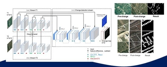
Step 1: Pairwise VHR images are clipped according to the corresponding size, and then the whole Images T1 and T2 of pairwise H × W × C are put into the network.
Step 2: The training is carried out on the training set or verification set by the DSMS-FCN network joining ECA. The deep features and deep difference features of paired images were extracted from the same feature space of Stream T1 and Stream T2, and then change detection stream was used to discriminate the changed regions. The relatively rough change probability image U is obtained.
Step 3: CVA is used to calculate the differential image of pairwise VHR images.
Step 4: The change probability image U and the difference image are taken as the input of CRF-RNN unit, and the network weight obtained in step 2 is taken as the initial value, which conduct joint training with pairwise potential CRF-RNN on the training set or verification set. The number of iterations T in CRF-RNN is generally set to 5. Finally, the optimal network weight of PPNet can be obtained.
Step 5: By inputting pairwise test images, the end-to-end network infers the change map of H × W and obtains the changed regions and the unchanged regions.
Output:
1. Change map.
Table 2. Evaluation of the results generated by the different algorithms on Szada-1 of ACD dataset.
MethodPre.Rec.F1OA
RL0.4310.5070.466NA
TBSRL0.4440.6190.517NA
DSCN0.4120.5740.479NA
CXM0.3650.5840.449NA
SCCN0.2240.3470.287NA
STANet0.4550.6350.530NA
FC-EF0.47290.43990.45580.9341
FC-Siam-Conc0.45620.48080.46820.9395
FC-Siam-Diff0.60530.45610.52020.9349
DSMS-FCN0.60760.48330.56160.9430
DSMS-FCN-FCCRF0.56840.51860.54230.9440
DSMS-FCN-ECA(Ours)0.66400.50230.57190.9420
PPNet(Ours)0.67360.48190.56190.9485
Table 3. Evaluation of the results generated by the different algorithms on LEVIR-CD dataset.
MethodPre.Rec.F1OAKappa
FC-EF0.83980.67230.74680.97680.7348
FC-Siam-Conc0.93070.75590.83420.98470.8263
FC-Siam-Diff0.93530.73740.82470.98400.8164
DSMS-FCN0.93590.73420.82290.98390.8146
DSMS-FCN-FCCRF0.93600.73440.82300.98390.8147
DSMS-FCN-ECA(Ours)0.92770.77300.84330.98540.8357
PPNet(Ours)0.91930.79190.85080.98590.8435
Table 4. Ablation study of FCCRF algorithm, CRF-RNN unit and ECA unit on the LEVIR-CD test set.
MethodFCCRFCRF-RNNECAF1OAKappa
DSMS-FCN(base)0.83540.98490.8276
DSMS-FCN-FCCRF0.83540.98490.8276
DSMS-FCN-CRF-RNN0.83990.98520.8324
DSMS-FCN-ECA0.84330.98540.8357
PPNet0.85080.98590.8435
Table 5. Comparative study of SE attention and ECA based on DSMS-FCN net.
MethodF1OAKappa
DSMS-FCN-SE0.84000.98520.8324
DSMS-FCN-ECA0.84330.98540.8357
Publisher’s Note: MDPI stays neutral with regard to jurisdictional claims in published maps and institutional affiliations.

