Article

InSAR Modeling and Deformation Prediction for Salt Solution Mining Using a Novel CT-PIM Function

1
Laboratory of Radar Remote Sensing Applications, Changsha University of Science & Technology, Changsha 410114, China
2
Hunan Key Laboratory of Remote Sensing of Ecological Environment in Dongting Lake Area, Changsha 410114, China
3
School of Traffic and Transportation Engineering, Changsha University of Science & Technology, Changsha 410114, China
4
School of Electrical and Information Engineering, Changsha University of Science & Technology, Changsha 410114, China
5
School of Geosciences and Info-Physics, Central South University, Changsha 410083, China
*
Author to whom correspondence should be addressed.
Remote Sens. 2022, 14(4), 842; https://doi.org/10.3390/rs14040842
Submission received: 7 January 2022 / Revised: 6 February 2022 / Accepted: 8 February 2022 / Published: 10 February 2022

Abstract

:
Deformation prediction for a salt solution mining area is essential to mining environmental protection. The combination of Synthetic Aperture Radar Interferometry (InSAR) technique with Probability Integral Method (PIM) has proven to be powerful in predicting mining-induced subsidence. However, traditional mathematical empirical models (such as linear model or linear model combined with periodical function) are mostly used in InSAR approaches, ignoring the underground mining mechanisms, which may limit the accuracy of the retrieved deformations. Inaccurate InSAR deformations will transmit an unavoidable error to the estimated PIM parameters and the forward predicted subsidence, which may induce more significant errors. Besides, theoretical contradictory and non-consistency between InSAR deformation model and future prediction model is another limitation. This paper introduces the Coordinate-Time (CT) function into InSAR deformation modeling. A novel time-series InSAR model (namely, CT-PIM) is proposed as a substitute for traditional InSAR mathematical empirical models and directly applied for future dynamic prediction. The unknown CT-PIM parameters can be estimated directly via InSAR phase observations, which can avoid the error propagation from the InSAR-generated deformations. The new approach has been tested by both simulated and real data experiments over a salt mine in China. The root mean square error (RMSE) is determined as ±10.9 mm, with an improvement of 37.2% compared to traditional static PIM prediction method. The new approach provides a more robust tool for the forecasting of mining-induced hazards in salt solution mining areas, as well as a reference for ensuring the environment protection and safety management.

Graphical Abstract

1. Introduction

By the end of 2018, the reserves of mirabilite deposits in China had reached up to 117.297 billion tons [1]. For mirabilite production in the salt mining deposits, water-soluble exploitation, with comprehensively multi-propulsion through groups of drilling wells, is the primary mining mode in salt solution mining area. Attributing to the multi-direction of water-soluble mining activities, the upper layer of the rock salt cavern is prone to overburden, or even serious collapse [2]. As long as the roof of the cavern uplifts to the ground surface, a large pit, which may cause potential damage to the nearby infrastructures, will be formed [3]. In addition, accumulated water-soluble mining activities may cause significant lithological changes of the underground rock, even inducing a serious pumping of brine and water salinization. Therefore, long-term spatio-temporal deformation prediction of salt solution mines are of considerable importance to the environmental protection and safety management. The multi-temporal interferometric synthetic aperture radar (MT-InSAR) is an advanced space-to-earth observation technology developed in recent years. Compared with traditional InSAR technology, MT-InSAR technology has been reported to be more effective and applicable for deriving ground deformations (i.e., mining area or infrastructures) [4,5,6,7,8,9,10,11,12,13]. However, the single MT-InSAR has a limitation in that it can only obtain the deformation sequences during SAR acquisition dates; the subsequent future displacement beyond the span of the SAR observations cannot be acquired. To compensate for the limitation, researchers have incorporated InSAR deformation observations into the Probability Integral Method (PIM), which has successfully solved the problems, such as surface deformation space calculation and overlying strata movement prediction [14,15,16,17,18,19,20,21,22]. The basic idea for those studies is firstly using the traditional MT-InSAR technique to generate the line-of-sight (LOS) deformation results as input dataset to estimate the PIM parameters; then, the corresponding subsidence sequences for the future period can be predicted based on the PIM prediction model. Those researchers have successfully retrieved the spatio-temporal deformation characteristics and achieved the forward prediction of mining-induced deformations, which proves that the combination with PIM theory is an efficient and feasible complementation to single MT-InSAR technique.
However, there still exist limitations: Firstly, according to previous studies, pure empirical mathematical models (i.e., linear model or linear model combined with periodical function) are mostly utilized to generate the InSAR observations, and the underground mining subsidence mechanism is not considered in the InSAR modeling procedure. In MT-InSAR data processing, the deformation modeling procedure determines the temporal functional relationship between the interferometric phase observations and the parameters. The evolution of mining-induced surface displacement is a complex physical non-linear process, varying with time. Apparently, modeling a physical process with a single empirical mathematical function cannot accurately describe the underground deformation mechanisms and, thus, may have a great impact on the accuracy of the generated InSAR deformation observations. Secondly, inaccurate InSAR deformation results will transmit an unavoidable error to the estimated PIM parameters, then, secondly, propagating to the future subsidence prediction, leading even larger errors in the predicted displacements. Finally, the traditional mathematical models (i.e., linear model or linear model combined with periodical function) used in the deformation monitoring is not consistent with the PIM used in the future deformation prediction, which is based on random medium theory. Using InSAR deformation observations generated via a simple linear model to estimate parameters for a complex non-linear model may not be reasonable. Consequently, contradiction and inconsistency between the InSAR deformation model and the future prediction model is the third limitation.
Based on the above analysis, in order to improve the accuracy of deformation prediction, we propose a novel InSAR deformation model, which can better describe the dynamic evolution disciplines of the underground mining subsidence in the MT-InSAR deformation modeling procedure, as well as be directly used to the forward deformation prediction. The novel model is based on the Coordinate-Time (CT) function (namely CT-PIM) and used as a substitute for traditional InSAR models. CT-PIM improves the static PIM via integrating the temporal parameter to achieve the description of the temporal dynamical characteristics of the mining-induced subsidence. Considering the physical subsurface mechanism, CT-PIM can describe the temporal dynamical characteristics of the mining-induced subsidence more realistically. The PIM parameters are introduced into InSAR time-series phase functions and can be estimated via the phase observations, which can avoid the secondary error propagation from the inaccurate InSAR deformations to the subsequent deformation prediction. Subsidence can be predicted directly based on CT-PIM, which implements in opposition to the deficiency of inconsistency and lack of reasonability between the InSAR model and the forward prediction model. Consequently, the new method is expected not only to enrich the time series InSAR modeling theory but also provide a more robust tool for forecasting mining-induced hazards in mining areas.

2. Materials and Methods

The CT-PIM, including the Coordinate-Time function, and the PIM parameters are introduced in Section 2.1. The InSAR modeling based on CT-PIM is derived in Section 2.2, together with the final functional relationship between the time series phase observations and the PIM parameters.

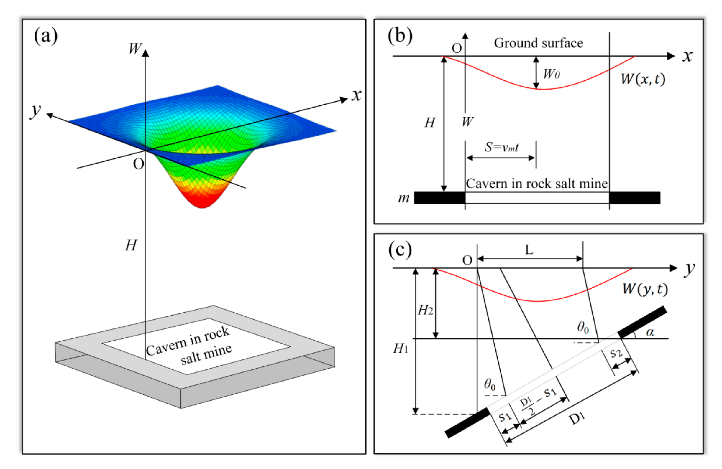
2.1. Dynamic Coordinate-Time Probability Integration Model

The Coordinate-Time (CT) function was proposed in Reference [23], which improved the traditional static PIM with introducing the temporal parameter t , thus being referred as CT-PIM hereinafter. It has proven to be effective and reliable in the application for the dynamic ground deformation prediction caused by mining activities. The surface subsidence described in CT-PIM function is as follows [23]:
W   ( x ,   y ,   t ) = 1 w 0 W   ( x ,   t ) W   ( y ,   t ) ,
where ( x ,   y ) denotes the coordinate of the surface point, and W   ( x ,   y ,   t ) is the surface vertical subsidence related to mining activities at time t ; w 0 is the maximum settlement, which can be written as w 0 = m q · c o s α , where m is the thickness of the mine, q is the subsidence factor, and α is the dip angle of the layer. W   ( x ,   t ) and W   ( y ,   t ) can be expressed as follows:
(1)
When the dip direction of the working face is under critical extraction, whereas the strike is under subcritical extraction. This happens in the practical condition that the advancing distance is longer than the depth along the dip direction. The ground subsidence can be written as (the schematic diagram is shown as Figure 1b) [23]:
W x , t   = w x 2 e r f π + e r f π v m t n H r r x n H w x 2 e r f π + e r f π v m t r x + H a + b x H a + b x 3 r n H <   x   < 1.3 r w 0 2 e r f π r + e r f π v m t + H / t a n ω 2 x r 1.3 r x ,
where w ( x ) can be calculated based on the principles of static PIM following the equation: w ( x ) = w 0 2 e r f π x r + 1 ; e r f is a probability integral function: e r f ( π r x ) = 2 π 0 π r x e u 2 du (where u is the integral parameter, r is the main influence radius, r = H t a n β ; H is the mining depth and t a n β is the tangent of the main influence angle); n H is the starting distance, describing the advancing distance of the working face when the ground point starts to move; n is the starting factor; ω is the static leading influence angle (in degrees); v m is the mining advancing speed; and the coefficients a and b can be expressed as a = 117 r ω n H 1.3 r n H and b = ω 90 1.3 r n H , respectively.
(2)
When the strike direction of working face is under critical extraction, whereas the dip is under subcritical extraction. This happens in the most practical condition of the coal mining activities, since the strike direction is better to contain a longer advancing distance (even up to several kilometers, much deeper than the depth along the strike), which can easily satisfy the critical extraction condition. The surface subsidence can be written as (the schematic diagram is shown as Figure 1c) [16]:
W   ( y ,   t ) = w 0 2 e r f π y r 1 e r f π y L r 2 ,
where y denotes the vertical coordinate of the ground point in the mining area; r 1 and r 2 represent the main influence radius along the down-dip, and up-dip directions, respectively, which can be expressed as r 1 = H 1 t a n β 1 and r 2 = H 2 t a n β 2 . H 1 and H 2 are the mining depths along the down-dip, and up-dip directions, respectively. Here, H 1 = H D 1 2 s i n α and H 2 = H + D 1 2 s i n α ; L is the estimated length of strike working face, which can be expressed as L = D 1 s 1 s 2 s i n θ 0 α s i n θ 0 ; D 1 is the inclined length of working face; s 1 and s 2 are the offsets of inflection point along down-dip and up-dip directions of the working panel; θ 0 is the mining influence angle, which can be calculated following θ 0 = 90 ° k α .
It is worth noting that, when the strike of the working face is under subcritical extraction, the final deformation should be estimated via multiplying a coefficient: C x m = W x m W 0 < 1 , where W 0 = m q · c o s θ . W x m is the maximum value of W   ( x ,   t ) , which can be calculated according to the first equation in Equation (2), under the assumption that the tendency has reached an extreme exploitation [16]. Similarly, when the dip of the working face is under subcritical extraction, then a dip mining degree coefficient, C y m = W y m W 0 < 1 , should be multiplied with it, where W y m denotes the maximum value of W   ( y ,   t ) in Equation (3).

2.2. InSAR Modeling Based on CT-PIM (InSAR-CTPIM)

For each high coherence pixel in the i -th interferogram [24,25,26], its corresponding interferometric phase can be expressed as:
δ φ i = δ φ d e f i + δ φ t o p o i + δ φ o r b i t i + δ φ a t m i + δ φ n o i s e i + Δ φ n o n i 4 π λ Δ d i + 4 π B i λ R s i n θ Δ H i + Δ φ r e s i ,
where λ is the radar wavelength; Δ d is the LOS accumulated deformation spanning the time period of the i -th interferogram, referred as the low-pass (LP) component hereinafter; Δ φ t o p o i represents the residual topographic phase component; Δ φ t o p o i = 4 π B i λ R s i n θ Δ H i , where B i defines the perpendicular baseline, θ the incident angle, R the sensor-target distance, and Δ H the residual elevation, which is an unknown parameter; Δ φ r e s i denotes the final residual phase, which includes the phase noise, atmospheric delay, and the high-pass (HP) deformation component [27].
During the extraction of the brine from the wellhead, the deformation of the surface caused by the change of the top pressure in the cavern is dominantly along the vertical direction. Besides, the upper dissolution rate of the drilling solution mining process is approximately twice of the side dissolution rate [28]. Therefore, compared with the vertical subsidence, the horizontal displacement caused by water-soluble mining is relatively minor, and omitted hereinafter. Then, the functional relationship between the LOS deformation and the ground subsidence can be expressed as:
Δ d i = d L O S t B i d LOS t A i = W   x ,   y ,   t B W   x ,   y ,   t A · c o s θ ,
where W   ( x ,   y ,   t B ) and W   ( x ,   y ,   t A ) are the corresponding dynamic subsidence at t B and t A , respectively. Substituting Equation (5) into (4), the functional relationship between the InSAR phases and PIM parameters can be written as:
δ φ i = 4 π λ W   x ,   y ,   t B W   x ,   y ,   t A · c o s θ + 4 π B i λ R s i n θ Δ H i + Δ φ r e s i ,
where the geological parameter G P = [ m ,   α ,   H ,   D 1 ,   ω ] of the rock salt mine can be determined according to the in-situ investigation of the study area or the materials provided by the mining company, which can be regarded as known parameters. The unknown parameters to be solved here are U P = [ q , t a n β ,   s 1 ,   s 2 ,   k ,   n ] . Among them, q is within the range of [0.01, 1], t a n β , t a n β 1 , and t a n β 2 are all distributed within the range of [1, 3.8], and both s 1 and s 2 are within the range of [0.05H, 0.3H]. The propagation influence angle of mining is θ 0 = 90 ° k α . Here, k ranges from 0.5 to 0.8, and the starting distance coefficient n ranges from 1/7 to 1/2 [14,16,23]. Equation (6) describes the temporal functional relationship between the InSAR time series phases and the PIM parameters, which is referred as InSAR-CTPIM, and will be applied for the time series deformation generation.

2.3. CT-PIM Parameters Estimation Based on InSAR Phases

If N + 1 scenes covering the whole study area are acquired at dates ( t 0 ,   t 1 ,   ,   t N ) , then M differential interferometric pairs are generated accordingly. For each pixel ( x ,   y ) on the differential interferograms, M InSAR functions (in Equation (6)) based on the phase observations can be established. If M is higher than six, the unknown parameters U P = [ q , t a n β ,   s 1 ,   s 2 ,   k ,   n ] can be estimated. The ill-conditioned nature of the phase functions (introduced as Equation (6)) has also been tested to ensure the robustness. For each pixel ( x ,   y ) on the differential interferograms, M InSAR functions based on the phase observations can be established. The condition number C o n d ( A ) = A A 1 is estimated as 18 here, where A defined the coefficient matrix of the phase functions. The value of C o n d ( A ) implies that no ill-conditioned phenomenon exists in the functions.
The solving of Equation (6) is obviously a non-linear parameter estimation problem. The Genetic Algorithm (GA), combined with the Simplex Method (SM), is introduced here to estimate UP. GA processes the advantages of global optimization searching ability and unrestricting to different model forms [29], and it has been proven to be feasible in solving the problems of non-linear parameter estimation [30]. It generates the optimized estimations in form of population individuals following the principle of fitness function minimization [31]. However, the disadvantages of slow convergence speed and low accuracy are also prominent for GA. SM has proven to be an efficient tool in solving the non-linear estimation problems when combined with GA, which can refine the GA generated results effectively [32]. Consequently, the combination of GA and SM, namely GASM, is adopted here to effectively estimate the unknown parameters.
As for Equation (6), each individual gene is U P = [ q , t a n β ,   s 1 ,   s 2 ,   k ,   n ] , and the fitness function here is:
f = Δ φ r e s i = m i n ,
where Δ φ r e s i denotes the residual phase in Equation (6). After the iteration of population selection, crossing over, and evolution for each individual gene until the minimum fitness function value condition is satisfied, the final obtained individual genes, which are treated as the initial GA-solutions for PIM parameters, will be taken as the input initial values of SM. Then, SM is utilized to improve the accuracy of GA estimations after the global searching, and the corresponding SM-output results are determined as the final solutions for PIM parameters [33].

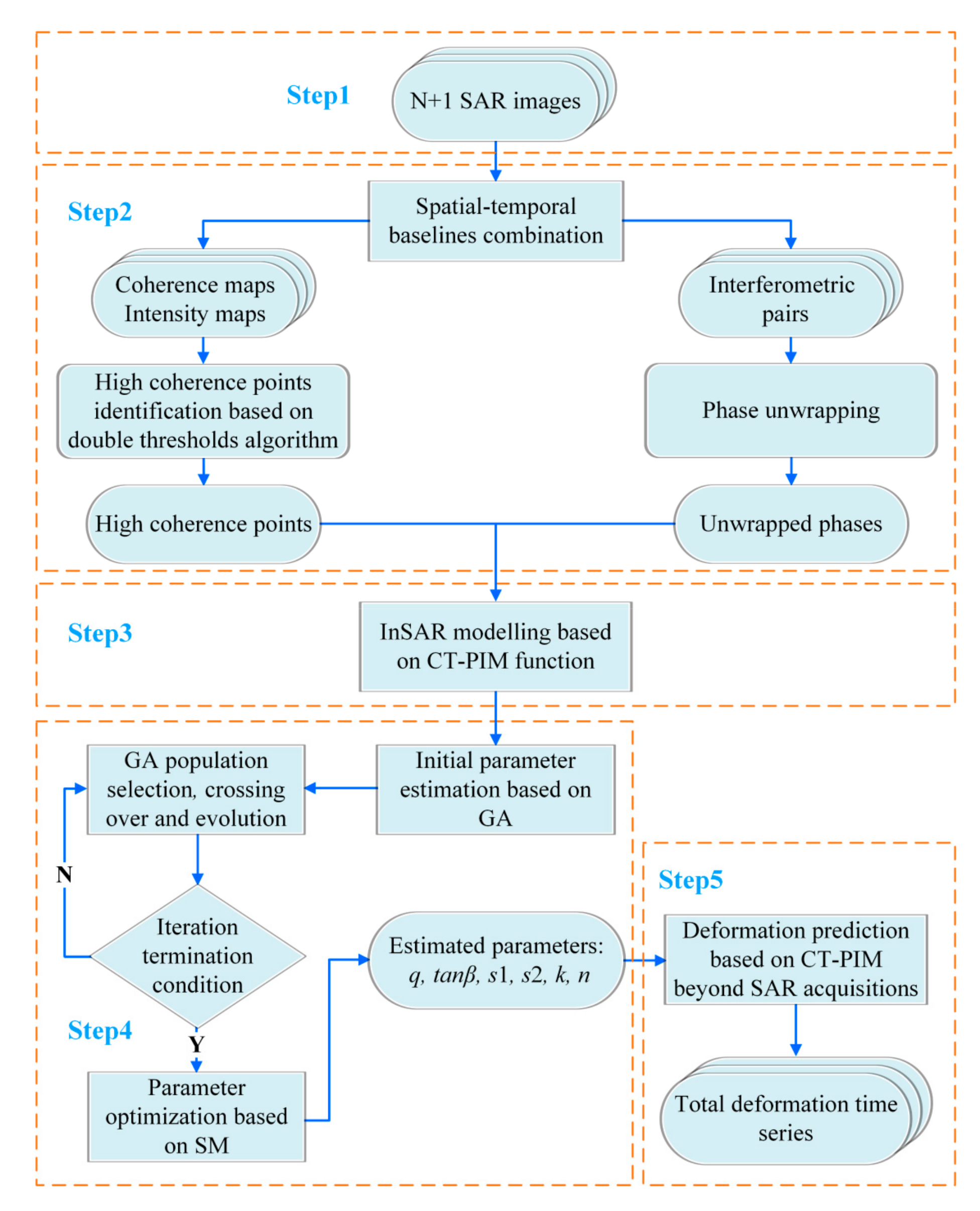
2.4. Flow Chart and Processing Steps

Figure 2 displays the processing flow of deformation prediction using the CT-PIM function. The steps are as follows:
  • Differential Interferometry according to the N + 1 SAR images covering the study area.
  • High-coherent candidates extraction considering both the average coherence and the amplitude dispersion index.
  • InSAR modeling following the CT-PIM function, which establishes the functional relationship between InSAR phases and unknown PIM parameters.
  • PIM parameter estimation based on Genetic Algorithm and Simplex Method (GASM) [32,33], which includes GA global searching to generate the initial values of PIM parameters and SM to optimize the GA solutions.
  • Forward dynamic subsidence prediction beyond the spans of SAR acquisitions based on CT-PIM function introduced as Equation (1).

3. Results

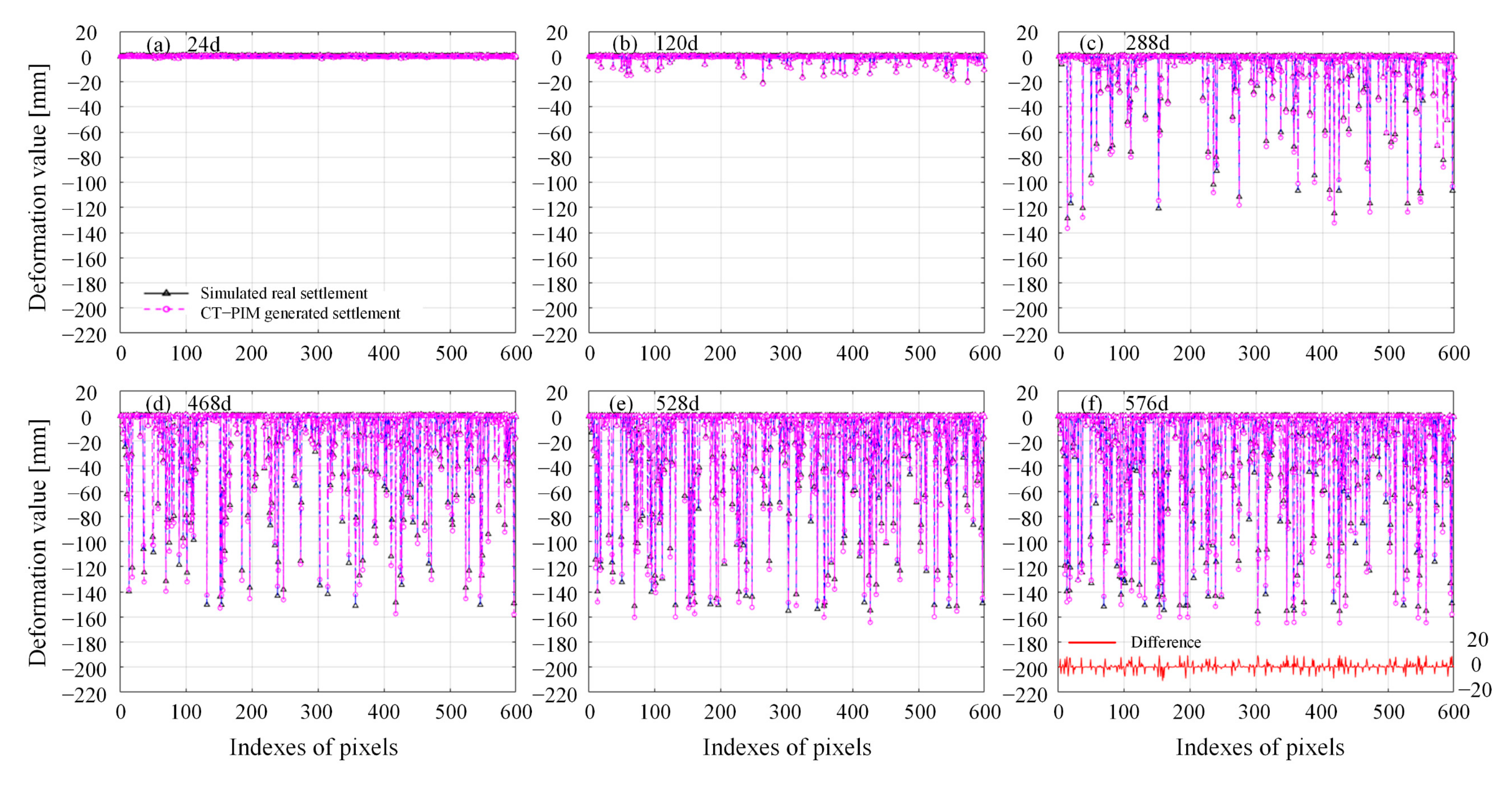
3.1. Simulated Experiment

A simulated experiment was designed and executed to evaluate the feasibility and accuracy of the proposed method. Satellite parameters used in the simulated experiment were set according to Sentinel-1 A spaceborne parameters, which was to keep consistent with the real data experiment. The geological parameters m , α , H , D 1 , ω of the strata overlying the saline layer were set as 0.66 m, 4.5°, 600 m, 300 m, 80° according to real data collected by the company in charge of the mining activity in the area. The advancing speed v m at the simulated experiment was set as 0.24 m/d, which was also according to the real data (will be discussed in Section 3.2.1). The simulated true values of U P were set primarily as 0.504, 1.560, 30.310 m, 16.080 m, 0.524, 0.167.
After setting those parameters, the time series settlement field could be generated according to Equation (1), which would be used as the real settlement field compared with the subsidence generated based on the InSAR-CTPIM processing. The selected images of the simulated real settlement field are shown in Figure 3. InSAR phase functions can be simulated according to Equation (6), and the residual elevation Δ H was simulated via Gaussian random simulator with its magnitude within [−20, 20] m. The random noise with a variance from 0 rad to 0.65 rad was added in the simulation. The random noise we added here can be expressed as N o i = s q r t   ( 0.65 )     r a n d n   ( 60 ,   60 ) , where Noi represents the noise; s q r t   ( 0.65 ) represents the variance of 0.65 rad; r a n d n is the random noise function in MATLAB; and ( 60 , 60 ) is total simulated size of the phase function. Totally, 600 indexes of pixels were randomly extracted for the subsequent quantitative comparison with the CT-PIM generated deformation. In order to evaluate the impacts of different numbers of interferometric pairs on the corresponding generated deformation results, the simulation experiments with a multi-master connection were designed [34]. Six subgroups of simulation were carried out, with the number of interferometric pairs as 10, 15, 20, 25, 30, and 35, respectively, which also represented the number of InSAR phase functions. The corresponding GASM procedure was performed to obtain the CT-PIM parameters based on the simulated InSAR phase observations, and the final estimated subsidence could be obtained via Equation (1). The parameters, such as the spatio-temporal baselines, used in the simulation were set according to the real data experiment (in Section 3.2.2).
To estimate the unknown parameters of CT-PIM, the maximum iteration number, the population size, the crossover probability, and the mutation probability in GASM algorithm were set as 400, 60, 0.5, and 0.2, empirically. After the SM secondary optimization, the final optimal estimations of the CT-PIM parameters could be generated for each subgroup of simulation. Substituting the obtained parameters into Equation (1), the time series settlement field could be generated.
Figure 4 illustrates the relative errors for each parameter between the CT-PIM generated values and the simulated real ones under a different number of interferometric pairs. The lower the relative error is, the higher is accuracy suggested for the CT-PIM estimated parameter. As can be seen from the figure, generally, the relative errors decrease with the increase of interferometric numbers. Under a multi-master connection, a stack of 20 interferograms is acceptable in our cases. It can also be noted from Figure 4 that, among the six parameters, q and t a n β were more sensitive with higher curvature slopes than the remaining four parameters.
We extracted the interferometric pairs of 10 and 35, respectively, to show a quantitively comparison with the simulated real values (shown as Table 1 and Table 2). The results show that the use of 35 interferometric pairs under the multi-master connection to estimate the unknown parameters is evidently more accurate (for instance, the relative error for q is only 4.8% under 35 pairs compared with that of 10.4%). Therefore, we finally determined to use 35 interferometric pairs (noise level with a variance of 0.65 rad) under the multi-master connection in the real data experiment. It can also be noted that, among the six parameters, the relative error of s 1 is relatively large, both in Table 1 and Table 2, with 8.6 % and 6.2%, respectively. This is consistent with the results of the sensitivity analysis in Section 3.3.3.
Figure 5 shows the comparison results between the selected time series settlement generated by CT-PIM and the simulated settlement with 600 pixels (35 interferometric pairs, multi-master connection, with a noise variance level of 0.65 rad), and the differences are illustrated in Figure 5f in red polylines. It can be noted that the two groups of results demonstrate good agreement even under a relatively high noise level of 0.65 rad, and the max deviation increases with the time span. According to the quantitative statistics for Figure 5a–f, the number of points with the deviations within [−5, 5] mm account for 100%, 100%, 97%, 90%, 87.6%, and 85.8% of the total number of points for spans of 24 days, 120 days, 288 days, 468 days, 528 days, and 576 days, respectively, and the corresponding maximum deviation is 0.1 mm, 1.3 mm, 7.9 mm, 9.3 mm, 9.5 mm, and 9.6 mm, respectively. Compared with the maximum subsidence for each period (i.e., 165 mm at 576 days), the deviation was relatively minor (a 9.6 mm deviation occupy only 5.8% approximately). To quantitatively evaluate the distribution of the deviations, statistical analysis for the probability distribution was carried out. Figure 6 demonstrates the probability distribution of the average deformation deviations with 600 pixels. As determined, the magnitudes of errors are concentrated within a relatively low ranges, with 83.8% of points distributed within [−2, 2] mm and all the pixels distributed within [−6, 6] mm, which implies that the proposed method is of promising accuracy. The RMSE between the CT-PIM generated value and the simulated real settlement is estimated as ±4.5 mm.

3.2. Real Data Experiment

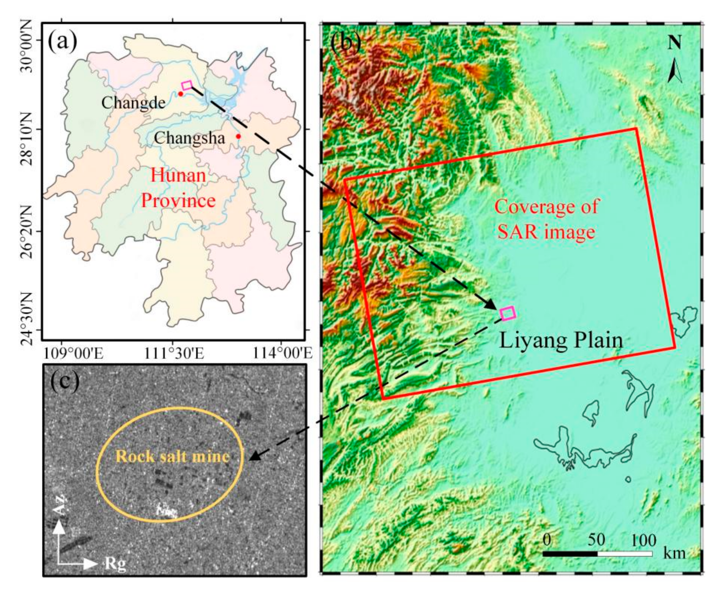
3.2.1. Study Area and SAR dataset

A salt mine, located in China, was selected as the study area. Figure 7 displays the location of our test area in Hunan Province and the corresponding coverage of SAR satellite images. The red rectangle in Figure 7b represents the spatial coverage of Sentinel-1 A image obtained by a satellite ascending geometry, and the purple rectangle represents the area of interest. The mine is located in the central part of Liyang Plain, with the characteristics of abundant natural water systems, numerous large and densely distributed ponds, crisscrossing artificial channels, and extensive surface paddy fields. Long-term drilling soluble mining activities have caused serious land salinization, which imposed significant influences to the surrounding environment (see Figure 8a). The mining-induced accumulated subsidence also led to cracks on the ground surface of roads, which imposed potential damage to infrastructures built on the nearby residential area (see Figure 8b,c). Gradually accumulated ground subsidence may also generate an obvious stagnant water pit (shown as Figure 8d, with a settlement approximately of 1.5 m).
Figure 9 shows the local geological asset. The underground stratums mainly include Lower Tertiary and Quaternary. The lithological components over this area mainly consist of mudstone, dolomite, siltstone, gypsum, mirabilite, and glauberite. Anhydrous Glauber salt ( Na 2 SO 4 , 62.76–78.8%) produced in this area exist in the salt-bearing section ( E 2 x 3 ) of Neogene Formation. Argillaceous dolomitic mirabilite is the dominate lithological component, which distributes over the up layer, bottom layer, and interlayer and belongs to weak layered rock mass. The poor stability of the rocks in this area makes the ground surface vulnerable to soften and collapse.
According to the above lithological characteristics of the upper layer on the working surface and the collected geological materials of the mine, the aforementioned lithologic geological parameters GP (see Table 3) is set as GP = [3 m, 5.7°, 240 m, 258 m, 80°] according to the geological materials provided by the mining company. The advancing speed v m is practically calculated according to properties of the sedimentation funnel in the mining area, which follows the equation v m = S t = 0.056 m/day, where S denotes the mean radius for the sedimentation funnels, and t denotes the time span of the mining activities.

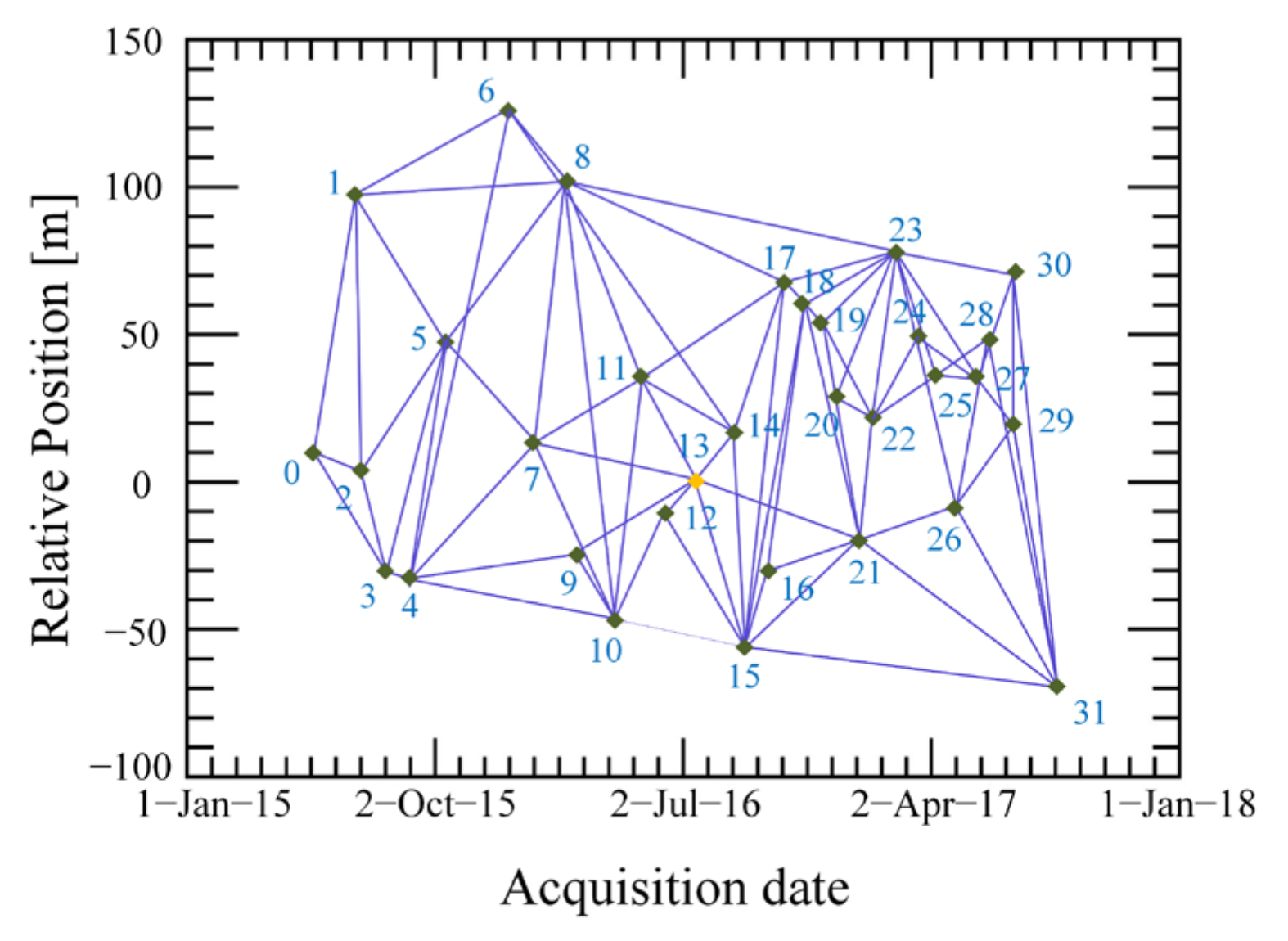
3.2.2. SAR Data Acquisition and Preprocessing

A total of 32 Sentinel-1A scenes with ascending geometry spanning the period from 15 June 2015 to 15 August 2017 were collected for the differential interferometric dataset processing. The unwrapped interferometric pairs with small spatial-temporal baselines were generated via SARScape 5.2 and ENVI 5.3. The SAR sensor parameters and spatial -temporal baselines are shown in Table 4 and Figure 10, and the subsequent high coherence points extraction, InSAR deformation modeling, CT-PIM parameter estimation, and deformation generation were all executed via MATLAB software. In the preprocessing of differential interferometry, the multi-look ratio of SAR image was set as 5:1, with the sampling resolutions as 9.022 m along azimuth, and 7.368 m along range direction, respectively. Spatial-temporal interferometric baselines were set lower than 150 m and 420 days, respectively, with all the images registered and resampled to a super master image (acquired at 3 July 2016). External 30 m resolution Shuttle Radar Topography Mission Digital Elevation Model (SRTM DEM) data was used to filter the terrain phase [35]. The procedure of phase unwrapping was executed with the Minimum Cost Flow (MCF) method. After artificially eliminating the unsatisfied interferometric pairs with poor unwrapping effect, totally, 58 unwrapped differential interferograms were generated [36,37]. Thresholds for moderate to high coherent points were set as 0.45 for coherence, and 0.35 for mean amplitude dispersion index. Finally, a total of 6027 candidates in the mining area were extracted.

3.2.3. PIM Parameter Estimation Based on InSAR-CTPIM

Before the novel InSAR-CTPIM processing being applied for the study area, the traditional SBAS-InSAR with multi-linear velocity model was performed to capture the spatial-temporal deformation characteristics over the rock salt mine. As shown in Figure 11, it can also be determined that apparent multi subsidence bowls developed during the observations from a spatial view. This phenomenon is related to drilling water-soluble mining activities. As in situ investigated, the mining mode for the test rock salt mine is multi-well groups connectivity, where more than two wells are connected for each well group during the drilling soluble mining; thus, multi settlement funnels will be formed around each well group. Since the CT-PIM model is based on a single subsidence funnel, it is difficult to accurately cover the whole test area containing complex multi settlement funnels with a single CT-PIM. Consequently, we divided the area into seven sub-settlement funnels, which are shown as Figure 11b, with the subsidence image at 15 August 2017 as the background.
In InSAR-CTPIM processing, 24 images from 15 June 2015 to 11 January 2017 were extracted to estimate the CT-PIM parameters with GASM algorithm, which would be used to generate the corresponding deformation sequences following the step 4 of the procedures introduced in Section 2.4. Based on the obtained CT-PIM parameters, the remaining eight images (from 16 February 2017 to 15 August 2017) were reserved to validate the forward predicted deformation generated by CT-PIM following the step 5. During the GASM procedure, seven sub-funnels were processed separately, with seven groups of parameters generated, which is shown in Table 5.

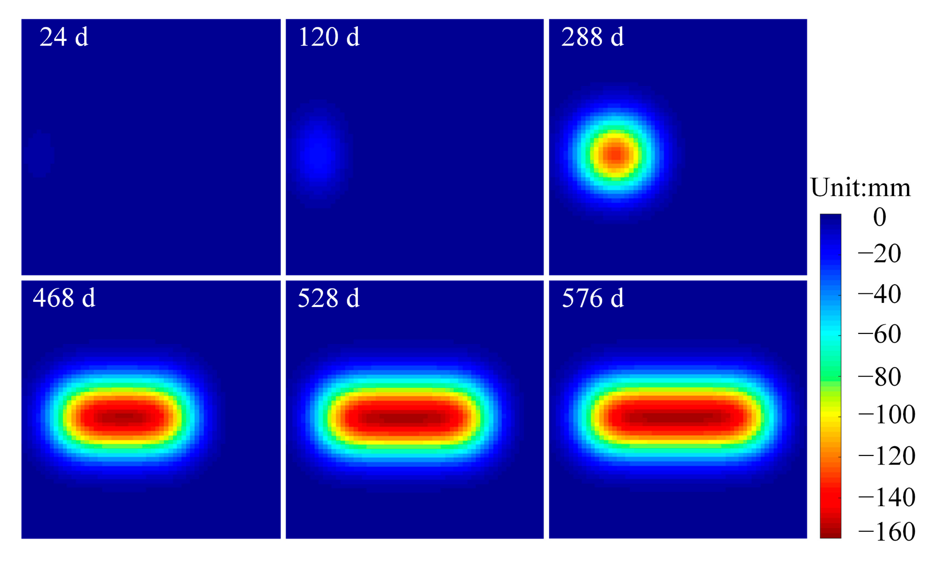
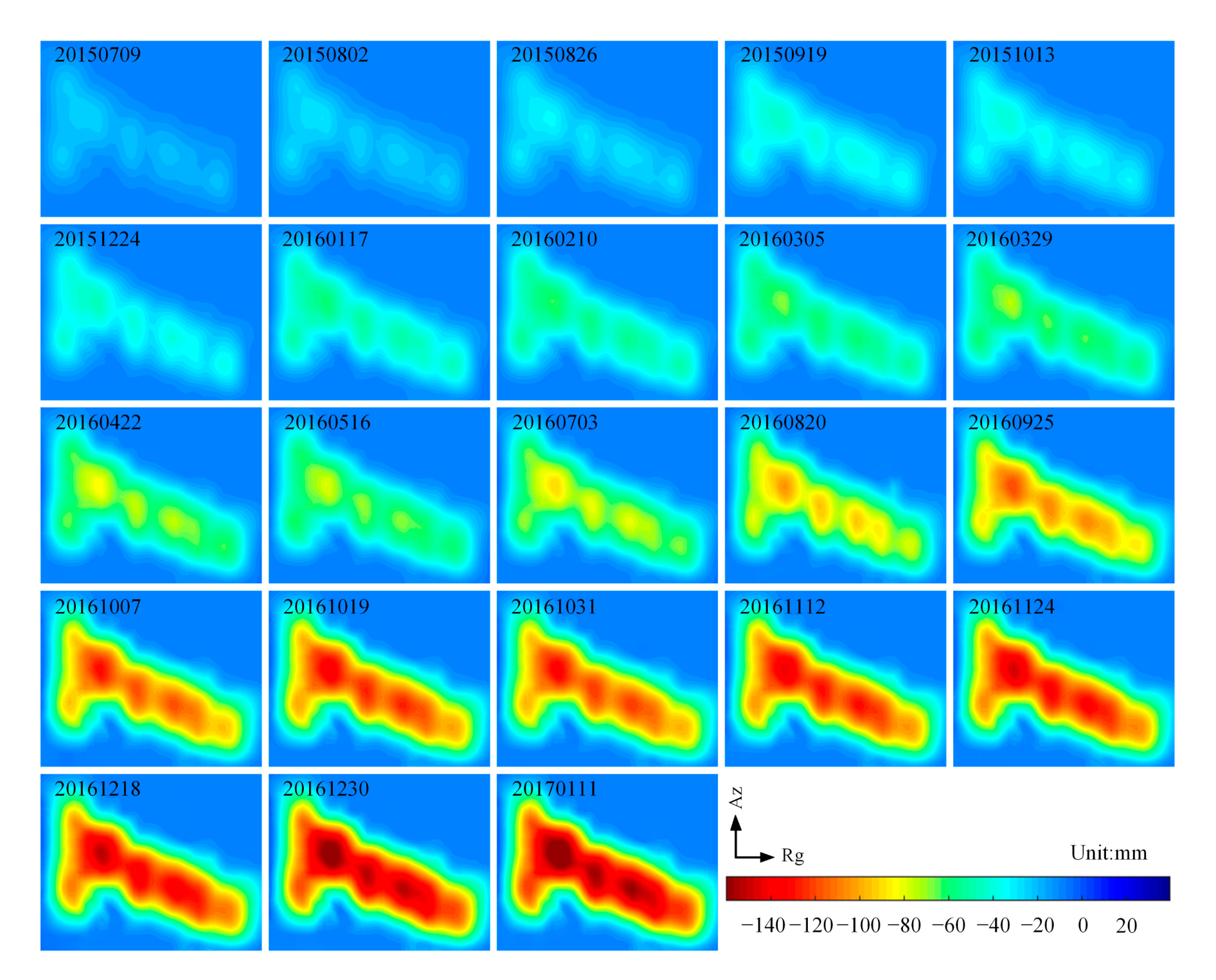
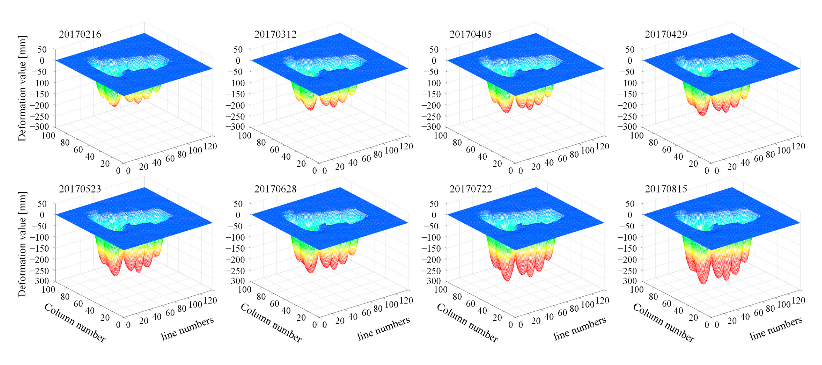
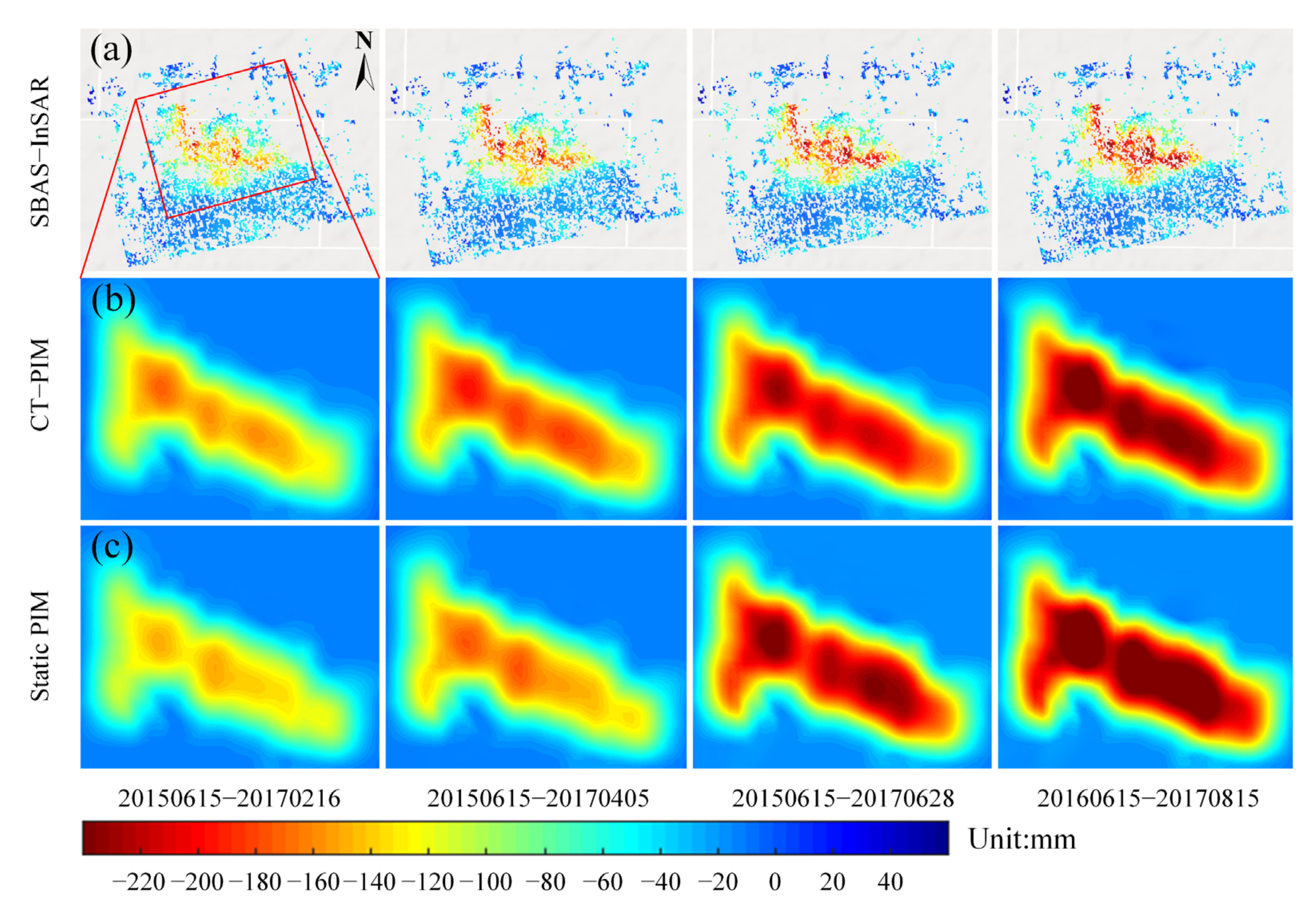
3.2.4. Deformation Prediction Based on CT-PIM

Based on the seven groups of obtained CT-PIM parameters in Table 5, the deformation sequences covered by SAR data acquisition can be derived by InSAR-CTPIM. Figure 12 shows the time series deformation generated spanning from 15 June 2015 to 11 January 2017, which were treated as the deformation monitoring results. The deformation beyond SAR data acquisition can be predicted according to CT-PIM (expressed as Equation (1)). Figure 13 shows the eight 3D scenes (from 16 February 2017 to 15 August 2017) of the predicted subsidence based on CT-PIM, which were treated as the deformation prediction results. From 9 July 2015 to 10 February 2016, the overall deformation of the whole area was relatively stable, with the maximum estimated subsidence as only 52 mm. Obvious subsidence began to occur at 5 March 2016 after an 8-month temporal lag, and the subsiding velocities have increased rapidly since then. Since 20 August 2016, the boundary of the seven sub-settlement bowls has become apparently more distinct, with the maximum subsidence increasing from 110 mm to 205 mm on 11 January 2017. As of 15 August 2017, the maximum subsidence had accumulated up to 294 mm.

3.3. Accuracy Analysis

3.3.1. Accuracy Evaluation for InSAR-CTPIM Monitored Subsidence

The historical leveling measurements from 2 August 2015 to 18 December 2016 for the test mine were collected, which can be used to test the accuracy of the deformation results during the SAR acquisitions obtained by InSAR-CTPIM. The locations of the leveling points (CP1, CP2, …, CP7) are marked in Figure 11a, with the reference point marked as R in the north-east corner. The leveling measurements which covered consistent periods with the SAR acquisition dates were extracted to conduct a more precise comparison with the InSAR-CTPIM monitored subsidence.
Figure 14 shows the comparison between the results of InSAR-CTPIM, SBAS-InSAR, and leveling measurements. The average RMSE of InSAR-CTPIM results was estimated as ±6.9 mm, whereas that of traditional SBAS-InSAR was ±8.5 mm, with an increase of approximately 20.8%. It can be determined that the dynamic settlement obtained by InSAR-CTPIM shows better consistency with the leveling measurements. According to our experiment, almost all the leveling points in the mining area were under a considerable subsiding period. The most serious settlement occurred at CP3, with a value of 156 mm. The RMSE accounts for 4.4% of the maximum settlement, which implies the promising accuracy of InSAR-CTPIM in deriving time series subsidence of the rock salt mine.

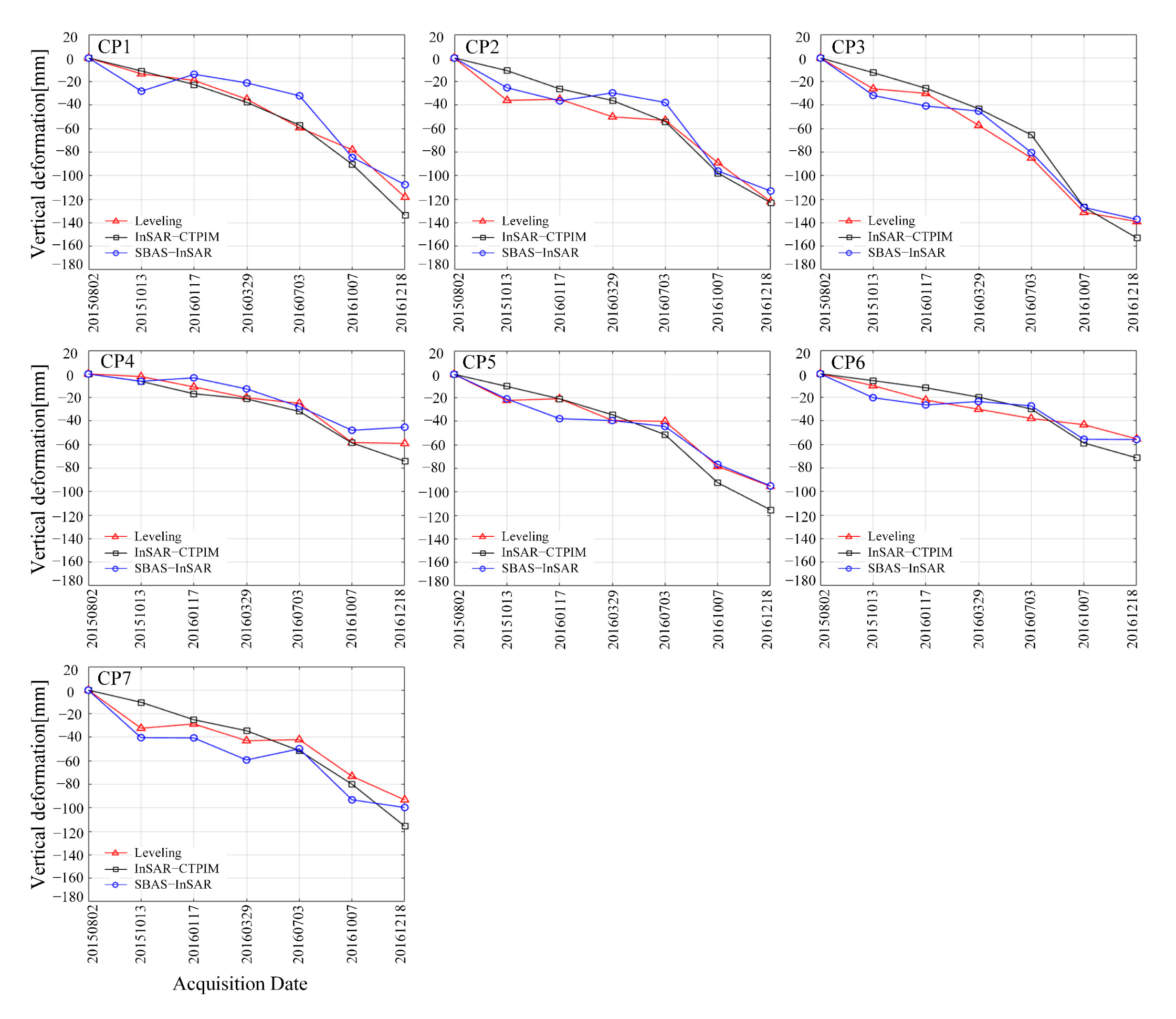
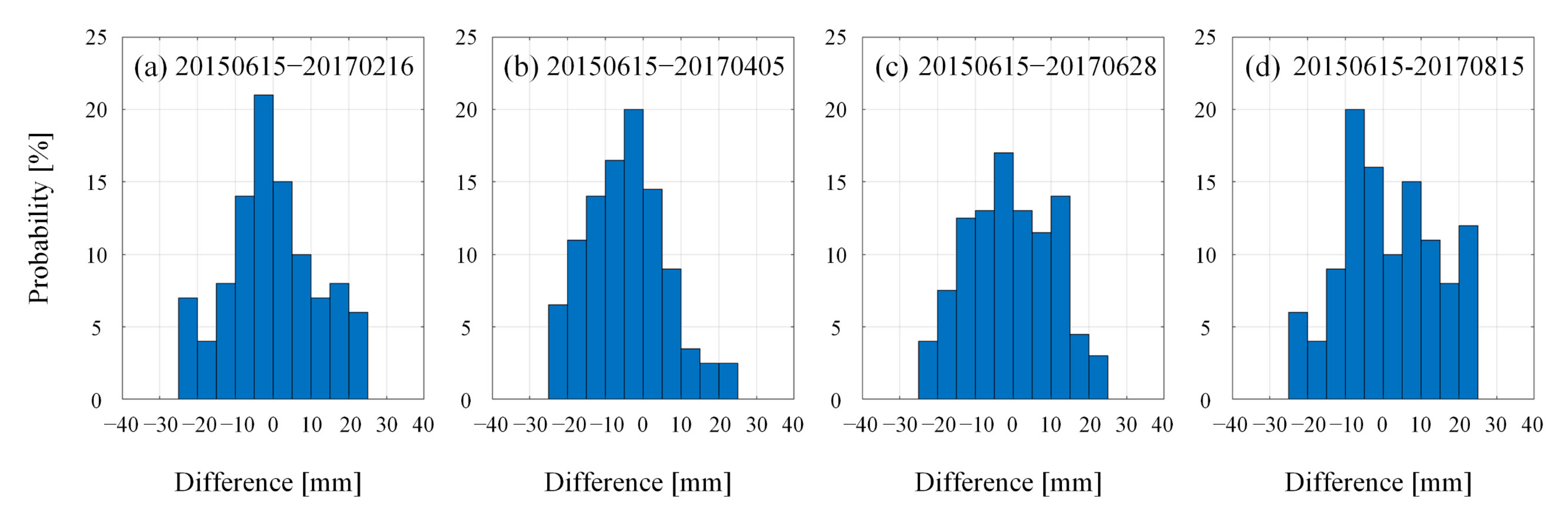
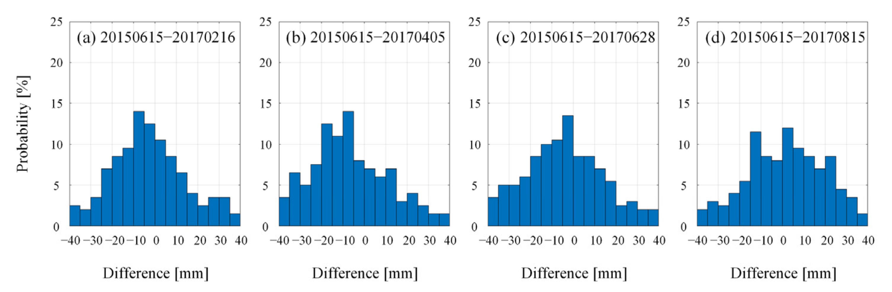
3.3.2. Accuracy Evaluation for CT-PIM Predicted Subsidence

As discussed above, the remaining eight images from 16 February 2017 to 15 August 2017 were reserved to evaluate the forward subsidence prediction results. To compensate for the unavailability of simultaneous periods of leveling measurements, SBAS-derived results were used to be compared with the predicted subsidence. The traditional static PIM prediction method introduced in References [20,38], which inversed the PIM parameters based on a single interferometric pair, was carried out preliminarily to be compared with the CT-PIM predicted results. Four periods of predicted subsidence (spanning from 15 June 2015 to 26 February 2017, 5 April 2017, 28 June 2017, and 15 August 2017, respectively) were extracted, which is shown as Figure 15. The maximum subsidence predicted via static PIM were relatively lower than those of SBAS-InSAR. On 15 August 2017, the maximum subsidence predicted by static PIM was estimated as 325 mm, with a 39-mm difference with the SBAS-derived result, while the difference of CT-PIM is only 8 mm.
For further quantitative analysis, the points located in the subsidence funnels were extracted from Figure 15. The probability distribution was statistically analyzed, and the distribution histograms are shown as Figure 16 and Figure 17. As Figure 16 shows, the residual errors for all the sampled points between CT-PIM predicted subsidence and those of the SBAS results during the four temporal periods are mainly distributed within the range of [−25, 25] mm. The RMSE is estimated as ±12.8 mm, ±12.7 mm, ±12.9 mm, ±13.2 mm, respectively. In contrast, those residual errors for static PIM (shown as Figure 17) are mainly distributed within a more disperse range of [−40, 40] mm, with its RMSE estimated as ±20.2 mm, ±18.5 mm, ±20.7 mm, ±15.8 mm, respectively, which are much higher. Apparently, the distribution of CT-PIM errors is better concentrated than those of static PIM, which indicates a better consistency with the SBAS technique and a higher predictive accuracy. The total STD of those errors for CT-PIM is estimated as ±12.9 mm. It can be inferred that the CT-PIM predicted results show better consistency with the traditional SBAS-derived subsidence than that of static PIM predicted ones, with an increase of 37.2% compared to that of static PIM.

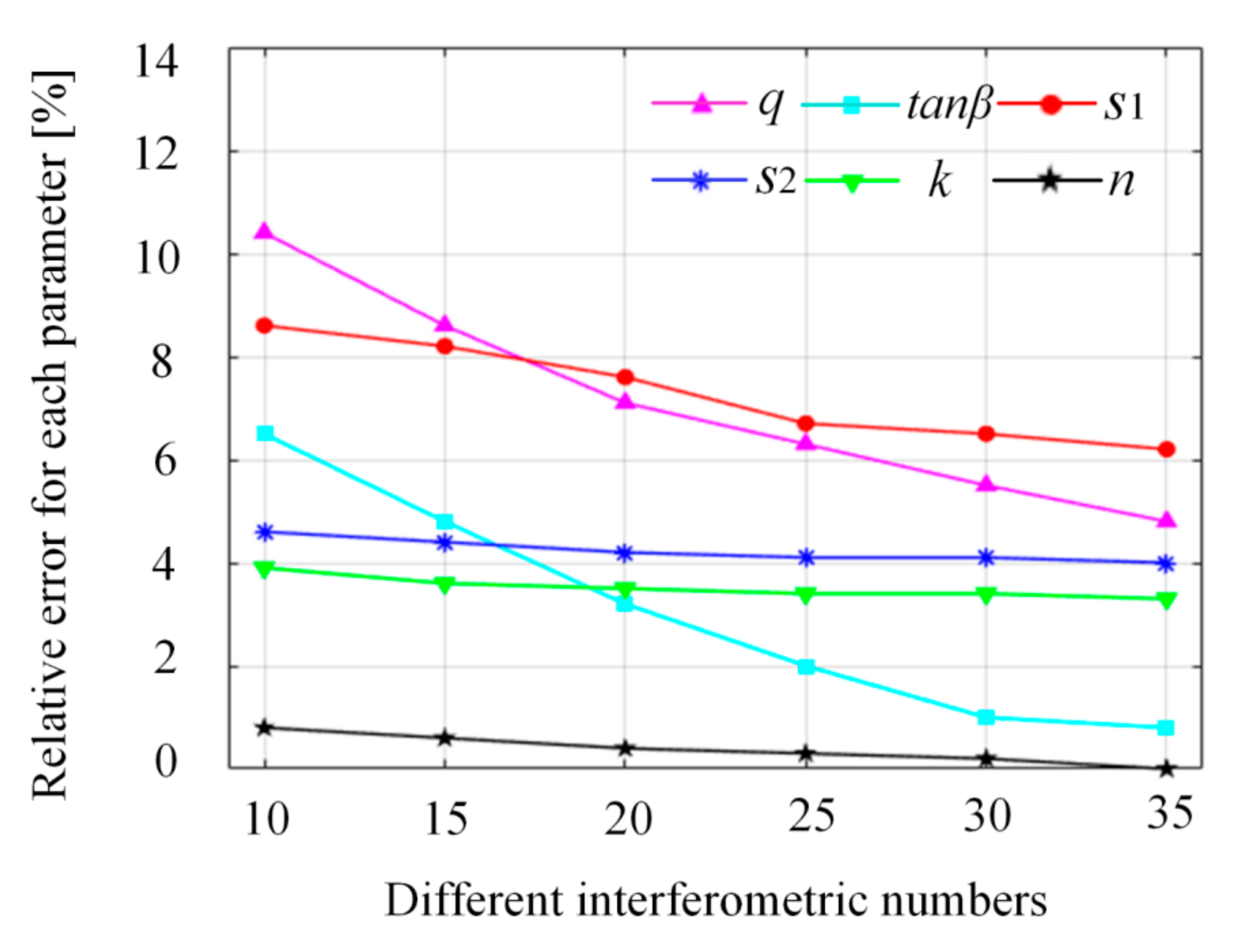
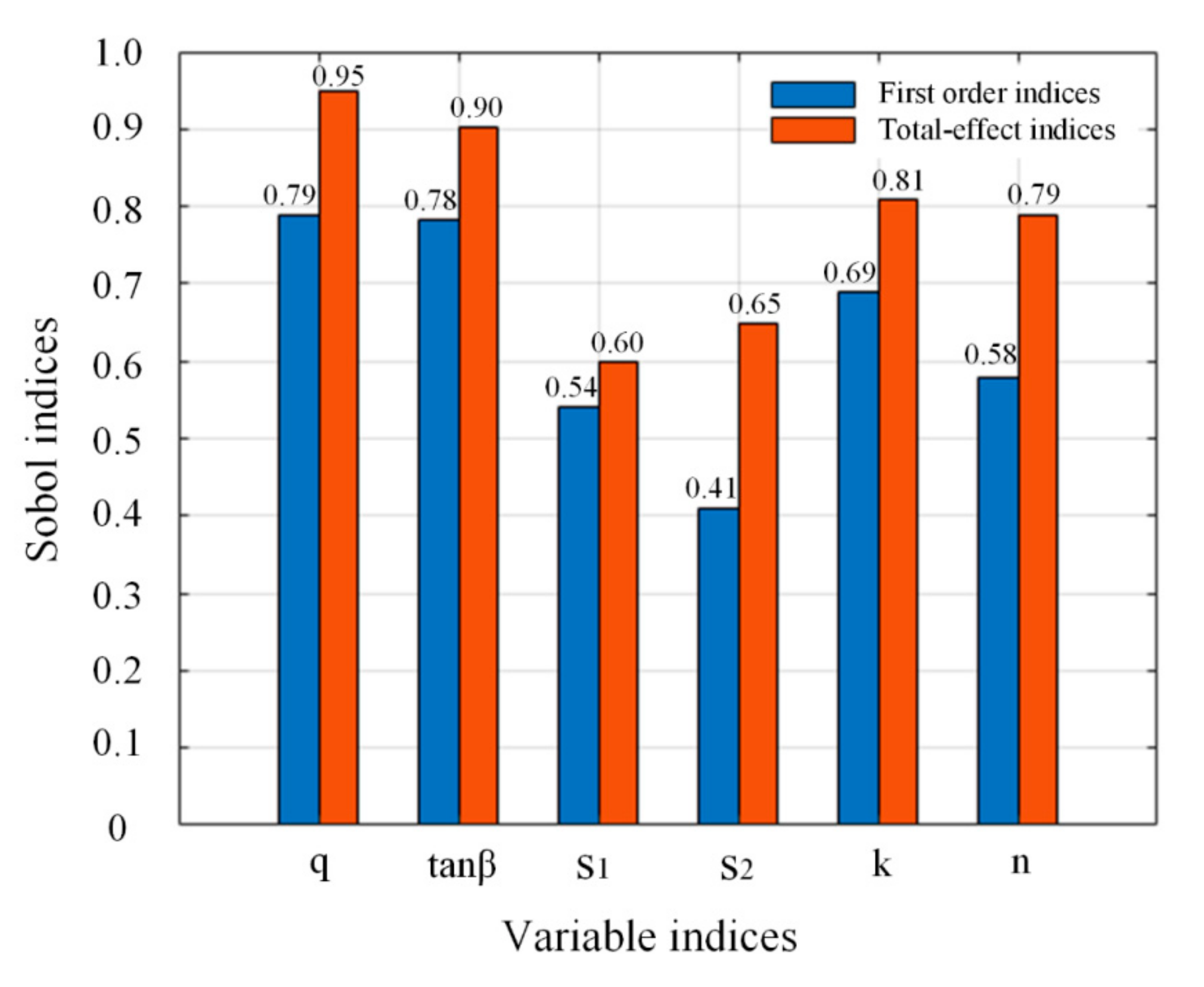
3.3.3. Sensitivity Analysis on CT-PIM Parameters

Since CT-PIM is directly used to predict the forward dynamic deformation subsequent to the SAR acquisitions, the accuracy of the predicted mining subsidence directly depends on the accuracy of CT-PIM parameters. Consequently, it is necessary to analyze the sensitivity of CT-PIM parameters. Sensitivity analysis can assist us in understanding how the parameters influence the predicted deformation, i.e., which parameter impacts the most and to what extent it impacts the results. The sensitivity analysis method based on Sobol indices is introduced here to execute a simulated experiment [39].
Sobol indices describe the correlation between each parameter and its global sensitivity on the objective function. The higher the sensitivity index, the higher the result error of the parameter on the deformation. Firstly, the objective function is decomposed based on variance analysis; then, the first-order indices ( S α , where α represents the certain parameter) and total-effect indices ( S α T o t ) of each parameter is calculated, and the sensitivity of the interactive input parameters can also be generated. Here, S α represents the partial variance, which describes the main contribution of a sample of the certain parameter for the output variances, while S α T o t represents the total variance, which describes the percentage of a group of samples for a certain parameter on the output variances. Finally, the disturbance analysis is used to quantitatively analyze the influences of different parameters on the final predicted deformation. The estimated two kinds of indices for each CT-PIM parameter are shown in Figure 18, where X axis represents the input parameters ( U P = [ q , t a n β ,   s 1 ,   s 2 ,   k ,   n ] ), and Y axis represents the Sobol indices for each parameter. The closer the magnitude of each corresponding Sobol index to 1, the higher sensitivity the parameter possesses. Table 6 lists the ranges of different importance extent. From it, we can determine that all the parameters are beyond the range of “Not correlated”, which implies their impacts on the accuracy of predicted deformation cannot be ignored. Among the six parameters, q and t a n β are more sensitive to the model, with the Sobol indices S α T o t of 0.95 and 0.90, respectively, which can be treated as “Very important” parameters. Consequently, we should pay more attention to the error control during the parameter estimation procedure for those two parameters. In contrast, s 1 and s 2 show relatively lower sensitivity than the remaining four parameters, with the Sobol indices S α T o t of 0.60 and 0.65, respectively. The two parameters can be treated within the united range of “Unimportant” and “Important”.

4. Discussion

Subsidence along the traverse and longitudinal lines marked in Figure 11c (EE’, FF’, GG’, HH’) were extracted for a profile analysis. The profile analysis results based on the SBAS-InSAR derived time series subsidence are shown in Figure 19 (as shown the dotted line), while the CT-PIM results are shown as Figure 19 (as shown the solid line). From the figures, we can see similar spatial-temporal characteristics and approximate same locations of pixels with separate subsidence bowls along EE’, FF’, GG’, and HH’, for both the two groups of generated results. The discrepancy between the SBAS results and CT-PIM predicted ones, in the case of Figure 19c (particularly in the black rectangle), was suggested to be related to the following reasons: (1) The systematic uplifts in the black rectangle in Figure 19c for the SBAS results were related to the residual atmospheric delay and orbital errors. During CT-PIM processing, the mining area was divided into several subsidence bowls artificially. (2) We treated the GG’ profile that only traversed a single subsidence funnel, and only one group of CT-PIM parameters was used to predict the subsidence. Some unrevealed deformation characteristics maybe hidden in the predicted results, which can be revealed by the SBAS-InSAR monitored results. As we determined for the InSAR-CTPIM derived results, the apparent three peak values were detected at 172 m, 322 m, and 414 m along EE’, with the subsidence of 232 mm, 249 mm, and 205 mm, respectively, and peak values at 149 m along the FF’ section of 219 mm, whereas, at 172 m, along GG’ of 218 mm and, at 80 m, along the HH’ of 247 mm. The multi peaks of the subsidence along traverse and longitudinal directions were due to the water-soluble mining activities with groups of drilling wells simultaneously.
Five feature points (F1–F5, marked in Figure 11c) are extracted for quantitative analysis, and the results are shown in Figure 20. It can be seen from Figure 20 that, during the whole period, the five feature points displayed similar temporal evolution trends: slow settlement period from 15 June 2015 to 29 March 2016, and then a rapid settlement period from 29 March 2016 to 15 August 2017. Maximum subsidence was determined at F5 with its accumulated settlement of 289 mm until 15 August 2017. In contrast, F1, which was far away from the wellhead, was relatively stable, with its maximum deformation accumulated to 98 mm until 15 August 2017. As introduced in Section 3.2.4, an 8-month temporal lag of the subsidence can be found in Figure 20, which is suggested to be mainly related to the dissolution processing of the mirabilite by the solvent, with a certain longer time from injection to the surface displacement emerged. In addition, the depth of rock salt mine is generally deeper than that of common coal mines, which also leads to the time delay from the underground displacement cavity being accumulated on the ground surface.
Another phenomenon of seasonal related variations was determined from our experiments. For a warm season (29 March 2016 to 19 October 2016 in Stage B and 12 March 2017 to 15 August 2017 in stage C), a rapid subsiding trend occurred for all the five feature pixels, with the cumulative maximum subsidence reaching up to 98 mm and 83mm, while, for a cold season (13 October 2015 to 29 March 2016 of Stage A and 19 October 2016 to 12 March 2017 of Stage B), a relatively slow developing trend dominated those points, with a maximum subsidence of 31 mm and 45 mm, respectively, for the two periods. The potential reasons are suggested to be related to the air temperature, which influences the dissolution rate of mirabilite. The higher temperature of warm periods can accelerate the dissolution, and, accordingly, increased the subsiding velocities. Comparatively, lower temperature in cold periods slowed down the dissolution processing, which induced a stable trend of deformation. It should be noted that the dissolution rate of mirabilite in water is directly affected by solvent temperature (as shown in Table 7); however, it is indirectly affected by the air temperature. Hot water is used as solvent in drilling soluble production, which is delivered from the processing plant to the injection well after being measured and distributed at the control station. In the process of transportation, the solvent temperature is easily affected by the outside air temperature, which supports the above temperature-related interpretations.
It can also be determined, in Figure 20, that four minor jumps occurred for all the five feature points (marked by black arrows). According to the precipitation and temperature information of the Hunan Lixian Meteorological Bureau, the precipitation increased significantly on 13 October 2015, 16 May 2016, 31 October 2016, and 28 Jun 2017, as shown in Figure 21 [41]. Besides the decrease of solvent solubility caused by the aforementioned low temperature in winter, an increase of rainfall also contributed to the recoveries of subsidence.

5. Conclusions

A novel InSAR deformation model, namely CT-PIM function, was proposed and applied for predicting the dynamic deformation over a drilling solution rock salt mine. The CT-PIM function was used as a substitute for traditional InSAR pure empirical models, which can also provide as potential combined use with other high-productive inspection methodologies, which has the following advantages: (1) with consideration of the physical underground mechanism, CT-PIM can describe the temporal dynamical characteristics of the mining-induced subsidence more realistically; (2) CT-PIM can be directly applied for the forward deformation prediction, which implements to the deficiency of non-consistency and unreasonableness between the traditional InSAR model (i.e., linear model or linear model combined with periodical function) and the forward prediction model (i.e., PIM); (3) it provides an alternative PIM parameters estimation method directly based on the InSAR phase observations, which can avoid the secondary error propagation from the InSAR inaccurate deformation to the subsequent deformation prediction; and, (4) as for the computational burden, since the GASM are based on the input InSAR unwrapped phases (not the final generated deformation sequences), we saved the preprocessing time for InSAR Geocoding compared to the static PIM.
The feasibility and improvement of our method was verified by both simulated and real-data experiments. The simulated results showed that the RMSE between the deformation results estimated by the new model and the simulated true value was ±4.5 mm, even under a high noise level of 0.65 rad. In the real data experiment, 32 Sentinel-1A SAR images were used to carry out the experiment over a water-soluble rock salt mine. As we determined, the maximum settlement was estimated as 294 mm. The experimental results were compared with external leveling results, and the RMSE was determined as ±10.9 mm, which accounts for only 6.9% of the maximum settlement. During the deformation prediction procedures, CT-PIM showed a considerable improvement of 32.7% than the traditional static PIM prediction approach, with an STD of ±12.9 mm compared to SBAS-generated results.

6. Patents

There are patents resulting from the work reported in this manuscript. Our research content has applied for a Chinese patent (ZL202010122691.8) entitled “A deformation monitoring method in mining area”.

Author Contributions

X.X. designed the experiments and produced the results; T.Z. carried out the experiment. X.X. and T.Z. analyzed the experiment results; L.C., X.L. and W.P. analyzed the precipitation data; X.X., W.P. and Z.Y. (Zefa Yang) helped to collect and analyze the leveling measurement in the real data experiment; X.L. and Z.Y. (Zhihui Yuan) contributed to the discussion of the results; X.X. and T.Z. drafted the manuscript. All authors have read and agreed to the published version of the manuscript.

Funding

This work was funded by the National Natural Science Foundation under Grant of China (Grant No. 42074033, 41904003, 41701536, 61701047); the Open Project Program of the Hunan Key Laboratory of remote sensing of ecological environment in Dongting Lake Area (Grant No. 2021-011); the Natural Science Foundation of Hunan Province, China (Grant No. 2019JJ50639, 2020JJ5571); and Key Project of Education Department of Hunan Province, China (Grant No. 18A148, 19C0042).

Data Availability Statement

The Sentinel-1 data presented in this study are openly available in ESA/Copernicus at https://scihub.copernicus.eu (accessed on 16 December 2021). The SRTM data presented in this study are openly available in the National Aeronautics and Space Administration (NASA, United States).

Acknowledgments

The Sentinel-1 A images used in this work are provided by the European Space Agency. Thanks for He Y.G. of Transportation Engineering College, Changsha University of Science and Technology, China, for providing the leveling deformation data of the research area, which provides available validation data for this work.

Conflicts of Interest

The authors declare no conflict of interest.

References

  1. Ministry of Natural Resources. China Mineral Resources Report; Geological Publishing House: Beijing, China, 2019; pp. 2–6. [Google Scholar]
  2. Zhang, M.G.; Wang, Z.S.; Wang, L.J.; Chen, Y.L.; Wu, Y.; Ma, D.; Zhang, K. Mechanism of collapse sinkholes induced by solution mining of salt formations and measures for prediction and prevention. Bull. Eng. Geol. Environ. 2019, 78, 1401–1415. [Google Scholar] [CrossRef]
  3. Buchignani, V.; Avanzi, G.D.; Giannecchini, R.; Puccinelli, A. Evaporite karst and sinkholes: A synthesis on the case of Camaiore (Italy). Environ. Geol. 2008, 53, 1037–1044. [Google Scholar] [CrossRef]
  4. Solari, L.; Montalti, R.; Barra, A.; Monserrat, O.; Crosetto, M. Multi-temporal satellite interferometry for fast-motion detection: An application to salt solution mining. Remote Sens. 2020, 12, 3919. [Google Scholar] [CrossRef]
  5. Wang, S.; Jiang, G.; Weingarten, M.; Niu, Y. InSAR evidence indicates a link between fluid injection for salt mining and the 2019 Changning (China) earthquake sequence. Geophys. Res. Lett. 2020, 47, e2020GL087603. [Google Scholar] [CrossRef]
  6. Furst, S.L.; Doucet, S.; Vernant, P.; Champollion, C.; Carme, J.L. Monitoring surface deformation of deep salt mining in vauvert (france), combining InSAR and leveling data for multi-source inversion. Solid Earth 2021, 12, 15–34. [Google Scholar] [CrossRef]
  7. Jung, J.; Kim, D.J.; Vadivel, P.S.K.; Yun, S.H. Long-term deflection monitoring for bridges using X and C-Band time-series SAR interferometry. Remote Sens. 2019, 11, 1258. [Google Scholar] [CrossRef] [Green Version]
  8. Tosti, F.; Gagliardi, V.; D’Amico, F.; Alani, A.M. Transport infrastructure monitoring by data fusion of GPR and SAR imagery information. Transp. Res. Procedia 2020, 45, 771–778. [Google Scholar] [CrossRef]
  9. Gagliardi, V.; Bianchini Ciampoli, L.; Trevisani, S.; D’Amico, F.; Alani, A.M.; Benedetto, A.; Tosti, F. Testing Sentinel-1 SAR interferometry data for Airport Runway monitoring: A Geostatistical Analysis. Sensors 2021, 21, 5769. [Google Scholar] [CrossRef]
  10. Zheng, M.; Deng, K.; Fan, H.; Du, S. Monitoring and analysis of surface deformation in mining area based on InSAR and GRACE. Remote Sens. 2018, 10, 1392. [Google Scholar] [CrossRef] [Green Version]
  11. Xiao, L.; He, Y.G.; Xing, X.M.; Wen, D.B.; Tong, C.G.; Chen, L.F.; Yu, X.Y. Time series subsidence analysis of drilling solution mining rock salt mines based on Sentinel-1 data and SBAS-InSAR technique. Int. J. Remote Sens. 2019, 23, 501–513. [Google Scholar]
  12. Ma, T.; Zhao, Y.J.; Zhang, W. Application of SBAS-InSAR technology in settlement monitoring of mining area. Geom. Spat. Inf. Tech. 2020, 11, 210–212. [Google Scholar]
  13. Chen, Y.; Tong, Y.X.; Tan, K. Coal mining deformation monitoring using SBAS-InSAR and offset tracking: A case study of Yu County, China. IEEE J. Sel. Top. Appl. Earth Obs. Remote Sens. 2020, 13, 6077–6087. [Google Scholar] [CrossRef]
  14. Yang, Z.F.; Li, Z.W.; Zhu, J.J.; Hu, J.; Wang, Y.J.; Chen, G.L. InSAR-Based model parameter estimation of probability integral method and its application for predicting mining-induced horizontal and vertical displacements. IEEE Trans. Geosci. Remote Sens. 2016, 54, 4818–4832. [Google Scholar] [CrossRef]
  15. Fan, H.; Lu, L.; Yao, Y. Method combining probability integration model and a small baseline subset for time series monitoring of mining subsidence. Remote Sens. 2018, 10, 1444. [Google Scholar] [CrossRef] [Green Version]
  16. Zhu, J.J. A Mining Monitoring Method Based on InSAR Technology. Chinese Patent ZL201310011306.2, 8 May 2013. [Google Scholar]
  17. Li, Z.W.; Yang, Z.F.; Zhu, J.J.; Hu, J.; Wang, Y.J.; Li, P.X.; Chen, G.L. Retrieving three-dimensional displacement fields of mining areas from a single InSAR pair. J. Geod. 2015, 89, 17–32. [Google Scholar] [CrossRef]
  18. Yang, Z.F.; Li, Z.W.; Zhu, J.J.; Preusse, A.; Yi, H.W.; Wang, Y.J.; Papst, M. An extension of the InSAR-Based probability integral method and its Application for Predicting 3-D Mining-Induced Displacements Under Different Extraction Conditions. IEEE Trans. Geosci. Remote Sens. 2017, 55, 3835–3845. [Google Scholar] [CrossRef]
  19. Yang, Z.F.; Li, Z.W.; Zhu, J.J.; Feng, G.C.; Wang, Q.J.; Hu, J.; Wang, C.C. Deriving time-series three-dimensional displacements of mining areas from a single-geometry InSAR dataset. J. Geod. 2018, 92, 529–544. [Google Scholar] [CrossRef]
  20. Xing, X.M.; Zhu, Y.K.; Yuan, Z.H.; Xiao, L.; Liu, X.B.; Chen, L.F.; Xia, Q.; Liu, B. Predicting mining-induced dynamic deformations for drilling solution rock salt mine based on probability integral method and weibull temporal function. Int. J. Remote Sens. 2020, 42, 639–671. [Google Scholar] [CrossRef]
  21. Wang, L.Y.; Deng, K.Z.; Zheng, M.N. Research on ground deformation monitoring method in mining areas using the probability integral model fusion D-InSAR, sub-band InSAR and offset-tracking. Int. J. Appl. Earth Obs. 2020, 85, 101981. [Google Scholar] [CrossRef]
  22. Xing, X.M.; Xiao, L.; Bao, L.; Chen, L.F.; Yuan, Z.H. An InSAR Prediction Method for Mining Subsidence in Drilling Water-Soluble Salt Mines. Chinese Patent ZL201910168502.8, 16 March 2021. [Google Scholar]
  23. Zhu, G.Y.; Shen, H.X.; Wang, L.G. Study of dynamic prediction function of surface movement and deformation. Chin. J. Rock Mech. Eng. 2011, 30, 1889–1895. [Google Scholar]
  24. Berardino, P.; Fornaro, G.; Lanari, R.; Sansosti, E. A new algorithm for surface deformation monitoring based on small baseline differential SAR interferograms. IEEE Trans. Geosci. Remote Sens. 2002, 40, 2375–2383. [Google Scholar] [CrossRef] [Green Version]
  25. Lauknes, T.R.; Zebker, H.A.; Larsen, Y. InSAR Deformation Time Series Using an L1-Norm Small-Baseline Approach. IEEE Trans. Geosci. Remote Sens. 2010, 49, 536–546. [Google Scholar] [CrossRef] [Green Version]
  26. Li, D.; Deng, K.Z.; Gao, X.X.; Niu, H.P. Monitoring and analysis of surface subsidence in mining areas based on SBAS-InSAR. Geom. Inf. Sci. Wuhan Univ. 2018, 43, 1531–1537. [Google Scholar]
  27. Zhang, Y.; Meng, X.M.; Jordan, C.; Novellino, A.; Dijkstra, T.; Chen, G. Investigating slow-moving landslides in the Zhouqu region of China using InSAR time series. Landslides 2018, 5, 1299–1315. [Google Scholar] [CrossRef]
  28. Wang, Q.M. Water-Soluble Salt Mine Mining and Design; Chemical Industry Press: Beijing, China, 2016; pp. 46–71. [Google Scholar]
  29. Yao, L.; Sethares, W.A. Nonlinear parameter estimation via the genetic algorithm. IEEE Trans. Signal Process. 1994, 42, 927–935. [Google Scholar]
  30. Xing, X.M.; Chang, H.C.; Chen, L.F.; Zhang, J.H.; Yuan, Z.H.; Shi, Z.N. Radar Interferometry Time Series to Investigate Deformation of Soft Clay Subgrade Settlement—A Case Study of Lungui Highway, China. Remote Sens. 2019, 11, 429. [Google Scholar] [CrossRef] [Green Version]
  31. Tian, Y.G. Study on Genetic Algorithm for Nonlinear Least Squares Estimation; Wuhan University Press: Wuhan, China, 2003. [Google Scholar]
  32. Xiao, H.F.; Tan, G.Z. Study on Fusing Simplex Search into Genetic Algorithm. Comput. Eng. Appl. 2008, 44, 30–33. [Google Scholar]
  33. Yang, Z.F.; Li, Z.W.; Zhu, J.J.; Yi, H.W.; Feng, G.C. Deriving Dynamic Subsidence of Coal Mining Areas Using InSAR and Logistic Model. Remote Sens. 2017, 9, 125. [Google Scholar] [CrossRef] [Green Version]
  34. Duan, M.; Xu, B.; Li, Z.W.; Wu, W.H.; Liu, J.H. Adaptively selecting interferograms for SBAS-InSAR based on graph theory and turbulence atmosphere. IEEE Access 2020, 99, 112898–112909. [Google Scholar] [CrossRef]
  35. Goldstein, R.M.; Werner, C.L. Radar interferogram filtering for geophysical applications. Geophys. Res. Lett. 1998, 25, 4035–4038. [Google Scholar] [CrossRef] [Green Version]
  36. Costantini, M.; Rosen, P.A. A generalized phase unwrapping approach for sparse data. In Proceedings of the IEEE International Geoscience and Remote Sensing Symposium, Hamburg, Germany, 28 June–2 July 1999; pp. 267–269. [Google Scholar]
  37. Li, Z.W.; Ding, X.L.; Zheng, D.W.; Huang, C. Least squares-based filter for remote sensing image noise reduction. IEEE Trans. Geosci. Remote Sens. 2008, 46, 2044–2049. [Google Scholar] [CrossRef]
  38. Fan, H.D.; Cheng, D.; Deng, K.Z.; Chen, B.Q.; Zhu, C.G. Subsidence monitoring using D-InSAR and probability integral prediction modelling in deep mining areas. Surv. Rev. 2015, 47, 438–445. [Google Scholar] [CrossRef]
  39. Cannavo, F. Sensitivity analysis for volcanic source modeling quality assessment and model selection. Comput. Geosci. 2012, 44, 52–59. [Google Scholar] [CrossRef]
  40. Ma, Z.Y.; Nie, C.X.; Wang, R.T. Geological Basis and Mining Technology of Well and Mineral Salt; National Mine Salt Industry Science and Technology Information Station: Chengdu, China, 1992; pp. 82–115. [Google Scholar]
  41. Fomelis, M.; Papageorgiou, E.; Stamatopoulos, C. Episodic ground deformation signals in Thessaly Plain (Greece) revealed by data mining of SAR interferometry time series. Int. J. Remote Sens. 2016, 37, 3696–3711. [Google Scholar] [CrossRef]
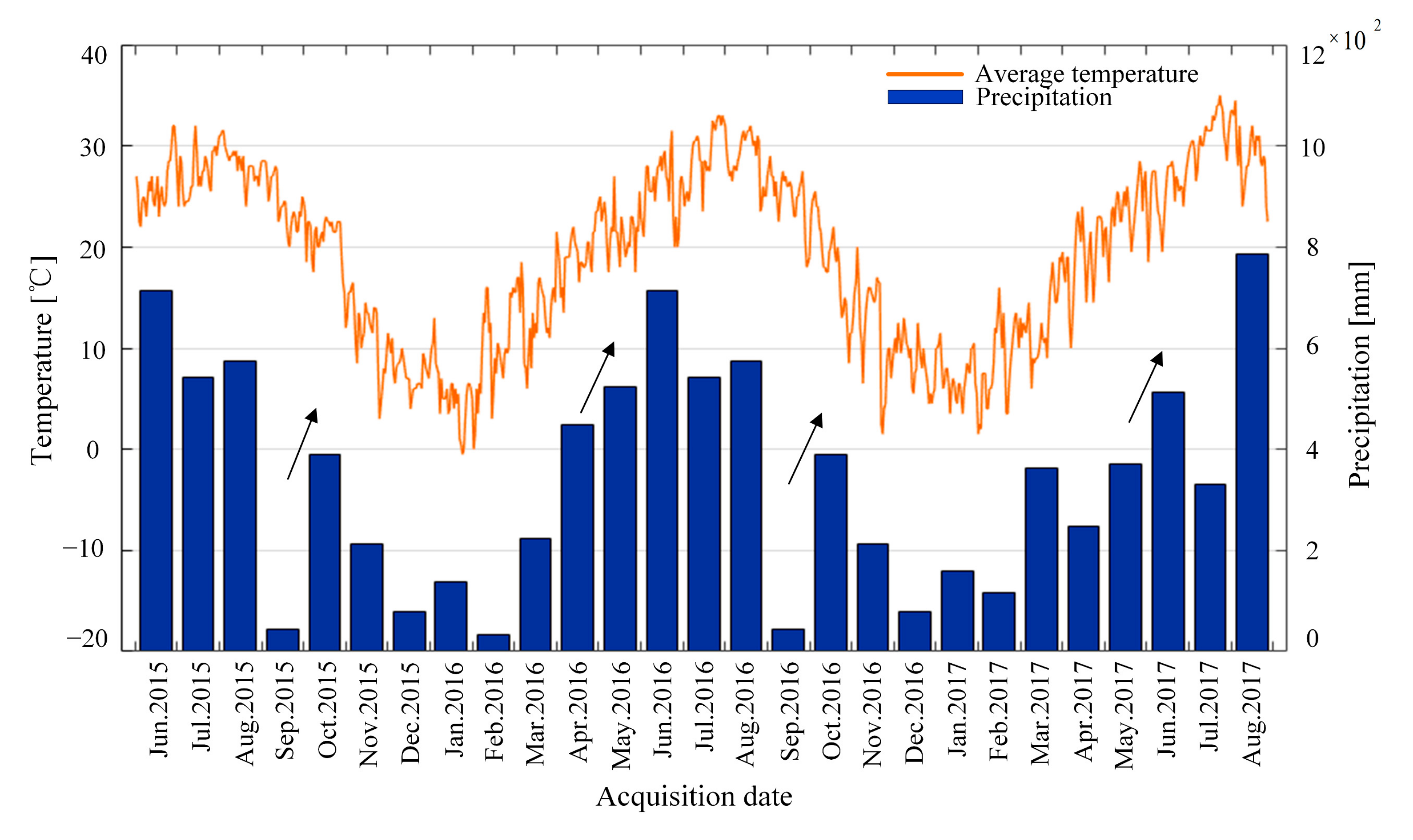
  42. Precipitation and Temperature Data of Lixian City, China. Available online: https://tianqi.911cha.com/lixian/2016.html (accessed on 15 December 2021).
Figure 1. Schematic diagrams for the coordinate system: (a) 3D view of the coordinate system; (b) profile along strike direction; (c) profile along dip direction.
Remotesensing 14 00842 g001
Figure 2. Flow chart of deformation prediction based on CT-PIM function.
Remotesensing 14 00842 g002
Figure 3. Selected images of simulated settlement field (at 24 d, 120 d, 288 d, 468 d, 528 d, and 576 d, respectively).
Remotesensing 14 00842 g003
Figure 4. Relative errors with different interferometric numbers under multi-master connection.
Remotesensing 14 00842 g004
Figure 5. Comparison between the CT-PIM generated deformation sequences (six periods are selected) and the simulated real settlement.
Remotesensing 14 00842 g005
Figure 6. Probability distribution for deformation deviations.
Remotesensing 14 00842 g006
Figure 7. Study area and SAR spatial coverage: (a) map of Hunan Province; (b) coverage of SAR images; (c) mean amplitude image of the study area.
Remotesensing 14 00842 g007
Figure 8. Field pictures of the residential area near the study area: (a) area with land salinization; (b) uneven displacement on the road; (c) cracks on the wall of a house; (d) a water pit in the salinized area.
Remotesensing 14 00842 g008
Figure 9. Schematic diagram of the lithological distribution over the study area.
Remotesensing 14 00842 g009
Figure 10. Spatio-temporal baselines.
Remotesensing 14 00842 g010
Figure 11. Schematic map of sub-settlement funnels distribution (with the settlement at 15 August 2017 generated via SBAS as the background): (a) the leveling points; (b) distribution of the seven sub-settlement funnels; (c) the distribution of the traverse-longitudinal profiles of the funnels; (d) 3D version of the mining coordinate system.
Remotesensing 14 00842 g011
Figure 12. Derived deformation sequences based on InSAR-CTPIM (reference date: 15 June 2015).
Remotesensing 14 00842 g012
Figure 13. Three-dimensional scenes of the predicted subsidence based on CT-PIM (reference date: 15 June 2015).
Remotesensing 14 00842 g013
Figure 14. Time series deformation at leveling points (reference date: 2 August 2015).
Remotesensing 14 00842 g014
Figure 15. Subsidence comparison: (a) SBAS-InSAR results; (b) CT-PIM predicted; (c) static PIM predicted (with reference to 15 June 2015).
Remotesensing 14 00842 g015
Figure 16. Differences of CT-PIM predicted subsidence with comparison of SBAS-InSAR results (with reference to 15 June 2015).
Remotesensing 14 00842 g016
Figure 17. Differences of static PIM predicted subsidence with comparison of SBAS-InSAR results (with reference to 15 June 2015).
Remotesensing 14 00842 g017
Figure 18. Estimated Sobol indices for CT-PIM parameter.
Remotesensing 14 00842 g018
Figure 19. Profile analysis based on SBAS (dotted line) and CT-PIM (solid line) predicted subsidence: (a) Profile EE’; (b) FF’; (c) GG’; (d) HH’.
Remotesensing 14 00842 g019
Figure 20. Time series settlement on feature points based on InSAR-CTPIM.
Remotesensing 14 00842 g020
Figure 21. Air temperature and precipitation of the mining area (6 June 2016 to 31 January 2017) [42].
Remotesensing 14 00842 g021
Table 1. Estimated CT-PIM parameters (under the 10 interferometric pairs).
ParametersSimulated
Real Value
CT-PIM
Generated Value
ErrorRelative Error
q 0.5040.5590.05510.4
t a n β 1.5601.6620.1026.4
s 1 ( m ) 30.31027.8012.5098.6
s 2 ( m ) 16.08015.3400.7404.5
k 0.5240.5040.0203.9
n 0.1670.1660.0010.6
Table 2. Estimated CT-PIM parameters (under the 35 interferometric pairs).
ParametersSimulated
Real Value
CT-PIM
Generated Value
ErrorRelative Error
q 0.5040.5280.0244.8
t a n β 1.5601.5720.0120.8
s 1 ( m ) 30.31028.4311.8796.2
s 2 ( m ) 16.08015.4370.6434.0
k 0.5240.5070.0173.3
n 0.1670.16700
Table 3. Geological parameters.
Geological
Parameters
m   ( m ) α   ( ° ) H   ( m ) D 1   ( m ) ω   ( ° ) v m   ( m / Day )
value35.7240258800.056
Table 4. Interferometric pairs and sensor parameters (Ascending, Orbit No. 11).
Image No.Acquisition Date (yyyy/mm/dd)Perpendicular
Baseline (m)
Temporal
Baseline (Days)
02015/06/1510.32−384
12015/07/0994.46−360
22015/08/028.65−336
32015/08/26−25.59−312
42015/09/19−27.87−288
52015/10/1342.76−264
62015/12/24125.03−192
72016/01/1719.96−168
82016/02/1099.87−144
92016/03/05−21.75−120
102016/03/29−48.25−96
112016/04/2237.12−72
122016/05/16−9.33−48
132016/07/0300
142016/08/2015.1548
152016/09/25−54.3284
162016/10/07−27.3396
172016/10/1963.93108
182016/10/3157.18120
192016/11/1252.15132
202016/11/2426.62144
212016/12/1825.12168
222016/12/3020.94180
232017/01/1176.93192
242017/02/1648.78228
252017/03/1234.61252
262017/04/05−16.41276
272017/04/2934.59300
282017/05/2347.07324
292017/06/2816.92360
302017/07/2263.26384
312017/08/15−69.95408
Table 5. Estimated CT-PIM parameters.
ParametersA1 A2 A3 A4 A5 A6 A7
q 0.8320.8820.9190.7410.9570.7500.974
t a n β 3.0603.1283.4733.3623.7323.6082.995
s 1   ( m ) 39.17040.69444.93349.88842.29747.46831.116
s 2   ( m ) 36.48138.63132.00139.81348.18447.37426.701
k 0.5180.6230.7430.6930.6580.7020.718
n 0.1500.1620.1820.1960.1450.1930.166
Table 6. Correlation extent for different ranges of sensitivity indices [39].
Correlation Extent Ranges of Sensitivity Indices
Very important0.8 <   S α   <   S α T o t   1
Important0.5 <   S α   <   S α T o t   0.8
Unimportant0.3 <   S α   <   S α T o t   0.5
Not correlated0 <   S α   <   S α T o t   0.3
Table 7. Seven groups of obtained InSAR-CTPIM parameters [28,40].
MineralTemperature (°C)
0102030405060708090100
Thenardite50.448.846.745.344.143.742.942.5
Glauber’s Salt5.09.019.440.8
Glauberite0.180.190.200.210.210.210.200.200.16
Publisher’s Note: MDPI stays neutral with regard to jurisdictional claims in published maps and institutional affiliations.

