
HyperLiteNet: Extremely Lightweight Non-Deep Parallel Network for Hyperspectral Image Classification


1
Key Laboratory of Intelligent Perception and Image Understanding of Ministry of Education of China, School of Artificial Intelligence, Xidian University, No. 2 South TaiBai Road, Xi’an 710071, China
2
School of Computer Science, Shaanxi Normal University, Xi’an 710062, China
*
Author to whom correspondence should be addressed.
†
These authors contributed equally to this work.
Remote Sens. 2022, 14(4), 866; https://doi.org/10.3390/rs14040866
Submission received: 30 December 2021
/
Revised: 24 January 2022
/
Accepted: 7 February 2022
/
Published: 11 February 2022
(This article belongs to the Topic Big Data and Artificial Intelligence)
Abstract
:Deep learning (DL) is widely applied in the field of hyperspectral image (HSI) classification and has proved to be an extremely promising research technique. However, the deployment of DL-based HSI classification algorithms in mobile and embedded vision applications tends to be limited by massive parameters, high memory costs, and the complex networks of DL models. In this article, we propose a novel, extremely lightweight, non-deep parallel network (HyperLiteNet) to address these issues. Based on the development trends of hardware devices, the proposed HyperLiteNet replaces the deep network by the parallel structure in terms of fewer sequential computations and lower latency. The parallel structure can extract and optimize the diverse and divergent spatial and spectral features independently. Meanwhile, an elaborately designed feature-interaction module is constructed to acquire and fuse generalized abstract spectral and spatial features in different parallel layers. The lightweight dynamic convolution further compresses the memory of the network to realize flexible spatial feature extraction. Experiments on several real HSI datasets confirm that the proposed HyperLiteNet can efficiently decrease the number of parameters and the execution time as well as achieve better classification performance compared to several recent state-of-the-art algorithms.
1. Introduction
With continuous improvement to the accuracy of image acquisition equipment, the spectral dimension of hyperspectral images (HSIs) has expanded greatly, which provides great discrimination ability for the component analysis of materials and land covers, etc. Therefore, the availability of abundant spectral–spatial information has allowed HSIs to be widely used in various applications, e.g., Earth observation [1], military reconnaissance [2], environmental protection [3], and resource management [4].
Numerous handcrafted features and traditional classifiers have been proposed over the past decades. However, HSI data suffers from the “curse of dimensionality” problem, due to the extremely limited hyperspectral training samples [5]. Therefore, many linear and nonlinear dimension reduction algorithms, such as band selection [6], principal component analysis [7], independent component analysis [8], and the maximum noise fraction [9] have been proposed to address this problem. Such algorithms employ feature optimization to remove redundant features and improve classification performance. Traditional classifiers can be mainly divided into two categories, according to their feature extraction characteristics: (1) spectral-based classification algorithms, such as support vector machines (SVM) [10], K-nearest neighbor [11], multinomial logistic regression [12], and random forest [13]; (2) spectral–spatial-based classification algorithms, e.g., SVM with composite kernels (SVMCK) [14], sparse representation-based classifiers [15], spatial–spectral derivative-aided kernel joint sparse representation [16], and adaptive nonlocal spatial–spectral kernels [17]. However, above-mentioned algorithms usually adopt handcrafted features in terms of the requirements of professional domain knowledge in the HSI classification area.
In contrast, deep learning (DL)-based algorithms demonstrate automatic representative and abstract feature extraction due to the rapid iteration and GPU-based parallel implementation. In the remote sensing field, DL-based algorithms also demonstrate extremely promising results. For instance, the stacked autoencoder [18] demonstrates the effectiveness of DL models in abstract high-level semantic feature extraction. The restricted Boltzmann machine and deep belief network [19] and unsupervised greedy learning algorithms realize the DL of objects. With the development of DL, convolutional neural networks (CNN) are widely used in HSI classification tasks. For example, Zhong et al. proposed the spectral–spatial CNN-based algorithm (SSRN) [20] by combining 3D convolutions and residual connections to realize robust HSI classification results. To refine the feature fusion process, Gao et al. [21] performed multi-scale feature extraction and dense feature fusion to expand the features of different levels and scales. Li et al. [22] proposed a hierarchical homogeneity–attention network to consolidate the position supervision of object regions and accelerate computation by reducing the number of similar operations. In terms of the visual invariance of the CNN, input image visual transformation causes drastic fluctuations in network performance. To address the issue of insufficient spectral–spatial feature extraction, Zhang et al. [23] proposed a spectral–spatial attention fusion with a deformable convolution residual network. The capsule network (CapsNet) was proposed [24] to improve network robustness and preserve more efficient position information that is omitted in traditional CNNs. Then, the deep convolutional capsule neural network (DC-CapsNet) [25] introduced CapsNet in 3D convolution to enhance the robustness of the learned spectral–spatial features. The generative adversarial network (GAN) has recently demonstrated satisfying performance for alleviating the problem caused by an insufficient number of labeled samples of CapsNet. However, it is difficult for GAN to model and preserve the relative positions between features accurately. To eliminate the mode collapse and gradient disappearance problem caused by traditional GANs, Wang et al. [26] developed a dual-channel spectral–spatial fusion capsule GAN (DcCapsGAN) by integrating CapsNet with a GAN. The progress of DL-based algorithms also exposed some challenging issues. With the expansion in complexity of DL networks, though the performance improved dramatically, the requirement of training samples and depths increase proportionally with the complexity of the model and make it difficult to deploy on edge devices. Therefore, realizations of an efficient DL structure with lower time costs and fewer training samples are more requisite for improving the HSI classification performance; it is a more crucial and applicable research task for mobile devices and in-orbit aerospace applications.
Recent research has revealed that neural networks with deep structures typically exhibit higher nonlinearity capabilities and stronger function approximations when automatically learning more abstract features [27]. However, deeper network structures also give rise to the vanishing and exploding gradient problems. Recent studies have indicated that a class of widened ResNets is far superior than their deep counterparts [28]. Shallow network structures with high parallelizations tend to provide fast responses and low latency. In addition, Wu et al. proved that a well-designed shallow neural network can outperform many deep neural networks [29], and recent empirical work has further indicated that obtaining the best accuracy requires a balance of depth and width [30]. However, most of these previous studies only focused on networks with linear and sequential structures. Conversely, in [31], it is found that the performance of a shallow network with a parallel structure is similar to that of the deep network. Therefore, compared to deep networks with more sequential processing and higher latency, the parallel shallow networks are more suitable for the hardware applications and deployment [31].
On the other hand, compressing a well-trained complex model or learning a lightweight model with carefully designed network structures are the current mainstream methods to handle the network efficiency problem caused by CNN-based algorithms. Network operating efficiency is primarily affected by the following four components: the number of parameters, the number of computations, memory access, and memory usage. The main design principle of a lightweight network architecture model can be mainly divided into the convolutional level, the convolution operator level, and the computation method:
(1) In the convolutional level: Redesigning the convolutional level primarily involves small-size convolution kernels, a bottleneck layer, and channel concatenation. For example, SqueezeNet [32] replaces convolution with convolution, reduces the number of input channels in the squeeze layer, and concatenates two sets of convolution output channels to obtain the target number of output channels to reduce network complexity.
(2) In the convolution operator level: Standard convolution has the inherent properties for global spacial and channel feature extraction. ShuffleNet V1 [33] limits the convolution operation to each group and performs a channel shuffle to promote the flow of information between groups. This is equivalent to decomposing the global channel feature extraction process into a local channel feature extraction and channel shuffle process. Furthermore, the depthwise separable (DW) convolution completely separates the space and channel feature extractions. From the implementation perspective, DW convolution can be considered as a special case of group convolution. The MobileNet family has successfully applied DW convolution and recently made a series of improvements [34,35,36]. Subsequently, different from DW convolution, Ghost [37] performs a one-to-many mapping output of a single feature map. In addition to channel decomposition, standard convolution can be further decomposed in spatial dimensions. For example, Zhang et al. [38] developed a compact convolution module to divide the input feature maps into groups and perform cyclic recursive feature extraction in each group. Compared to the channel-specific and spatially-agnostic nature of convolution, Involution [39] involves a spatially-specific and channel-agnostic operation that is distinct in the spatial extent but shared across channels. However, extremely low computational costs are likely to cause significant performance degradation. To address this problem, MicroNet [40] integrates sparse connectivity into convolution and constructs a dynamic activation function, i.e., dynamic shift max.
(3) In the computation level: Current CNNs primarily rely on multiplication operations, which are more computationally complex than addition operations. To address this issue, AdderNets [41] replaces massive number of multiplication operations in CNNs with less-expensive addition operations to reduce computational costs. Note that most of the aforementioned algorithms are based on the parameter and computation as model design indicators, and the actual acceleration effect is inferior to the theoretical analysis value. Shufflenet V2 [42] deeply analyzes the influence of different elements, e.g., memory access cost. Therefore, in addition to theoretical indicators, more attention should be paid to the actual time costs on equal hardware. The superiority of the lightweight structures has also been confirmed in the HSI classification tasks. Zhang et al. [43] proposed 3-D-LWNet, which has a deeper network structure and exhibits better classification performance than conventional 3D-CNN models. In addition, LWCNN [44] employs spatial–spectral Schroedinger eigenmap (SSSE)-based feature extraction and a dual-scale convolution module. The former reduces dimensions, and the latter address the SSSE features from a 1D vector viewpoint to reduce the number of parameters. Based on the conclusions of a neural architecture search [45], LMAFN is proposed to combine Ghost and ECA modules for further achieving efficient feature extraction performance [46]. LiteDepthwiseNet [47] used 3D depthwise convolution to reduce the number of parameters as well as remove the ReLU layer and batch normalization layer in the original 3D depthwise convolution to improve the overfitting phenomenon of the model on small-sized datasets.
Considering that compact lightweight models still achieved comparable or even better performance with fewer parameters, a lightweight model indicates more effective representative knowledge capacity than traditional DL models. However, blindly reducing model size can easily lead to knowledge degeneration, which contradicts the purpose of the lightweight design. To address this issue, CondConv [48] embeds multiple sets of convolution kernels in the convolutional layer and adaptively combines the weights according to the input, which is equivalent to learning specialized convolutional kernels for each example in terms of increasing network capacity while maintaining inference efficiency. To reorganize multiple sets of static convolution kernels according to the input, DYNet [49] performs a low-redundancy and efficient dynamic convolution to avoid redundant calculations and similar feature generation while maintaining a lightweight structure and efficient inference ability. Moreover, the study finds that dynamic networks can address domain conflicts by aggregating residual matrices and a static convolution matrix [50].
In the HSI classification area, the limited availability of labeled samples hinders the classification accuracy and optimization performance of DL. Therefore, recently, few-shot learning [51], domain adaptation [52], transfer learning [53], and meta learning [54] have been gradually proposed to address this issue. For example, Li et al. [55] proposed DCFSL, which utilizes a conditional adversarial domain-adaptation strategy to overcome domain shift and achieve domain distribution alignment. In addition, AMF-FSL [56] transfers the learned classification capabilities from multiple source data to the target data. To realize the promising performance with limited labeled samples, the above DL methods are generally based on complicated network structures and learning strategies. Therefore, an efficient network model that can obtain effective classification results with limited labeled samples is required. Intuitively, a lightweight model can also mitigate the requirements for the quantity of labeled samples to a certain extent.
Based on the above-mentioned knowledge, and aiming at realizing high efficiency and performance at lower computation cost, a HyperLiteNet is proposed and designed in this paper, which is an extremely lightweight non-deep parallel network. In the proposed HyperLiteNet, a parallel shallow narrow network is constructed to reduce network complexity and execution cost, where a parallel dual-branch structure is employed to enhance the nonlinearity of network and the capability of feature extraction. In addition, the spatial features and spectral features are extracted via a parallel dual-branch structure to, respectively, promote the diversity and divergence of the extracted features. As the main components of the dual-branch structure, lightweight pointwise convolution units and lightweight dynamic convolution units are constructed to further reduce the network’s complexity. In addition, the introduction of dynamic modules enables more elastic mapping with the input sample to generate compact and representative features. The experimental results confirm that the proposed HyperLiteNet outperforms other comparison algorithms with an extremely low number of parameters and high execution efficiency.
The remainder of this paper is organized as follows. Section 2 presents the proposed HyperLiteNet in detail. Experimental validation of the proposed HyperLiteNet compared to existing algorithms, including parameter analysis, classification results, classification efficiency, and accuracies, are presented in Section 3. Some experimental results are discussed in Section 4. Finally, conclusions are presented in Section 5.
2. Proposed Methods
The overall framework of the proposed HyperLiteNet is shown in Figure 1. The proposed HyperLiteNet can be roughly divided into five main components: (1) the parallel interconnection module (PIM); (2) the pointwise convolution branch (PCB) to extract spectral features; (3) the dynamic convolution branch (DCB) to extract spatial features; (4) the feature interconnection module (FIM); (5) the classification module (CM). In summary, the specific spectral and spatial features are extracted independently by the PCB and the DCB, respectively. Then, the spectral–spatial features are fused by the FIM and classified by the CM module. The details of different components are illustrated in the following parts.
2.1. Parallel Interconnection Module (PIM)
The PIM is the primary component of the proposed HyperLiteNet, where the parallel structure contains more nonlinear activation layers than a serial structure at the same depth. The paralleled shallow structure realizes an efficient nonlinear activation ability to extract abstract high-level features through utilizing PCB and DCB structures. With the reduced network depth, the vanishing and exploding gradient problems are mitigated in the PIM. This dual-branch structure is adopted to extract abstract spectral and spatial features independently and in a parallel manner through an extremely shallow network structure. As a result, due to the task decomposition of the PCB and DCB, fewer channels are established by the PIM in each branch than traditional spectral–spatial combination networks. Therefore, the network structure can be efficiently compressed in a compact, parallel manner with a lighter structure and better feature extraction. The structure of the PIM is mainly composed of three stages (), which extract shallow pixel-level features, mid-level features, and deep high-level features, respectively. The features extracted in each stage are fused at the tail of each stage and then input to the next stage to further increase the discriminativeness of the extracted features. Meanwhile, each stage contains two pointwise convolution (PW) units and one depthwise separable dynamic convolution (DC) unit. In the feature extraction process, the PCB and DCB comprise lightweight PW and DC units, respectively. Therefore, the spectral and spacial feature can be extracted in a parallel manner to accelerate execution efficiency. Further, for combining and fusing the spectral and spatial features at different stages, the FIM is designed to connect each stage to the subsequent stage. The entire structure provides a compact and efficient parallel method to extract and fuse the spectral and spatial features with a small number of parameters and low computational cost.
2.2. Pointwise Convolution Branch (PCB) and Dynamic Convolution Branch (DCB)
2.2.1. Pointwise Convolution Branch (PCB)
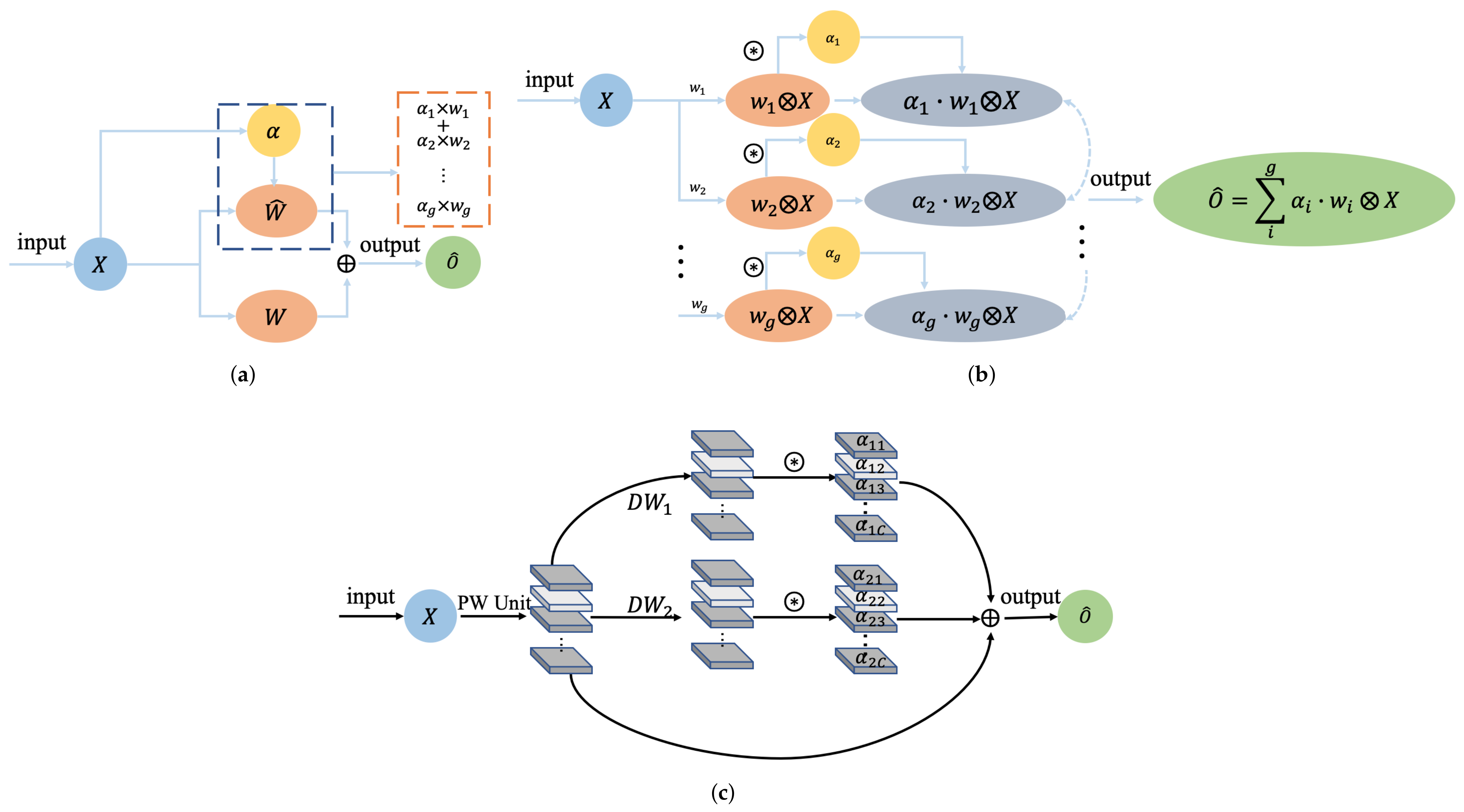
As shown in Figure 2a, lightweight PW units are employed in the PCB to extract spectral features. Here, only continuous spectral features are processed at a certain point in the feature map. The PCB is concentrated to effectively extract spectral distinguishing features. The pointwise (PW) convolution is calculated as follows:
where is the spectral vector at the of the input features. is the c-th PW convolution to convolve with for obtaining the output , where is the value at in the c-th channel of the output. It can be seen from the calculation process that the PW convolution is essentially a weighted summation of the spectral vectors of the input features. The procedure intensifies the channels that contributed more discriminant information with a dynamic learning process, which can indicate more satisfying effects and efficiency than traditional band-selection algorithms.
2.2.2. Dynamic Convolution Branch (DCB)
In traditional convolution, all input samples are treated equally to the convolution kernel, and the parameters of the convolution kernel are determined after the training process in a static network manner. Differing from static networks, dynamic networks attempt to adjust the network structure adaptively and dynamically according to the varied inputs. Therefore, for different inputs, a dynamic network can deform the network structure corresponding to the local areas, which efficiently improves the robustness and knowledge capacity of the network with low latency. The introduction of a dynamic network enables a more elastic mapping. Define the network convolutions in Figure 3a as follows:
where and are the static convolution kernel and the dynamic convolution kernel, respectively. and are the number of input channels and the number of output channels. If is ignored, is equivalent to .
The structure of the standard dynamic convolution is shown in Figure 3b, where the multi-group parallel standard convolutions extract features independently. Then, the extracted features are adjusted dynamically through each attention dynamic unit. The multi-group features are dynamically fused by a dynamic fusion unit. Essentially, the dynamic fusion unit reorganizes multi-group standard dynamic convolutions with different weights. The standard dynamic kernel can be generated by the following formulas:
where and are the output channels and number of static convolution kernel groups, respectively. represents the importance weights of different sets of static convolution kernels based on the input. indicates the c-th convolution kernel of the i-th static convolution. Based on the linear combination characteristic of convolution, the dynamic convolution output can be mathematically represented as:
where the output of the dynamic convolution kernel can be expressed as a linear combination of the output of the static convolution kernel.
Further, for realizing the design of the lightweight structure, we adopt the lightweight DW dynamic convolution as the primary component of the DC unit in Figure 3c. Specifically, the parameter definition is different in the realization of the DW dynamic convolution. indicates the c-th channel of the i-th static DW convolution due to the characteristic of DW convolution. Compared with the standard dynamic convolution, DW dynamic convolution realizes the single-channel-level dynamic fusion to further decompose and refine the dynamic convolution. In addition, we further analyze the DW dynamic convolution from the perspective of parameters and calculations. Assume the standard convolution and the DW dynamic convolution . The PW convolution adjusts the number of channels in the DW dynamic convolution. Ignoring the input adaptive correlation calculation, the reduced computation and parameters effect can be written as follows:
where s is the space size of the feature map.
Compared to the traditional standard convolution, the diversity and spatial differences of the spatial characteristics can be extracted flexibly and enhanced by the dynamic module. In addition, the DCB realizes the potential for reducing the number of parameters and computations, which improves the efficiency of the network operations.
2.3. Feature Interconnection Module (FIM) and Classification Module (CM)
The function of FIM is to fuse the spectral and spatial features of the two branches and feed the fused features to the next stage of the network. Here, suppose the input spectral and spatial features in are defined as and , respectively. The calculation process of FIM is determined by the following formula:
For the CM, the PW unit progressively reduces the number of channels and prevents the sharp reduction in the number of channels for avoiding the feature information loss. In this module, we utilize cross entropy as the loss function for HSI classification. The cross entropy loss can be represented as:
where C indicates the number of classes, and are the truth and predicted labels, respectively, and N is the number of samples in a minibatch.
3. Experiments and Analysis
In this section, we mainly evaluate our proposed frameworks on three real HSI datasets. The experimental settings and results, including parameters analysis and evaluation metrics are illustrated. Finally, the comparison result with the existing algorithms are analyzed and discussed in this section.
3.1. Datasets Descriptions
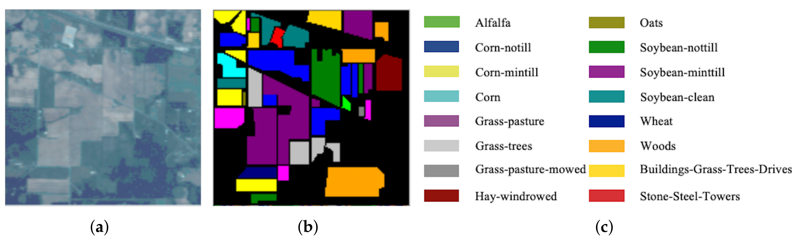
The Indian Pines (IN) dataset was captured in 1992 over the Indian Pines agriculture experimental area by the Airborne Visible/Infrared Imaging Spectrometer (AVIRIS) sensor. The IN dataset has 220 bands with a wavelength range from 0.4 to 2.5 m, and with pixels. Note that 20 bands of noisy or water-absorption regions are removed in our experiments. The IN dataset contains 16 different ground-truth classes. The three-band false-color composite of the IN images and the corresponding ground-truth data are shown in Figure 4.
The University of Pavia (UP) dataset was collected in 2001 over the Pavia university campus through the Reflective Optics System Imaging Spectrometer (ROSIS). The UP dataset has 115 bands with a wavelength range from 0.43 to 0.86 m, and with pixels. Note that 12 bands of noisy or water-absorption regions are removed in our experiments. The UP dataset contains nine different ground-truth classes. The three-band false-color composite of the IN images and the corresponding ground-truth data are shown in Figure 5.
The Salinas (SA) dataset was gathered over the Salinas Valley in California by the AVIRIS sensor. The SA dataset has 220 bands with a wavelength range from 0.36 to 0.5 m, and with pixels. Note that 20 bands of noisy or water-absorption regions are removed in our experiments. The SA dataset contains 16 different ground-truth classes. The three-band false-color composite of IN images and the corresponding ground-truth data are shown in Figure 6.
3.2. Experimental Configuration and Parameter Analysis
3.2.1. Experimental Configuration
The experimental configuration is as follows: an Intel Xeon W-2123 CPU at 3.60 GHz with 64-GB RAM and an NVIDIA GeForce GTX 2080 Ti graphical processing unit (GPU) with 11-GB RAM were used. The software environment includes a 64-bit Windows 10 system and the Pytorch 1.6.0 DL frameworks. Here, the learning rate is set to 0.0001, and the Adam optimizer is used with a batch size of 72. In addition, five labeled samples are randomly selected from each class as a training set for each HSI. To avoid the inclination in random sampling, the evaluated mean value is reported for parameter analysis and classification result comparison with ten random repetitions.
3.2.2. Experimental Parameter Analysis
To evaluate the effectiveness of the proposed HyperLiteNet, we mainly evaluate the effect of the number of kernels (extracted channels), the quantity of parameters, and the training epoch. We first analyze the effect for the number of kernels in each conventional layer. The number of kernels in each layer is selected from for each dataset. The effect analysis results are illustrated in Figure 7a,b; we can notice that the number of 16 kernels, corresponding to the least number of parameters, presents the worst performance for all experimental datasets. The overall accuracy (OA) gradually increased with the increasing number of channels. Compared to 128 channels, we observe from Figure 7a that 16 channels obtain lower OA with the same number of training epochs (4000). It is notable that the increasing number of channels can improve the classification accuracy significantly. However, when the number of convolution kernels exceeds a certain threshold, the performance gradually increases to a stable value. The excessive number of convolution kernels brings additional an parameter burden without beneficial effects on performance. The aforementioned data analysis indicates that the limited model performance and difficult model optimization phenomenon exist in low-parameter models. Therefore, the optimal parameters acquired from the above-mentioned analysis are utilized in the following comparison experiments.
Because of the correlation between time costs and model convergence, we evaluate OA under different numbers of training epochs to achieve a balance between time costs and performance, where training epochs are a varied set from 50 to 4000 with step 200. The analysis results are presented in Figure 7c. We can notice that the proposed model reaches a stable and exceptional OA after 2000 epochs. Moreover, MiniNet achieves acceptable results in 1000 epochs. Considering the necessity of adequate training, 4000 is chosen as the number of training epochs in the following experiment.
3.3. Ablation Study for DW Dynamic Convolution
To verify the proposed effectiveness of the DW dynamic convolution (DC), we compare the proposed DC with standard convolution (SC) ( convolution kernel is applied), and multi-scale convolution (MSC) ( and convolution kernels are applied). The comparison results are illustrated in Table 1. It is obvious that the DC improves the classification performance while effectively compressing the model size. In addition to quantitative analysis, the t-SNE feature visualization technology is further exhibited to qualitatively analyze the differences between the three convolutions in Figure 8. The blue dotted line indicates the comparison between DC and SC, and the red dotted line represents the comparison between DC and MSC. From Figure 8a–c, we can observe that the dotted line in Figure 8a has a higher concentration and purity ratio. This phenomenon also appeared in Figure 8g–i. The red dotted area in Figure 8d,g exhibits better concentration than Figure 8f,i. Moreover, it is roughly observed that the distinction between the red and green cluster in the blue dotted rectangle region for Figure 8d is inferior to Figure 8e. Meanwhile, in real classification investigations, there are many misclassified samples in these two classes for Figure 8d,f, which further indicates that these two classes are more indistinguishable in real classification tasks. Overall, from the t-SNE feature visualization, as illustrated in Figure 8, the DC achieves a more distinguishable and recognizable feature extraction capability.
3.4. Classification Accuracy and Performance
In this part, we compare the proposed HyperLiteNet with six comparable methods: two traditional methods, SVM and SVMCK, and four deep learning-based methods, SSRN, LMAFN, DcCapsGAN, and DCFSL. The SVM only extracts spectral features, and the SVMCK further introduces spatial features for classification. The SSRN is a classic method using 3D convolution for HSI classification. The DcCapsGAN combines the capsule network and GAN to enhance the model robustness. Based on the lightweight characteristics of the proposed HyperLiteNet, we also compared it with the LMAFN. In order to test the effectiveness of proposed HyperLiteNet under the condition of limited labeled samples, we further compared the proposed HyperLiteNet with the few-shot learning method DCFSL. The quantitative experimental results of different methods are shown in Table 2, Table 3 and Table 4. The metrics include overall accuracy (OA(%)), average accuracy (AA(%)), kappa (KP(%)), the number of parameters (PA), floating point operations (FLOPs (M)), training time (Train(s)), and test time (Test(s)).
From Table 2, Table 3 and Table 4, we can observe that, in most cases, the accuracy of SVM and SVMCK are inferior to DL-based methods. In terms of the spectral–spatial information involved in SVMCK, which presents higher classification accuracy than SVM, data-driven characteristics and nonlinearity fitting of CNNs can approximate any function, which facilitates the extraction of discriminant features. Therefore, most of the DL-based models in this paper perform better than traditional SVM and SVMCK methods. The implementation of 3D convolution is consistent with the continuity of the HSI spectral curve. Therefore, the SSRN obtains relatively stable classification performance on most datasets. Our previous research work presents LMAFN based on a lightweight design, which achieves the best operating efficiency among all comparable DL-based methods. The ingenious combination of the GAN and capsule network promotes the robustness of the DcCapsGAN. However, the huge number of parameters in the capsule network also becomes a significant burden for DcCapsGAN. The DCFSL obtains acceptable numerical indexes with low efficiency based on conditional adversarial domain daptation strategy. Compared with LMAFN, we can observe from Table 2, Table 3 and Table 4 that the proposed HyperLiteNet further compresses the quantity of parameters and greatly improves network efficiency, which is beneficial to the deployment of the HyperLiteNet on edge devices. Meanwhile, the feature extraction capabilities of the HyperLiteNet support satisfactory classification results with limited labeled samples. Generally, the proposed HyperLiteNet achieves the optimal classification accuracy among all comparison methods with the lowest number of parameters and execution costs.
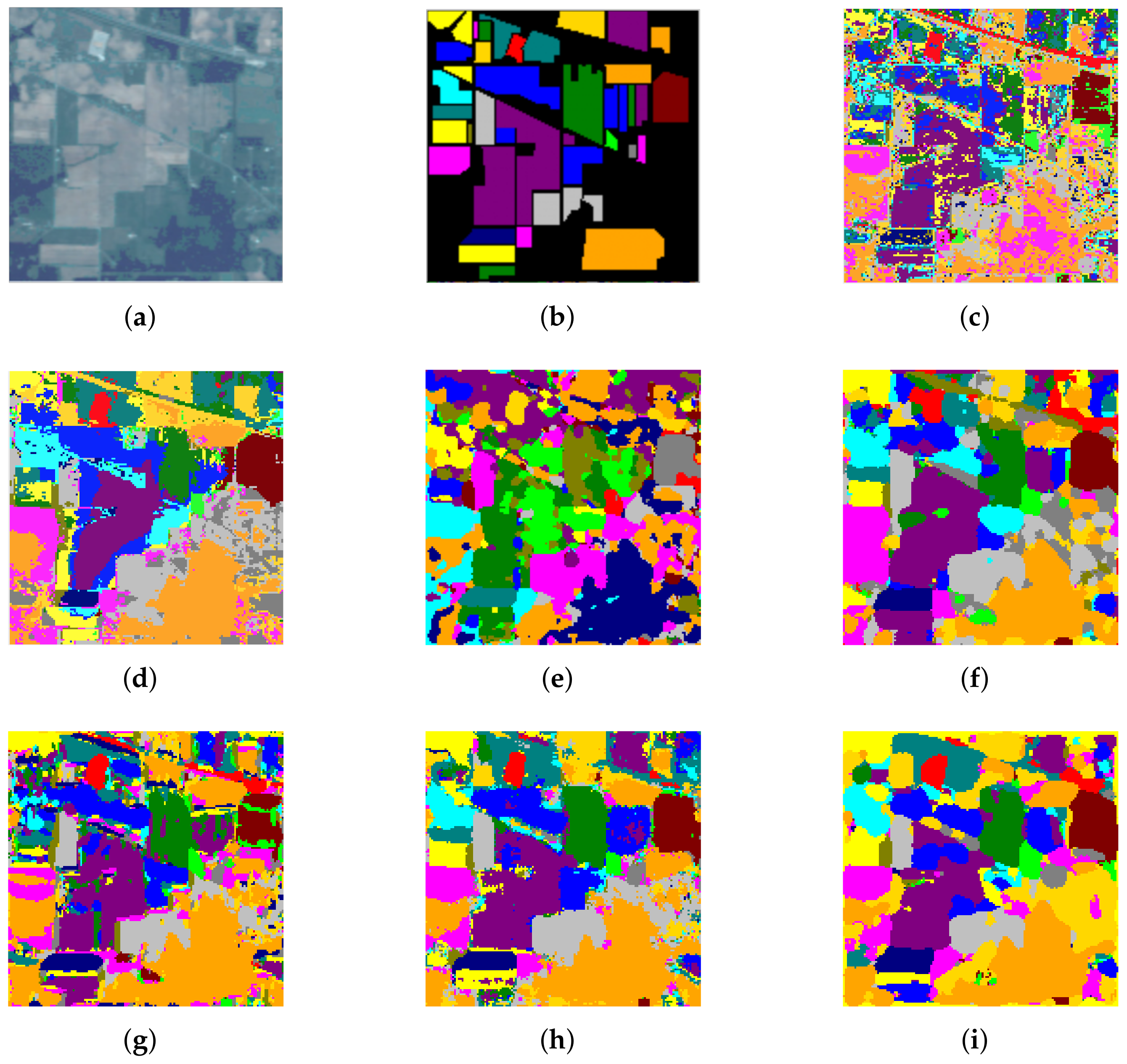
The qualitative comparisons of the classification maps for different algorithms are illustrated in Figure 9, Figure 10 and Figure 11. In our expectation, due to the lack of spatial information, SVM indicates the most random misclassified noise labels on the three datasets. In contrast, other methods that exploit spectral–spatial combination information present smoother classification maps than SVM. In addition, the SSRN and DcCapsGAN have more distinguishable classification boundaries based on more elaborately designed structures involved in the structure, whereas the number of parameters also increased dramatically. We can further observe that the HyperLiteNet produces a smoother classification area compared with other comparison algorithms in the red dotted-line area in Figure 11i. These results further demonstrate that the proposed HyperLiteNet can obtain more satisfactory results with fewer parameters and more efficient execution times, even under a limited training sample size.
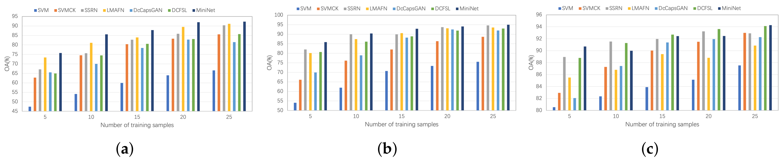
As shown in Figure 12, we further evaluate the classification performance with varied training sample sizes for different comparison algorithms. From Figure 12, we can notice that the classification accuracy gradually improves as the number of training samples increases. It is easy to find that the proposed HyperLiteNet exhibits acceptable satisfactory classification results with different sample sizes.
4. Discussion
4.1. Assessment of the Model Design
According to the experimental results of the different numbers of training epochs (Figure 7c), the HyperLiteNet has the characteristic of fast convergence for different datasets during the training process. In addition, Figure 7a,b confirm that the model complexity and model convergence ability are negatively correlated. The smaller the model, the more difficult it is to find the appropriate parameters. Therefore, the key is to achieve a suitable balance between the efficiency and the model size. Many practical applications only focus on inference costs. Therefore, more training time in exchange for less inference time is feasible for small algorithm models, which can facilitate online leaning in open-scenario circumstances. On the other hand, as can be seen from Table 1, the dynamic convolution on the three datasets improves model performance (from 0.35% to 2.78%) while reducing the number of parameters over 60% and 80% when compared to the SC and MSC. Meanwhile, the dynamic characteristic support the stability of the model on different datasets. This conclusion is further demonstrated through the t-SNE visualization in Figure 8.
4.2. Assessment of the Model Performances
As illustrated in Table 2, Table 3 and Table 4, the HyperLiteNet achieves the highest classification OA—, , and —with gains of , , and over the optimal results in the comparison algorithms on the three experimental datasets under extremely small training sizes. Through an elaborate, lightweight design, the HyperLiteNet reduces the number of parameters by 66%–98% and Flops by 60%–99%, compared to other DL-based comparison algorithms. In terms of training time and testing time, even compared with the fastest LMAFN, the HyperLiteNet still achieves 2.6-times and 4.6-times efficiency improvements. Experiments on three representative datasets indicate that the proposed HyperLiteNet outperforms these state-of-the-art DL-based comparison algorithms with extremely high efficiency and a low number of parameters. However, Figure 9, Figure 10 and Figure 11 show that the classification maps generated by the HyperLiteNet presents oversmoothed results. This phenomenon illustrates that HyperLiteNet achieves efficient classification performance, whereas the lightweight structure of spectral information is apt to result in oversmooth boundaries of classes.
5. Conclusions
At present, small, portable smart devices require low energy consumption and fast response times. This limits the efficiency and size of the DL models. Therefore, it is not advisable to blindly pursue the high complexity of the model in exchange for the improvement of the performance. In this article, an extremely lightweight, non-deep MiniNet model is proposed for HSI classification. The proposed model employs dynamic convolution and a feature interaction module to realize the flexible extraction and interaction of abstract features in different stages, which can further improve the discriminant information of different inputs. Meanwhile, the dual-branch PW and dynamic convolutional structure plays an important role in extracting spectral and spatial features in a hardware-friendly manner through the shallow parallel lightweight structure design, with extremely low numbers of parameters and execution costs.
Author Contributions
Conceptualization, J.W. and R.H.; methodology, J.W. and R.H.; validation, S.G., B.L. and L.L.; investigation, J.W., R.H. and S.G.; writing—original draft preparation, J.W. and R.H.; writing—review and editing, J.W., R.H., Z.P. and B.L. All authors have read and agreed to the published version of the manuscript.
Funding
This work was supported in part by the National Natural Science Foundation of China under grant numbers 61801353 and 61971273, in part by the Key Research and Development Program in Shaanxi Province of China under grant number 2021GY-032, in part by GHfund B under grant number 202107020822, and in part by the Project Supported by the China Postdoctoral Science Foundation funded project under grant number 2018M633474.
Institutional Review Board Statement
Not applicable.
Informed Consent Statement
Not applicable.
Data Availability Statement
Not applicable.
Conflicts of Interest
The authors declare no conflict of interest. The funders had no role in the design of the study; in the collection, analyses, or interpretation of data; in the writing of the manuscript, or in the decision to publish the results.
References
- Xue, Z.; Li, J.; Cheng, L.; Du, P. Spectral–spatial classification of hyperspectral data via morphological component analysis-based image separation. IEEE Trans. Geosci. Remote Sens. 2014, 53, 70–84. [Google Scholar]
- Zhang, L.; Zhang, L.; Tao, D.; Huang, X.; Du, B. Hyperspectral remote sensing image subpixel target detection based on supervised metric learning. IEEE Trans. Geosci. Remote Sens. 2013, 52, 4955–4965. [Google Scholar] [CrossRef]
- Wan, Y.; Hu, X.; Zhong, Y.; Ma, A.; Wei, L.; Zhang, L. Tailings reservoir disaster and environmental monitoring using the UAV-ground hyperspectral joint observation and processing: A case of study in Xinjiang, the belt and road. In Proceedings of the IGARSS 2019-2019 IEEE International Geoscience and Remote Sensing Symposium, Yokohama, Japan, 28 July–2 August 2019; pp. 9713–9716. [Google Scholar]
- Coppin, P.; Jonckheere, I.; Nackaerts, K.; Muys, B.; Lambin, E. Digital change detection methods in ecosystem monitoring: A review. Int. J. Remote Sens. 2004, 25, 1565–1596. [Google Scholar] [CrossRef]
- Hughes, G. On the mean accuracy of statistical pattern recognizers. IEEE Trans. Inf. Theory 1968, 14, 55–63. [Google Scholar] [CrossRef] [Green Version]
- Wang, L.; Li, H.C.; Xue, B.; Chang, C.I. Constrained band subset selection for hyperspectral imagery. IEEE Geosci. Remote Sens. Lett. 2017, 14, 2032–2036. [Google Scholar] [CrossRef]
- Palsson, F.; Sveinsson, J.R.; Ulfarsson, M.O.; Benediktsson, J.A. Model-based fusion of multi-and hyperspectral images using PCA and wavelets. IEEE Trans. Geosci. Remote Sens. 2014, 53, 2652–2663. [Google Scholar] [CrossRef]
- Falco, N.; Benediktsson, J.A.; Bruzzone, L. A study on the effectiveness of different independent component analysis algorithms for hyperspectral image classification. IEEE J. Sel. Top. Appl. Earth Obs. Remote Sens. 2014, 7, 2183–2199. [Google Scholar] [CrossRef]
- Gordon, C. A generalization of the maximum noise fraction transform. IEEE Trans. Geosci. Remote Sens. 2000, 38, 608–610. [Google Scholar] [CrossRef] [Green Version]
- Tarabalka, Y.; Fauvel, M.; Chanussot, J.; Benediktsson, J.A. SVM-and MRF-based method for accurate classification of hyperspectral images. IEEE Geosci. Remote Sens. Lett. 2010, 7, 736–740. [Google Scholar] [CrossRef] [Green Version]
- Song, W.; Li, S.; Kang, X.; Huang, K. Hyperspectral image classification based on KNN sparse representation. In Proceedings of the 2016 IEEE International Geoscience and Remote Sensing Symposium (IGARSS), Beijing, China, 10–15 July 2016; pp. 2411–2414. [Google Scholar]
- Li, J.; Bioucas-Dias, J.M.; Plaza, A. Spectral–spatial hyperspectral image segmentation using subspace multinomial logistic regression and Markov random fields. IEEE Trans. Geosci. Remote Sens. 2011, 50, 809–823. [Google Scholar] [CrossRef]
- Joelsson, S.R.; Benediktsson, J.A.; Sveinsson, J.R. Random forest classifiers for hyperspectral data. In Proceedings of the 2005 IEEE International Geoscience and Remote Sensing Symposium, Seoul, Korea, 29 July 2005; Volume 1, pp. 4–8. [Google Scholar]
- Camps-Valls, G.; Gomez-Chova, L.; Muñoz-Marí, J.; Vila-Francés, J.; Calpe-Maravilla, J. Composite kernels for hyperspectral image classification. IEEE Geosci. Remote Sens. Lett. 2006, 3, 93–97. [Google Scholar] [CrossRef]
- Chen, Y.; Nasrabadi, N.M.; Tran, T.D. Classification for hyperspectral imagery based on sparse representation. In Proceedings of the 2010 2nd Workshop on Hyperspectral Image and Signal Processing: Evolution in Remote Sensing, Reykjavik, Iceland, 14–16 June 2010; pp. 1–4. [Google Scholar]
- Wang, J.; Jiao, L.; Liu, H.; Yang, S.; Liu, F. Hyperspectral image classification by spatial–spectral derivative-aided kernel joint sparse representation. IEEE J. Sel. Top. Appl. Earth Obs. Remote Sens. 2015, 8, 2485–2500. [Google Scholar] [CrossRef]
- Wang, J.; Jiao, L.; Wang, S.; Hou, B.; Liu, F. Adaptive nonlocal spatial–spectral kernel for hyperspectral imagery classification. IEEE J. Sel. Top. Appl. Earth Obs. Remote Sens. 2016, 9, 4086–4101. [Google Scholar] [CrossRef]
- Zhang, L.; Zhang, L.; Du, B. Deep learning for remote sensing data: A technical tutorial on the state of the art. IEEE Geosci. Remote Sens. Mag. 2016, 4, 22–40. [Google Scholar] [CrossRef]
- Chen, Y.; Zhao, X.; Jia, X. Spectral–spatial classification of hyperspectral data based on deep belief network. IEEE J. Sel. Top. Appl. Earth Obs. Remote Sens. 2015, 8, 2381–2392. [Google Scholar] [CrossRef]
- Zhong, Z.; Li, J.; Luo, Z.; Chapman, M. Spectral–spatial residual network for hyperspectral image classification: A 3-D deep learning framework. IEEE Trans. Geosci. Remote Sens. 2017, 56, 847–858. [Google Scholar] [CrossRef]
- Gao, H.; Zhang, Y.; Chen, Z.; Li, C. A Multiscale Dual-Branch Feature Fusion and Attention Network for Hyperspectral Images Classification. IEEE J. Sel. Top. Appl. Earth Obs. Remote Sens. 2021, 14, 8180–8192. [Google Scholar] [CrossRef]
- Li, S.; Luo, X.; Wang, Q.; Li, L.; Yin, J. H2AN: Hierarchical Homogeneity-Attention Network for Hyperspectral Image Classification. IEEE Trans. Geosci. Remote Sens. 2021, 1–16. [Google Scholar] [CrossRef]
- Zhang, T.; Shi, C.; Liao, D.; Wang, L. A Spectral Spatial Attention Fusion with Deformable Convolutional Residual Network for Hyperspectral Image Classification. Remote Sens. 2021, 13, 3590. [Google Scholar] [CrossRef]
- Sabour, S.; Frosst, N.; Hinton, G.E. Dynamic Routing Between Capsules. arXiv 2017, arXiv:1710.09829. [Google Scholar]
- Lei, R.; Zhang, C.; Liu, W.; Zhang, L.; Zhang, X.; Yang, Y.; Huang, J.; Li, Z.; Zhou, Z. Hyperspectral Remote Sensing Image Classification Using Deep Convolutional Capsule Network. IEEE J. Sel. Top. Appl. Earth Obs. Remote Sens. 2021, 14, 8297–8315. [Google Scholar] [CrossRef]
- Wang, J.; Guo, S.; Huang, R.; Li, L.; Zhang, X.; Jiao, L. Dual-Channel Capsule Generation Adversarial Network for Hyperspectral Image Classification. IEEE Trans. Geosci. Remote Sens. 2022, 60, 1–16. [Google Scholar] [CrossRef]
- Bianchini, M.; Scarselli, F. On the complexity of neural network classifiers: A comparison between shallow and deep architectures. IEEE Trans. Neural Netw. Learn. Syst. 2014, 25, 1553–1565. [Google Scholar] [CrossRef] [PubMed]
- Zagoruyko, S.; Komodakis, N. Wide Residual Networks. arXiv 2016, arXiv:1605.07146. [Google Scholar]
- Wu, Z.; Shen, C.; Van Den Hengel, A. Wider or deeper: Revisiting the resnet model for visual recognition. Pattern Recognit. 2019, 90, 119–133. [Google Scholar] [CrossRef] [Green Version]
- Tan, M.; Le, Q. Efficientnet: Rethinking model scaling for convolutional neural networks. In International Conference on Machine Learning; PMLR: Long Beach, CA, USA, 2019; pp. 6105–6114. [Google Scholar]
- Goyal, A.; Bochkovskiy, A.; Deng, J.; Koltun, V. Non-deep Networks. arXiv 2021, arXiv:2110.07641. [Google Scholar]
- Iandola, F.N.; Moskewicz, M.W.; Ashraf, K.; Han, S.; Dally, W.J.; Keutzer, K. SqueezeNet: AlexNet-level accuracy with 50x fewer parameters and <1 MB model size. arXiv 2016, arXiv:1602.07360. [Google Scholar]
- Zhang, X.; Zhou, X.; Lin, M.; Sun, J. Shufflenet: An extremely efficient convolutional neural network for mobile devices. In Proceedings of the IEEE Conference on Computer Vision and Pattern Recognition, Salt Lake City, UT, USA, 18–23 June 2018; pp. 6848–6856. [Google Scholar]
- Howard, A.G.; Zhu, M.; Chen, B.; Kalenichenko, D.; Wang, W.; Weyand, T.; Andreetto, M.; Adam, H. MobileNets: Efficient Convolutional Neural Networks for Mobile Vision Applications. arXiv 2017, arXiv:1704.04861. [Google Scholar]
- Sandler, M.; Howard, A.; Zhu, M.; Zhmoginov, A.; Chen, L.C. Mobilenetv2: Inverted residuals and linear bottlenecks. In Proceedings of the IEEE Conference on Computer Vision and Pattern Recognition, Salt Lake City, UT, USA, 18–23 June 2018; pp. 4510–4520. [Google Scholar]
- Howard, A.; Sandler, M.; Chu, G.; Chen, L.C.; Chen, B.; Tan, M.; Wang, W.; Zhu, Y.; Pang, R.; Vasudevan, V.; et al. Searching for mobilenetv3. In Proceedings of the IEEE/CVF International Conference on Computer Vision, Long Beach, CA, USA, 9 May 2019; pp. 1314–1324. [Google Scholar]
- Han, K.; Wang, Y.; Tian, Q.; Guo, J.; Xu, C.; Xu, C. Ghostnet: More features from cheap operations. In Proceedings of the IEEE/CVF Conference on Computer Vision and Pattern Recognition, Seattle, WA, USA, 13–19 June 2020; pp. 1580–1589. [Google Scholar]
- Zhang, C.; Xu, Y.; Shen, Y. CompConv: A Compact Convolution Module for Efficient Feature Learning. In Proceedings of the IEEE/CVF Conference on Computer Vision and Pattern Recognition, Nashville, TN, USA, 20–25 June 2021; pp. 3012–3021. [Google Scholar]
- Li, D.; Hu, J.; Wang, C.; Li, X.; She, Q.; Zhu, L.; Zhang, T.; Chen, Q. Involution: Inverting the inherence of convolution for visual recognition. In Proceedings of the IEEE/CVF Conference on Computer Vision and Pattern Recognition, Nashville, TN, USA, 10 March 2021; pp. 12321–12330. [Google Scholar]
- Li, Y.; Chen, Y.; Dai, X.; Chen, D.; Liu, M.; Yuan, L.; Liu, Z.; Zhang, L.; Vasconcelos, N. MicroNet: Towards Image Recognition with Extremely Low FLOPs. arXiv 2020, arXiv:2011.12289. [Google Scholar]
- Chen, H.; Wang, Y.; Xu, C.; Shi, B.; Xu, C.; Tian, Q.; Xu, C. AdderNet: Do we really need multiplications in deep learning? In Proceedings of the IEEE/CVF Conference on Computer Vision and Pattern Recognition, Seattle, WA, USA, 13–19 June 2020; pp. 1468–1477. [Google Scholar]
- Ma, N.; Zhang, X.; Zheng, H.T.; Sun, J. Shufflenet v2: Practical guidelines for efficient cnn architecture design. In Proceedings of the European Conference on Computer Vision (ECCV), Munich, Germany, 8–14 September 2018; pp. 116–131. [Google Scholar]
- Zhang, H.; Li, Y.; Jiang, Y.; Wang, P.; Shen, Q.; Shen, C. Hyperspectral classification based on lightweight 3-D-CNN with transfer learning. IEEE Trans. Geosci. Remote Sens. 2019, 57, 5813–5828. [Google Scholar] [CrossRef] [Green Version]
- Jia, S.; Lin, Z.; Xu, M.; Huang, Q.; Zhou, J.; Jia, X.; Li, Q. A lightweight convolutional neural network for hyperspectral image classification. IEEE Trans. Geosci. Remote Sens. 2020, 59, 4150–4163. [Google Scholar] [CrossRef]
- Radosavovic, I.; Kosaraju, R.P.; Girshick, R.; He, K.; Dollár, P. Designing network design spaces. In Proceedings of the IEEE/CVF Conference on Computer Vision and Pattern Recognition, Seattle, WA, USA, 14–19 June 2020; pp. 10428–10436. [Google Scholar]
- Wang, J.; Huang, R.; Guo, S.; Li, L.; Zhu, M.; Yang, S.; Jiao, L. NAS-Guided Lightweight Multiscale Attention Fusion Network for Hyperspectral Image Classification. IEEE Trans. Geosci. Remote Sens. 2021, 59, 8754–8767. [Google Scholar] [CrossRef]
- Cui, B.; Dong, X.M.; Zhan, Q.; Peng, J.; Sun, W. LiteDepthwiseNet: A Lightweight Network for Hyperspectral Image Classification. IEEE Trans. Geosci. Remote Sens. 2022, 60, 5502915. [Google Scholar] [CrossRef]
- Yang, B.; Bender, G.; Le, Q.V.; Ngiam, J. Soft Conditional Computation. arXiv 2019, arXiv:1904.04971. [Google Scholar]
- Zhang, Y.; Zhang, J.; Wang, Q.; Zhong, Z. DyNet: Dynamic Convolution for Accelerating Convolutional Neural Networks. arXiv 2020, arXiv:2004.10694. [Google Scholar]
- Li, Y.; Yuan, L.; Chen, Y.; Wang, P.; Vasconcelos, N. Dynamic Transfer for Multi-Source Domain Adaptation. In Proceedings of the IEEE/CVF Conference on Computer Vision and Pattern Recognition, Nashville, TN, USA, 20–25 June 2021; pp. 10998–11007. [Google Scholar]
- Liu, B.; Yu, X.; Yu, A.; Zhang, P.; Wan, G.; Wang, R. Deep few-shot learning for hyperspectral image classification. IEEE Trans. Geosci. Remote Sens. 2018, 57, 2290–2304. [Google Scholar] [CrossRef]
- Li, S.; Zhang, J.; Ma, W.; Liu, C.H.; Li, W. Dynamic Domain Adaptation for Efficient Inference. In Proceedings of the IEEE/CVF Conference on Computer Vision and Pattern Recognition, Nashville, TN, USA, 10 March 2021; pp. 7832–7841. [Google Scholar]
- Zhong, C.; Zhang, J.; Wu, S.; Zhang, Y. Cross-Scene Deep Transfer Learning With Spectral Feature Adaptation for Hyperspectral Image Classification. IEEE J. Sel. Top. Appl. Earth Obs. Remote Sens. 2020, 13, 2861–2873. [Google Scholar] [CrossRef]
- Hospedales, T.M.; Antoniou, A.; Micaelli, P.; Storkey, A.J. Meta-Learning in Neural Networks: A Survey. arXiv 2020, arXiv:2004.05439. [Google Scholar] [CrossRef]
- Li, Z.; Liu, M.; Chen, Y.; Xu, Y.; Li, W.; Du, Q. Deep Cross-Domain Few-Shot Learning for Hyperspectral Image Classification. IEEE Trans. Geosci. Remote Sens. 2022, 60, 5501618. [Google Scholar] [CrossRef]
- Liang, X.; Zhang, Y.; Zhang, J. Attention Multisource Fusion-Based Deep Few-Shot Learning for Hyperspectral Image Classification. IEEE J. Sel. Top. Appl. Earth Obs. Remote Sens. 2021, 14, 8773–8788. [Google Scholar] [CrossRef]
Figure 1.
(a) The overall flowchart of HyperLiteNet. The five main parts: parallel interconnection module (PIM), pointwise convolution branch (PCB), dynamic convolution branch (DCB), feature interconnection module (FIM), and classification module (CM); (b) pointwise convolution (PW) units with different numbers of convolution kernels; (c) dynamic convolution (DC) unit; (d) fully connected layer (FC); (e) global average pooling (GAP); (f) feature interconnect (FI) structure.

Figure 2.
(a) PW units with the pointwise convolution, BN, and ReLU6. Convert the number of x channels from input channels to 64 (upside); convert the number of input features channels from 64 to 64 (underside). (b) Spectral vectors at a certain point in the l-th layer and the -th layer.
Figure 2.
(a) PW units with the pointwise convolution, BN, and ReLU6. Convert the number of x channels from input channels to 64 (upside); convert the number of input features channels from 64 to 64 (underside). (b) Spectral vectors at a certain point in the l-th layer and the -th layer.

Figure 3.
Adaptive dynamic convolution. (a) Dynamic module composed of the static convolution kernel and the dynamic convolution kernel . realizes subspace routing based on the input adaptive . If is ignored, is equivalent to . (b) Standard dynamic convolution implementation. ⊗ refers to the convolution operation. ⊛ is the input adaptation. The adaptive importance multiplied by the features is equivalent to path selection based on different input samples. (c) DW dynamic convolution implementation. (Both BN and ReLU6 are ignored.)

Figure 4.
IN. (a) False-color image. (b) Ground-truth map. (c) Ground-truth classes.

Figure 5.
UP. (a) False-color image. (b) Ground-truth map. (c) Ground-truth classes.

Figure 6.
SA. (a) False-color image. (b) Ground-truth map. (c) Ground-truth classes.
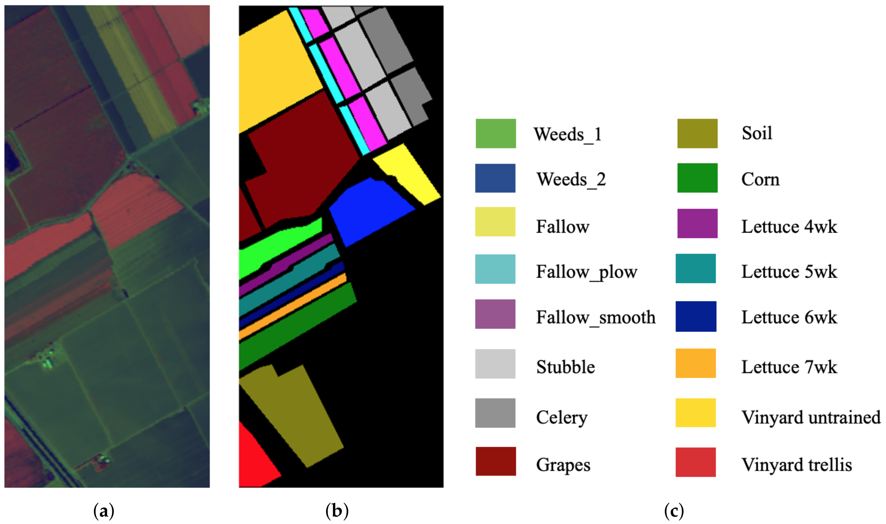
Figure 7.
Effect analysis for the number of convolution kernels, the number of parameters, and the training epoch. (a) OA corresponding to different channel numbers (4000 epochs). (b) Parameters corresponding to different channel numbers. (c) OA corresponding to different training epochs (64 channels).

Figure 8.
2D t-SNE feature visualization for different convolution types on three datasets. The corresponding colored dotted lines are used in the figure to indicate representative differences. (a) IN for DC; (b) IN for SC; (c) IN for MSC; (d) UP for DC; (e) UP for SC; (f) UP for MSC; (g) SA for DC; (h) SA for SC; (i) SA for MSC.

Figure 9.
Classification maps for IN. (a) False-color image; (b) ground-truth map; (c) SVM; (d) SVMCK; (e) SSRN; (f) LMAFN; (g) DcCapsGAN; (h) DCFSL; (i) HyperLiteNet.
Figure 9.
Classification maps for IN. (a) False-color image; (b) ground-truth map; (c) SVM; (d) SVMCK; (e) SSRN; (f) LMAFN; (g) DcCapsGAN; (h) DCFSL; (i) HyperLiteNet.

Figure 10.
Classification maps for UP. (a) False-color image; (b) ground-truth map; (c) SVM; (d) SVMCK; (e) SSRN; (f) LMAFN; (g) DcCapsGAN; (h) DCFSL; (i) HyperLiteNet.
Figure 10.
Classification maps for UP. (a) False-color image; (b) ground-truth map; (c) SVM; (d) SVMCK; (e) SSRN; (f) LMAFN; (g) DcCapsGAN; (h) DCFSL; (i) HyperLiteNet.

Figure 11.
Classification maps for SA. (a) False-color image; (b) ground-truth map; (c) SVM; (d) SVMCK; (e) SSRN; (f) LMAFN; (g) DcCapsGAN; (h) DCFSL; (i) HyperLiteNet.
Figure 11.
Classification maps for SA. (a) False-color image; (b) ground-truth map; (c) SVM; (d) SVMCK; (e) SSRN; (f) LMAFN; (g) DcCapsGAN; (h) DCFSL; (i) HyperLiteNet.

Figure 12.
Overall Accuracy (OA) % with different training samples with 5, 10, 15, 20, and 25 for (a) Indian Pines (IN), (b) Pavia University (UP), and (c) Salinas (SA).
Figure 12.
Overall Accuracy (OA) % with different training samples with 5, 10, 15, 20, and 25 for (a) Indian Pines (IN), (b) Pavia University (UP), and (c) Salinas (SA).


Table 1.
Model performance analysis (OA) and parameters (P) with different convulution types. (1) DC: depthwise separable dynamic convolution; (2) SC: standard convolution; (3) MSC: multi-scale convolution.
Table 1.
Model performance analysis (OA) and parameters (P) with different convulution types. (1) DC: depthwise separable dynamic convolution; (2) SC: standard convolution; (3) MSC: multi-scale convolution.
| Metric | OA | P | OA | P | OA | P | |
|---|---|---|---|---|---|---|---|
| Type | |||||||
| DC | 75.75 ± 3.25 | 59,658 | 85.89 ± 4.60 | 51,939 | 90.70 ± 1.76 | 59,914 | |
| SC | 75.19 ± 3.16 | 153,840 | 83.96 ± 4.88 | 146,121 | 90.35 ± 2.07 | 154,096 | |
| MSC | 75.34 ± 3.62 | 461,616 | 83.11 ± 3.89 | 453,897 | 88.72 ± 4.21 | 461,872 | |
| Dataset | IN | UP | SA | ||||
Table 2.
Classification results (%) on the IN dataset (five labeled samples per class). The best performance values are marked in bold.
Table 2.
Classification results (%) on the IN dataset (five labeled samples per class). The best performance values are marked in bold.
| Class | SVM | SVMCK | SSRN | LMAFN | DcCapsGAN | DCFSL | HyperLiteNet |
|---|---|---|---|---|---|---|---|
| 1 | |||||||
| 2 | |||||||
| 3 | |||||||
| 4 | |||||||
| 5 | |||||||
| 6 | |||||||
| 7 | |||||||
| 8 | |||||||
| 9 | |||||||
| 10 | |||||||
| 11 | |||||||
| 12 | |||||||
| 13 | |||||||
| 14 | |||||||
| 15 | |||||||
| 16 | |||||||
| OA | |||||||
| AA | |||||||
| KP | |||||||
| PA | − | − | 346,784 | 161,451 | 33,521,328 | 4,270,121 | 59,658 |
| Flops (M) | − | − | − | ||||
| Train(s) | − | − | |||||
| Test(s) | − | − |
Table 3.
Classification results (%) on the UP dataset (five labeled samples per class). The best performance values are marked in bold.
Table 3.
Classification results (%) on the UP dataset (five labeled samples per class). The best performance values are marked in bold.
| Class | SVM | SVMCK | SSRN | LMAFN | DcCapsGAN | DCFSL | HyperLiteNet |
|---|---|---|---|---|---|---|---|
| 1 | |||||||
| 2 | |||||||
| 3 | |||||||
| 4 | |||||||
| 5 | |||||||
| 6 | |||||||
| 7 | |||||||
| 8 | |||||||
| 9 | |||||||
| OA | |||||||
| AA | |||||||
| KP | |||||||
| PA | − | − | 199,153 | 153,060 | 21,468,326 | 4,259,294 | 51,939 |
| Flops (M) | − | − | − | ||||
| Train(s) | − | − | |||||
| Test(s) | − | − |
Table 4.
Classification results (%) on the SA dataset (five labeled samples per class). The best performance values are marked in bold.
Table 4.
Classification results (%) on the SA dataset (five labeled samples per class). The best performance values are marked in bold.
| Class | SVM | SVMCK | SSRN | LMAFN | DcCapsGAN | DCFSL | HyperLiteNet |
|---|---|---|---|---|---|---|---|
| 1 | |||||||
| 2 | |||||||
| 3 | |||||||
| 4 | |||||||
| 5 | |||||||
| 6 | |||||||
| 7 | |||||||
| 8 | |||||||
| 9 | |||||||
| 10 | |||||||
| 11 | |||||||
| 12 | |||||||
| 13 | |||||||
| 14 | |||||||
| 15 | |||||||
| 16 | |||||||
| OA | |||||||
| AA | |||||||
| KP | |||||||
| PA | − | − | 352,928 | 161,707 | 34,627,364 | 4,270,521 | 59,914 |
| Flops (M) | − | − | − | ||||
| Train(s) | − | − | |||||
| Test(s) | − | − |
Publisher’s Note: MDPI stays neutral with regard to jurisdictional claims in published maps and institutional affiliations. |
© 2022 by the authors. Licensee MDPI, Basel, Switzerland. This article is an open access article distributed under the terms and conditions of the Creative Commons Attribution (CC BY) license (https://creativecommons.org/licenses/by/4.0/).
Share and Cite
MDPI and ACS Style
Wang, J.; Huang, R.; Guo, S.; Li, L.; Pei, Z.; Liu, B. HyperLiteNet: Extremely Lightweight Non-Deep Parallel Network for Hyperspectral Image Classification. Remote Sens. 2022, 14, 866. https://doi.org/10.3390/rs14040866
AMA Style
Wang J, Huang R, Guo S, Li L, Pei Z, Liu B. HyperLiteNet: Extremely Lightweight Non-Deep Parallel Network for Hyperspectral Image Classification. Remote Sensing. 2022; 14(4):866. https://doi.org/10.3390/rs14040866
Chicago/Turabian StyleWang, Jianing, Runhu Huang, Siying Guo, Linhao Li, Zhao Pei, and Bo Liu. 2022. "HyperLiteNet: Extremely Lightweight Non-Deep Parallel Network for Hyperspectral Image Classification" Remote Sensing 14, no. 4: 866. https://doi.org/10.3390/rs14040866
Note that from the first issue of 2016, this journal uses article numbers instead of page numbers. See further details here.