Abstract
Remotely sensed images with low resolution can be effectively used for the large-area monitoring of vegetation restoration, but are unsuitable for accurate small-area monitoring. This limits researchers’ ability to study the composition of vegetation species and the biodiversity and ecosystem functions after ecological restoration. Therefore, this study uses LiDAR and hyperspectral data, develops a hierarchical classification method for classifying vegetation based on LiDAR technology, decision tree and a random forest classifier, and applies it to the eastern waste dump of the Heidaigou mining area in Inner Mongolia, China, which has been restored for around 15 years, to verify the effectiveness of the method. The results were as follows. (1) The intensity, height, and echo characteristics of LiDAR point cloud data and the spectral, vegetation indices, and texture features of hyperspectral image data effectively reflected the differences in vegetation species composition. (2) Vegetation indices had the highest contribution rate to the classification of vegetation species composition types, followed by height, while spectral data alone had a lower contribution rate. Therefore, it was necessary to screen the features of LiDAR and hyperspectral data before classifying vegetation. (3) The hierarchical classification method effectively distinguished the differences between trees (Populus spp., Pinus tabuliformis, Hippophae sp. (arbor), and Robinia pseudoacacia), shrubs (Amorpha fruticosa, Caragana microphylla + Hippophae sp. (shrub)), and grass species, with classification accuracy of 87.45% and a Kappa coefficient of 0.79, which was nearly 43% higher than an unsupervised classification and 10.7–22.7% higher than other supervised classification methods. In conclusion, the fusion of LiDAR and hyperspectral data can accurately and reliably estimate and classify vegetation structural parameters, and reveal the type, quantity, and diversity of vegetation, thus providing a sufficient basis for the assessment and improvement of vegetation after restoration.
1. Introduction
Ecological restoration refers to the scientific and technological methods used to enhance the resilience of an ecosystem and, supplemented by artificial measures, to gradually restore a damaged ecosystem or allow an ecosystem to develop more naturally [1]. Monitoring vegetation species composition is very important for assessing the effectiveness of ecological restoration and biodiversity management after restoration. Ecological restoration monitoring depends on obtaining timely and accurate statistics. However, vegetation restoration is affected by factors including the soil matrix, plant growth environment, and spatial distribution, so it is difficult to monitor the ecological restoration of vegetation species [2]. Determining the vegetation species composition after ecological restoration is conducive to revealing the type, structure, and spatial distribution of vegetation species, understanding the distribution of vegetation species and their self-sustaining ability, and improving and optimizing their spatial structure [3].
However, difficulties arise in vegetation monitoring due to complex objects, diverse indicators, and the need for covering large regions [4]. Traditional manual surveys use on-site data collection for species identification, but this method is labor- and time-consuming [5], while traditional remote sensing technology typically involves using multispectral images acquired by spaceborne or airborne sensors to collect data and conduct research with fine-scale land classification and land type classification [6,7,8,9]. Chen et al. classified objects after multi-scale segmentation of QuickBird images, and analyzed the accuracy of the C5.0, C4.5, and CART decision tree algorithms in forest object-oriented classification [10]. Zhang et al. integrated Sentinel-1 SAR data and Sentinel-2 multispectral data as data sources, and accurately classified crops in the city of Jining [11]. Based on random forest classifiers, Wang et al. used Landsat multispectral data to identify and classify woodlands in the Mentougou area of Beijing [12]. Li et al. used Ziyuan-3 multispectral satellite data to identify the Beibu Gulf at the junction of Guangdong and Guangzhou, and the mangrove forests in the area were studied [13]. Hill et al. used multi-temporal, multi-spectral data to classify six tree species in British temperate deciduous forests [14]. Madonsela et al. used WorldView-2 multispectral data with multiple phenological periods to classify the savanna in South Africa [15]. However, due to the low resolution of ordinary multispectral images and the small number of image bands, the accuracy of the classification results is often limited [16].
Active remote sensing technology, such as LiDAR, and hyperspectral remote sensing have been applied to ecological restoration monitoring. LiDAR, as a popular type of active remote sensing technology, can achieve the accurate and efficient monitoring and simulation of ecosystems on multiple time and spatial scales [17]. Hyperspectral remote sensing, as a non-destructive, rapid, and real-time monitoring method, employs the high spectral resolution of data, which can reflect the spectral and texture characteristics of different types of vegetation and can be used for the accurate classification of vegetation species composition on a fine scale [18]. Kim et al. used LiDAR data to identify eight broad-leaved trees and seven coniferous trees in the Seattle Botanical Garden in the United States based on the data of the growing season and the dormant season [19]. Ferreira et al. used tropical, seasonal, semi-deciduous forests along the Atlantic coast of Brazil as an example. The research object used airborne hyperspectral data to classify eight tree species in the forest, with overall accuracy of approximately 85% [20]. Alonzo et al. used hyperspectral and LiDAR data to analyze 29 common tree species in Santa Barbara, California, USA. Mapping was carried out using spectrum and crown information, and the classification accuracy at the individual level reached 83.4% [21]. Tao et al. classified five tree species in Gutian Mountain National Nature Reserve based on LiDAR and hyperspectral data [22]. Zhao et al. used hyperspectral and LiDAR data to identify subtropical forest tree species in Shennongjia Nature Reserve using its rich spectral information and tree height information [23]. Yu et al. classified northern forests in Southern Finland and found that the combination of airborne multispectral, LiDAR data, and the random forest algorithm had good performance in tree species classification [24]. However, LiDAR and hyperspectral data are rarely used to study the structure and function, such as carbon sequestration and oxygen release, water conservation, and soil and water conservation, of vegetation after ecological restoration in mining areas.
Therefore, this study attempts to: (1) study the effectiveness of LiDAR point cloud data and hyperspectral image data to reflect the differences among species composition types, and reveal the correlation, information richness, and redundancy among the data extracted from LiDAR and hyperspectral images from the perspective of vegetation; and (2) assess the performance of the hierarchical classification method in classifying vegetation species composition types on four layers—arbors, shrubs, grasses, and bare land.
2. Materials and Methods
2.1. Study Area
The study area is located in the east waste dump of the Heidaigou open-pit mining area in Zhungeer Banner, Ordos City, Inner Mongolia, in Northern China, at 39°43′11′′–39°47′41′′ N, 110°12′53′′–111°20′02′′ E. The dump site is roughly fan-shaped, with a radius of approximately 1.4 km and a slope angle of approximately 30°–40°. The study area was restored from 1993 to 2006; most of the trees and shrubs are less than 20 years old. The accumulated cultivated land area is 235.6 ha, and the study area selected in this study is 20.49 ha, as shown in Figure 1. There is no obvious topographical undulation in the area; the area consists of a large platform.

Figure 1.
Location of study area: (a) location of the study area within the administrative areas of China; (b) location of Ordos City and the study area within Inner Mongolia; (c) a transect (the boundary of red line) of 20.49 ha in the Heidaigou open-pit mine was selected as the study area to collect the LiDAR data, hyperspectral data, and field survey data in this area. The map image cited in the research area is the WorldView-2 image of the Heidaigou area obtained in November 2018.
Before the restoration of vegetation in the study area, the native vegetation had been completely destroyed. In the process of ecological restoration, trees such as Populus spp., Pinus tabuliformis, Amorpha fruticosa, and Robinia pseudoacacia were planted. The planted shrubs in the study area include Amorpha fruticosa, Caragana microphylla, and Hippophae sp. Single species were planted on specific plots. Since 2006, the area has been subjected to no artificial management, and natural succession has begun. In the process of succession, vegetation species are mixed and clustered on plots; some vegetation in the study area died, and these areas degenerated into grassland or bare land.
2.2. Method
2.2.1. Data
The LiDAR data were acquired by a LiAir 220 UAV LiDAR system on 3 August 2020 using a DJI M600 PRO UAV platform (Dajiang Baiwang Technology Co., Ltd., Shenzhen, Guangdong, China) with a HS40P laser sensor. There were two flight zones planned in the flight area, with a total route of 2762 m, a flight altitude of 90 m, and a flight speed of 5 m/s. During LiDAR data acquisition, the horizontal field of view was 360°, the vertical field of view was greater than 20°, and the average point cloud density was 142 /m2.
LiDAR data were pre-processed though track solution, strip splicing, strip redundancy elimination, and point cloud merging [25]. The morphological point cloud filtering method was used to distinguish the ground information in the LiDAR data to obtain the digital elevation model, the first echo characteristic data of the LiDAR was interpolated, and the ordinary kriging interpolation method was selected to generate the surface model. The crop height model (CHM) was expressed as the difference between the digital surface model and the digital elevation model.
Hyperspectral data were acquired by a S185 hyperspectral sensor (Cubert GmbH, Ulm, Germany) mounted on multi-rotor platform. A total of ten routes were planned in this hyperspectral data acquisition scheme, with an observation height of 100 m and a speed of 7.5 m/s. The sensor had a spectral range of 450–998 nm, a spectral resolution of 8 nm, a spectral sampling interval of 4 nm, and a ground resolution that could reach 5 cm.
The pre-processing of collected hyperspectral data is necessary for improving the quality of the hyperspectral images and the efficiency of image processing [26]. The whiteboard data obtained during real-time data acquisition were used to calibrate the sensor; then, atmospheric correction, geometric correction, splicing and cutting of the flight belts, image fusion, and other processing steps were completed [27]. In this study area, 1780 images were collected in a single band, while the mosaic of single-band images was operated through the Agisoft photoscan platform (www.agisoft.com, accessed on 12 November 2020). During the data pre-processing, radiometric calibration, atmospheric correction, geometric correction, and image band synthesis were all realized with the help of the ENVI platform (Research Systems, Inc., Boulder, CO, USA).
LiDAR data were used to extract the intensity, height, and echo features of vegetation, while the hyperspectral image data were used to extract the vegetation spectrum, vegetation index, and texture features. Statistical analysis and correlation analysis by OriginLab (www.originlab.com, accessed on 4 March 2021) and IBM SPSS Statistics (www.ibm.com, accessed on 9 March 2021) were used to explore the relationships between vegetation features. The resampling tool of the ENVI platform (Research Systems, Inc., Boulder, CO, USA) was used to convert the resolution of the LiDAR data and hyperspectral data to 1 × 1 m [28,29].
Field survey data were collected simultaneously with the collection of UAV LiDAR and hyperspectral image data. Using random and typical sampling techniques, 10 m × 10 m quadrats were used to sample the vegetation. A total of 52 quadrats were investigated, including recording the vegetation type, canopy coverage, and dominant vegetation in each quadrat, as well as the tree height, diameter at breast height of trees, and the leaf area index of the dominant vegetation. A 1 × 1 m small quadrat was designated at the center of each large quadrat for the measurement of vegetation coverage and gap fraction by the needling method. In addition, 140 sampling points were established mainly for investigating the vegetation type, leaf area, and tree height index of these sampling points; location information for these sampling points was recorded.
2.2.2. Overall Technical Process
Figure 2 shows the hierarchical classification flow chart of vegetation species composition. After performing feature analysis on LiDAR and hyperspectral images, using the results of feature analysis as empirical knowledge, a hierarchical classification inversion method was developed, combined with a decision tree and random forest algorithm, to construct a vegetation species composition type inversion model. The vegetation index was used to extract the bare land area in the first layer, the bare land area overlapping with the herb area was removed from the height, and then the grassland area was extracted in the second layer. The images of the study area were classified using the single tree crown extraction results, and the trees of Populus spp., Pinus tabuliformis, Hippophae sp. (arbor), and Robinia pseudoacacia were classified in the third layer. Finally, the shrub areas of Caragana microphylla + Hippophae sp. (shrub) and Amorpha fruticosa were extracted from the fourth layer based on the vegetation spectrum.
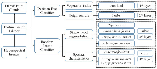
Figure 2.
Hierarchical classification flow chart of vegetation species composition.
After obtaining reliable classification results of vegetation species composition, 15 × 15 m fishing nets were used to divide the study area; then, the number of vegetation species compositions was counted, excluding bare land, using ArcGIS (Research Systems, Inc., RedLands, CA, USA) [30]; the number of vegetation species in each grid was obtained as the number of vegetation species compositions.
2.2.3. Extraction of Feature Factors
- Height
An airborne LiDAR system can be used to obtain three-dimensional coordinate information of a target and extract the height feature of vegetation by processing the point cloud, which is also one of the important parameters related to vegetation structure [31]. A morphological point cloud filtering method was used to distinguish the ground information within the LiDAR data. Based on this elevation model, the point cloud elevation value was subtracted from the value in the corresponding digital elevation model, so that the influence of topographical factors on the estimation of vegetation structure parameters was reduced, allowing the height feature of LiDAR to be extracted.
In this study, the following eight height features were selected: height percentile of 95% (HP95), maximum height (MaxH), minimum height (MinH), mean height (MeaH), median height (MedH), standard deviation of height (SDH), root mean square of height (RMSH), and coefficient of variation (CVH).
- 2.
- Intensity
The LiDAR intensity quantitatively describes the backscattering of an object. Intensity is a measurement index (collected for each point) that reflects the intensity of the LiDAR pulse echo generated at a certain point. The intensity feature can be used to classify the LiDAR points, and the different features can be distinguished by the intensity signal. Studies have shown that the influence of leaves, branch directions, terrain changes, and laser path length can cause differences in the intensity of LiDAR in forest areas [32].
The following seven features of LiDAR intensity were selected: intensity percentile of 99% (IP99), maximum intensity (MaxI), minimum intensity (MinI), mean intensity (MeaI), median intensity (MedI), standard deviation of intensity (SDI), and coefficient of variation of intensity (CVI).
- 3.
- Echo
The echo feature of LiDAR point cloud data is an important feature that can be used to express the structural parameters of vegetation. A laser pulse emitted may return to the LiDAR sensor in the form of one or more echoes. The first laser pulse returned is the most important echo, and it will be associated with the highest elements on the Earth’s surface (such as treetops). When the first echo represents the ground, the LiDAR system will only detect one echo. Multiple echoes can detect the height of multiple objects within the laser foot point where the laser pulse is emitted. The middle echo usually corresponds to the vegetation structure, and the last echo is related to the exposed terrain model [33].
The laser sensor used for data acquisition in this study could receive two echoes. There was often no obvious difference between the first echo number (Return1) and the second echo number (Return2). Therefore, we defined the ratio of the first echo to the second echo as the third characteristic factor (Return1/2), and observed the difference between the ratio of the two echoes in dense and sparse vegetation areas in the study area.
- 4.
- Spectrum
Different types of vegetation and non-vegetated areas have different absorption and reflection spectral characteristics in different bands [34]. As shown in Figure 3, in the visible band, chlorophyll is the most important factor that dominates the spectral response of plants. In the near-infrared band of the spectrum, the spectral features of vegetation are mainly controlled by the internal structure of plant leaves. Between the visible light band and the near-infrared band, i.e., in the range of 700–998 nm, most of the energy is reflected, a small part of the energy is absorbed, and the rest of the energy is completely transmitted, forming a “red edge” phenomenon, which is the most obvious feature of the plant curve [35].
According to the results of the field survey, the study area was divided into seven vegetation species composition types and the bare land was used for comparison. The region of interest (ROI) data of each object were collected, and the spectral sample data of 138 bands were outputted to form a spectral curve [36].
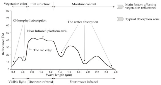
Figure 3.
Schematic diagram of plant spectral curve [37].
Figure 3.
Schematic diagram of plant spectral curve [37].

- 5.
- Vegetation index
Hyperspectral images are easily affected by the environment, atmosphere, and the phenomenon of “different objects with the same spectrum” when researchers attempt to identify different species composition types. The vegetation spectrum shows a complex mixed reaction to vegetation, environmental effects, brightness, soil color, and humidity, which are affected by the spatial–temporal changes in the atmospheric environment. The vegetation index mainly reflects the difference between the reflection of vegetation in the visible light and near-infrared band as well as the soil background [38]. Under certain conditions, each vegetation index can be used to quantitatively explain the growth status of vegetation, and can qualitatively and quantitatively detect and evaluate the vegetation coverage and its growth [39]. Therefore, this study selected the following 33 vegetation indices, listed in Table 1, to study.

Table 1.
Calculation formulae of vegetation indices.
- 6.
- Texture
Texture is an important type of structural information related to the spatial distribution of ground objects. By measuring the difference between pixels and their surrounding spatial neighborhood, texture can be used as a sufficient auxiliary basis for solving the problem of “different spectra of the same object” or “different objects with the same spectrum”, and can make up for a deficiency of spectral features in hyperspectral remote sensing image classification to a certain extent. Texture has three features: scale, region, and regularity. In this study, eight quadratic statistics, listed in Table 2, were used as texture feature parameters to extract the textural features of images.
Table 2.
Calculation formulae of texture indices.
Through combination with the spectral curve images of different vegetation species composition types, it can be seen that the difference in reflectance in the visible light band from different kinds of plants is small. We can consider that the three bands of green, red, and near-infrared can form a pseudo-color image synthesis band that can be used to analyze and extract texture features:
The first two bands of the transformed hyperspectral data are separated by a minimal amount of noise; the pseudo-color bands composed of the green, red, and near-infrared bands were named B1, B2, and B3 when used in the subsequent texture calculations. The central wavelengths of the B1 and B2 bands were 784 nm and 806 nm, respectively. Using a 3 × 3 pixel window, based on the first- and second-order probability statistics, respectively, a gray level co-occurrence matrix of synthetic band images was calculated, and the vegetation texture features were extracted. The naming rules of texture feature factors were defined as: band–texture index–probability statistics order.
- 7.
- Single tree segmentation
The watershed segmentation algorithm is a kind of image segmentation algorithm, which is based on the mathematical morphology principle of topology theory. This method is fast and accurate, so it is widely used in image segmentation [67]. Through a watershed algorithm, a single tree can be segmented, and the position and crown width of a single tree can be obtained. Each pixel in a canopy height model as assigned with an elevation value, resulting in a continuous surface with scattered peaks and valleys. Therefore, the peak point of a continuous surface was defined as the highest point of a single tree. In addition, watershed segmentation can better identify edges, which is more suitable for the high-resolution remote sensing images extracted in this study.
2.2.4. Decision Tree Classifier
A decision tree is a tree data structure based on root, intermediate, and leaf nodes [68]. According to the experimental samples, the decision tree classifier determined the appropriate discriminant function; next, the branches of the tree were constructed according to the obtained functions, and then sub-branches were constructed according to the needs of each branch to form the final decision tree for herb and bare land extraction [69]. Based on empirical knowledge, vegetation and non-vegetation are quite different in remote sensing images, and have strong discrimination characteristics. The study area is a mine dump, and the only bare land types are found in non-vegetation regions.
According to the extraction results of the vegetation index, the vegetation index sensitive to herbs and bare land was selected, and the classification rules of vegetated areas and bare land area were defined. According to the numerical distribution of different vegetation species compositions in the vegetation index, the bare land area could be extracted in the first layer. In addition, obvious differences in height features existed among herbs, trees, and shrubs. Therefore, the classification rules of herbs were summarized by analyzing the numerical distribution of height features between herbs and other vegetation species’ compositions; however, overlapping layers may exist between bare land and herbs in the height layer. Therefore, it is necessary to consider removing bare land and extracting the herb layer in the second layer in the herb layer obtained by height features.
2.2.5. Random Forest Classifier
A random forest algorithm is an ensemble learning algorithm based on a classification regression decision tree. By sampling from training samples using the RF Bootstrap Resampling method, a certain number of samples are repeatedly extracted from the training sample set N, and a new training set of n samples is generated; each sample generates a classification tree, and the n classification trees form a random forest. When a certain number of decision trees are produced, the test samples can be used to test the classification effect of each number, so as to vote for the best classification result [70].
Before using the RF algorithm for classification, the factors of each feature were sorted by random forest; the factors that were more important for the inversion of vegetation species composition types in each feature were screened out [71]. After the classification features were determined, n training sets were obtained by using the autonomous sampling method. Each training set needed to be trained to generate a corresponding decision tree model; next, parameters such as the number of base estimators (n_estimators), the maximum depth (max_depth), the minimum sample size (min_samples_split), and the maximum feature number (max_features) of the random forest were tested [72].
After extracting herbs and bare land, the random forest algorithm was used to invert the tree and shrub species composition types. At first, the image of the study area was classified using the results of canopy extraction and single wood segmentation, i.e., the third layer extracted trees. Finally, the shrubs were classified on the fourth layer.
2.3. Accuracy Verification and Comparison
2.3.1. Accuracy Verification
In this study, two methods were used to evaluate the classification accuracy, namely the overall classification accuracy method and the Kappa coefficient method. Overall classification accuracy is defined as the percentage of the number of correctly classified data points (n) and the number of all points in the inspection area (N) using Equation (2):
A Kappa coefficient (k) is used to test data consistency, which can indirectly reflect classification accuracy, as shown in Equations (3) to (5).
where P0 represents the observed consistency, Pe represents the expected consistency, Xii represents the diagonal element value of the confusion matrix, xi represents the sum of observed values in row I, xj represents the sum of observed values in column j, r represents the total number of rows/columns, and N represents the total number of samples. The value range of k is [−1, 1], and the closer k is to 1, the higher the consistency of the data sets and the better the classification.
In this study, 70% of the survey samples of vegetation species composition were selected as training data, and 30% of the samples were used for verification. The hierarchical classification algorithm of vegetation species composition was established by using a decision tree classifier and random forest classifier.
2.3.2. Accuracy Comparison
With the help of the ENVI platform (Research Systems, Inc., Boulder, CO, USA), the vegetation species composition types in the study area were classified by using the IsoData method in an unsupervised classification, along with the maximum likelihood method, a support vector machine, and a random forest method in supervised classification. The IsoData algorithm first selected the initial class average, and, in the multidimensional data space, divided the pixel classes according to the shortest distance from the center of the training sample class. The maximum likelihood classification rule was used to construct a discriminate classification function by taking the distribution of satellite remote sensing multi-band data as having a multidimensional normal distribution. The support vector machine method can automatically find those support vectors that can best distinguish the classification, and thus construct a classifier, which can maximize the interval between classes, thus having better generalization and higher classification accuracy.
3. Results
3.1. Feature Factor Library
3.1.1. Height
The HP95 reflects the distribution of the true height of vegetation, while the standard deviation of height reflects the difference in height distribution of various vegetation species compositions, and the difference in height distribution of trees is relatively large [31]. Maximum height and mean height feature factors show the same vegetation height arrangement order as a 95% height percentile. Figure 4 shows that in the ordering of median height and standard deviation of height, all vegetation species compositions show the same order. The height variation coefficient can reflect the degree of dispersion in the height distribution of different vegetation species compositions, with Populus spp. having the highest dispersion degree, followed by Caragana microphylla + Hippophae sp. (shrub), while Robinia pseudoacacia and Amorpha fruticosa have the most concentrated height distribution.
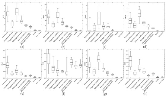
Figure 4.
Height distribution (in meters) of eight types of vegetation species composition: (a) height percentile of 95% (HP95); (b) maximum height (MaxH); (c) minimum height (MinH); (d) mean height (MeaH); (e) median height (MedH); (f) coefficient of variation (CVH); (g) root mean square of height (RMSH); (h) standard deviation of height (SDH).
Table 3 shows the order of vegetation height in the study area was Hippophae sp. (arbor) > Populus spp. > Robinia pseudoacacia > Pinus tabuliformis > Amorpha fruticosa > Caragana microphylla + Hippophae sp. (shrub) > herbs.
Table 3.
The heights of trees, shrubs, herbs, and bare land with maximum, minimum, median, and standard deviation values.
3.1.2. Intensity
The intensity percentile of 99%, maximum intensity, mean intensity, median intensity, and standard deviation of intensity of different vegetation species compositions are shown in Figure 5.
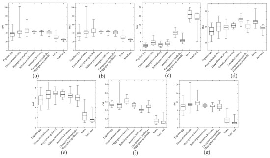
Figure 5.
Intensity distribution of eight types of vegetation species composition: (a) intensity percentile of 95% (IP99); (b) maximum intensity (MaxI); (c) minimum intensity (MinI); (d) mean intensity (MeaI); (e) median intensity (MedI); (f) coefficient of variation of intensity (CVI); (g) standard deviation of intensity (SDI).
The LiDAR intensity values for Populus spp. were the lowest among the tree and shrub species compositions, among which the intensities of herbs and bare land were lower than those of Populus spp., while that of bare land was lower than that of herbs. In the study area, Populus spp., herbs, and bare land species composition were sparsely vegetated areas, and other vegetation canopies were relatively dense, which indicates that there is a certain relationship between the intensity feature and whether the vegetation is dense [32]. The variation coefficient of intensity of Populus spp. was only lower than that of Hippophae sp. The minimum intensity characteristics showed that the order of intensity of the vegetation species compositions was herbs > bare land > shrubs > trees.
3.1.3. Echo
As shown in Figure 6, in contrast to its intensity, Populus spp. showed an obvious advantage in echo characteristics, which were the highest in both the first and second echoes. However, the ratio of the two echoes showed that the first echo number of Populus spp. was lower than the second echo number. According to the investigation, the obvious differences between Populus spp. and other trees and shrubs in the study area were its canopy structure and spatial planting density, which demonstrated that the spatial structure of the vegetation canopy had an important influence on its echo characteristics [33].

Figure 6.
Echo distribution of eight types of vegetation species composition: (a) the first echo; (b) the second echo; (c) the ratio of the first echo to the second echo.
The ratio of the two echoes between herbs and bare land was generally small, and the distribution was concentrated in the areas with a value of 1, which indicated that the first and last echo numbers in herbs and bare land areas were basically equal.
3.1.4. Spectrum
The spectral curves of plants extracted from hyperspectral images were consistent with the measured spectral images in the field, as shown in Figure 7. Because of the different amounts of chlorophyll content of different vegetation species, the reflectance of herbs was higher, and the spectrum of bare land was obviously different from that of plants [34,35].
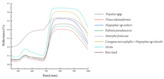
Figure 7.
Spectral curves of seven types of vegetation species composition and bare land.
The results showed that, in the range of 500–700 nm, the spectral reflectance between the bare land and various vegetation species compositions had extreme variations. The phenomenon of “different objects with the same spectrum” appeared in the spectral range of 700–750 nm, so that it was not convenient to distinguish vegetation species composition. In the range of 750–900 nm, each vegetation species composition showed a different level of spectral reflectance. The spectral reflectance of the Amorpha fruticosa and Hippophae sp. (arbor) was very similar, but they could be distinguished at 900–1000 nm. The spectral curve of bare land and the reflectivity of Caragana microphylla + Hippophae sp. (shrub) changed obviously near 950 nm. This may cause errors in species composition classification. Therefore, the spectral range of 750–950 nm was selected to identify and separate different vegetation species compositions. In this band, each vegetation species composition showed different characteristics, and their reflectivity was quite different.
3.1.5. Vegetation Index
Figure 8 shows that the sensitivity of the vegetation index to soil was low. Specifically, CHIgreen, CHIred_edge, DD, GM, mSR750, PBI, RVI, SPI, TVI, and others each formed a peak, which was sensitive to vegetation and soil.
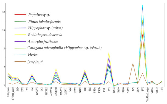
Figure 8.
Vegetation indices of eight types of vegetation species composition.
Among these indicies, CHIgreen, CHIred_edge, GM, mSR750, PBI, and RVI were the most sensitive to Robinia pseudoacacia, the SPI was the most sensitive to soil, and the TVI was more sensitive to vegetation, with herbs being the most important, which can allow vegetation to be distinguished from bare land [38,39]. Among the vegetation indices sensitive to vegetation, the characteristic values of dense Robinia pseudoacacia and Amorpha fruticosa were generally higher, while the characteristic values of herbs were lower.
3.1.6. Texture
Figure 9 shows the differences in the texture of the eight types of vegetation species composition. Contrast represents the complexity of texture, while image heterogeneity is described by dissimilarity [67]. The two bands were separated by a minimal amount of noise, which can reflect the contrast and dissimilarity of vegetation. The vegetation textures in the two bands obtained by the minimal noise separation show the same changing trend, among which the differences in three texture indices, namely second-order contrast, dissimilarity, and mean, are relatively significant. Among these, the difference in second-order contrast in the B2 band was the most obvious, while the differences in second-order mean and second-order variance in the B2 band were more significant. The significance of the second-order correlation and entropy texture index in the B1 and B2 bands followed closely.

Figure 9.
Textures of eight types of vegetation species composition.
Figure 9 shows that little difference existed between the second moment and the first variance texture of vegetation species compositions. In the pseudo-color band, the difference in texture parameters of vegetation species compositions was relatively small, and the median of the second-order mean texture factor of herbaceous vegetation and bare land was much higher than that of other vegetation species compositions. Meanwhile, the first-order variance texture factor was far lower than that of other vegetation species compositions. The second-order mean and second-order contrast texture of the three bands of each vegetation species composition were higher, which indicates that the vegetation had a higher degree of regularity, which is consistent with the characteristics of the reconstructed vegetation in the mining area.
3.2. Decision Tree Classifier
Before the decision tree classifier was used for classification, the classifier parameters were limited to improve the operational efficiency. The result of parameter adjustment is shown in Figure 10.
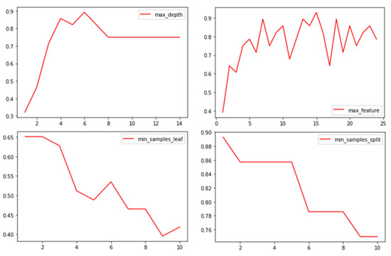
Figure 10.
Parameter adjustments of the decision tree classification algorithm; the x-axis is the number of input feature factors, and the y-axis is the classification efficiency of the classifier after inputting feature factors.
According to the vegetation index results, the vegetation index that was more sensitive to vegetation and soil was selected to define the classification rules of herbs and bare land, as shown in Table 4.
Table 4.
Extraction of vegetation indices of grassland and bare land by a decision tree classifier.
As shown in Table 4, when TVI < 15 or SPI > 1.25, bare land could be well separated. Then, based on the distribution of vegetation height characteristics, the HP95 < 0.85 was selected to extract bare land and herbs, the decision rule of separating bare land and herbaceous areas was established as shown in Figure 11. The difference between bare land and other vegetation groups was defined by setting thresholds of triangle vegetation index (TVI), standardized precipitation index (SPI), modified soil-adjusted vegetation index (MSAVI), Gitelson and Merzlyak index (GM), and ratio vegetation index (RVI); the difference between herbs and other groups was defined by the HP95 height characteristic index, and a filtering window was established to extract bare land and herbaceous areas.

Figure 11.
The decision tree classifier for classifying bare land, herbs, and other species compositions.
3.3. Random Forest Classifier
Figure 12 shows the ranking results of feature importance after each feature was input into the random classifier alone. There were feature factors in each feature that contributed little to the classification results. Therefore, the top 10 factors in the ranking of feature importance were selected for final classification.
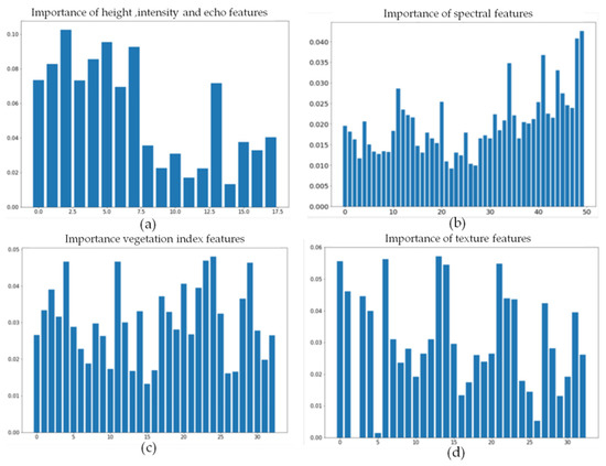
Figure 12.
Importance ranking of four feature factors: (a) height, intensity, and echo; (b) spectrum; (c) vegetation index; (d) texture. The x-axis is the number of feature factors, and the y-axis is the importance of the input feature factors.
The selected factors in each feature are shown in Table 5. Among the following three features, intensity, height, and echo, the height features were the most important. Among the spectral features of vegetation, the selected important feature factors were located in the 834–950 nm bands, which indicate that the near-infrared band plays an important role in identifying the types of vegetation species compositions. Among vegetation indices, the ratio vegetation index R800 and difference vegetation index R600 are of higher importance. Among texture features, vegetation mean and correlation texture are more effective for the inversion of vegetation species composition types.
Table 5.
Importance ranking of the feature factors.
In addition, the performance of each individual feature in the random forest classifier was tested by the verification set. The inversion accuracy of the intensity, height, and echo features extracted from the point cloud data and texture features were higher at 0.7, while the inversion accuracy of the vegetation spectral features alone was the lowest at only 0.45. Therefore, we considered the comprehensive application of each feature, carried out the inversion of vegetation species composition types, and improved the accuracy of the inversion results.
Figure 13 shows the order of importance for each feature factor of vegetation species composition. The vegetation index feature was found to play an important role in the inversion of vegetation species composition types in this study area, followed by the height, texture, and spectral features.
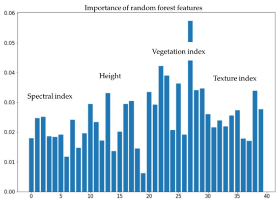
Figure 13.
The importance of features in the estimation of different vegetation species compositions. The x-axis is the number of features, and the y-axis is the importance of the features.
Before the random forest classifier was used for classification, the classifier parameters were limited to improve the operational efficiency as shown in Figure 14. Taking the tree classifier as an example, the number of optimal base classifiers was 61, the maximum depth of trees in random forest was seven, the maximum number of features was 16, and the minimum sample size was two. Shrubs were used and the same command was performed.
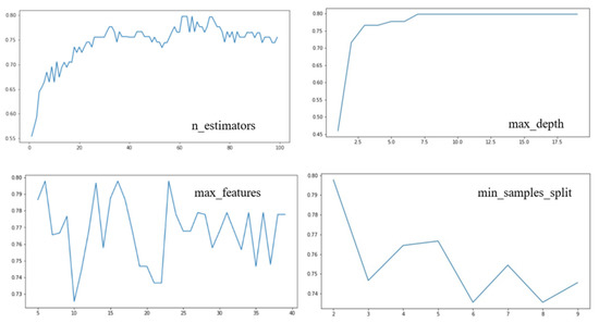
Figure 14.
Parameter adjustments of the random forest classification algorithm; the x-axis is the number of input feature factors, and the y-axis is the classification efficiency of the classifier after inputting feature factors.
The results of random forest classifier construction are shown in Figure 15; the difference between trees and other vegetation species compositions was defined by the threshold values of vegetation index, height, and spectral, and four kinds of tree groups were identified. Then, the difference between shrub areas and other groups was defined by the spectral, and a filter window was established to extract shrubs.
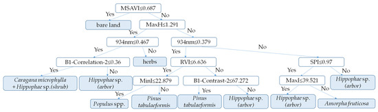
Figure 15.
The random forest classifier for classifying trees and shrubs.
3.4. Classification Results
The reconstructed vegetation in the study area is all artificially planted. Figure 16 show that the reconstructed vegetation has a relatively obvious spatial structure. The vegetation of the open-pit mine dumps undergoes natural succession. Under different vegetation species compositions, the vegetation clusters show unique structural succession characteristics.
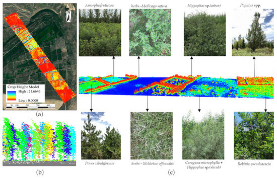
Figure 16.
(a) Canopy heights of trees, shrubs, herbs, and bare land in study area; (b) cross-sectional view of single tree segmentation result; (c) three-dimensional models of different vegetation species compositions.
Based on LiDAR and hyperspectral data, the height, intensity, echo, spectral, vegetation index, and texture features of vegetation were extracted, and the classification results of the vegetation species compositions are shown in Figure 17.

Figure 17.
Classification results: (a) the first layer of bare land; (b) the second layer of herbs; (c) the third layer of trees—Populus spp., Pinus tabuliformis, Hippophae sp. (arbor), and Robinia pseudoacacia; (d) the fourth layer of shrubs—Caragana microphylla + Hippophae sp. (shrub) and Amorpha fruticosa.
As shown in Figure 17, the northern part of the study area consists of a large area of Populus spp., herbs, and bare land, among which there is a larger area of Hippophae sp. (arbor). The vegetation species composition patterns in the central and northern regions include mixed areas of Caragana microphylla + Hippophae sp. (shrub) and Populus spp., as well as mixed areas of Hippophae sp. (arbor), Caragana microphylla + Hippophae sp. (shrub), and herbaceous species compositions. In addition, there is a larger area of Robinia pseudoacacia; in the middle of the study area, the vegetation species included Robinia pseudoacacia, Hippophae sp., Amorpha fruticosa, and Populus spp. This area mainly consisted of Hippophae sp. (arbor), Amorpha fruticosa, Caragana microphylla + Hippophae sp. (shrub), and herbaceous species composition patterns, as well as large areas of grassland and bare land, with a small amount of mixed planting of Hippophae sp. (arbor). Amorpha fruticosa was planted in most areas in the central and southern parts of the study area, Hippophae sp. (arbor) was mixed-planted around the Amorpha fruticosa clusters, and Populus spp., Caragana microphylla + Hippophae sp. (shrub), and Pinus tabuliformis were mixed-planted in some areas. The vast majority of the southern part of the study area was grassland, with a small amount of Hippophae sp. (arbor) and Pinus tabuliformis mixed-planted in it and with a few Populus spp. scattered sporadically.
3.5. Accuracy
3.5.1. Accuracy of Other Classification Methods
Identification and classification experiments for vegetation species compositions in the region were carried out. Figure 18 shows the classification results of vegetation species composition types obtained after using other classification methods; Table 6 provides the accuracy evaluation results of each classification method.

Figure 18.
The results of vegetation species composition types using different classification methods: (a) IsoData unsupervised classification; (b) maximum likelihood supervised classification; (c) support vector machine classification; (d) direct random forest classification.
Table 6.
Accuracy of the classification of vegetation species compositions.
The IsoData unsupervised classification method had the lowest classification accuracy and could only identify part of the region with vegetation; however, most of the areas could not be correctly identified. The similar spectral curves in the vegetation species compositions seriously interfered with the classification results, making it impossible to identify the types of fine-scale vegetation species compositions present in the study area. As for the maximum likelihood method, Hippophae sp. and Robinia pseudoacacia were difficult to distinguish; support vector machines would easy confuse poplars at the edges of roads, and the random forest rules could not completely extract trees, so there were many broken patches in the tree areas, and the classification results were inaccurate. It can be seen that the general supervised classification method, taking the maximum likelihood method as an example, allowed the researchers to identify more types of vegetation species compositions than the unsupervised classification method, but the identification results were incomplete and inaccurate.
3.5.2. Accuracy of the Hierarchical Classification Method
In the process of extracting the number of vegetation species compositions, a hierarchical classification method was developed. The hierarchical classification method extracts the tree region based on expert knowledge and single tree segmentation. In addition, the fine-scale classification of vegetation species compositions was realized by combining a decision tree and random forest algorithm. The hierarchical classification method was used based on expert knowledge and tree regions extracted by single tree segmentation; the overall classification accuracy was 87.45%, and the consistency of the data sets was the highest, with a Kappa coefficient reaching 0.79. The overall user accuracy improved by nearly 43% when compared with unsupervised classification methods, and the accuracy improved by 10.7–22.7% when compared with other supervised classification methods. This indicates that the hierarchical classification method has certain advantages in vegetation species composition identification.
4. Discussion
4.1. Performance of Different Classification Methods
When faced with different remote sensing data and different feature variables, IsoData, support vector machine, the maximum likelihood method, and random forest classifiers show differences in classification performance [73,74,75,76]. Gu et al. compared land use information extraction models such as support vector machines, BP neural networks, and random forests, and they found that the random forest classification method had the highest accuracy [77]. Chen et al. studied the classification of land use in industrial and mining reclamation areas and found that the execution time and accuracy were better than support vector machine under the same characteristic variables [78]. Yang et al. used random forests and support vector machines to map tree species in the Northern Alberta forest region, and random forests outperformed support vector machine classifiers [79]. Zhao et al. used the maximum likelihood method, support vector machine, and random forest to classify the dominant tree species of shelterbelts [80]. Yang et al. built a random forest classification model that integrated 24 variables, including spectral features, vegetation features, terrain features, and texture features, and combined it with support vector machine, K-nearest neighbor, and maximum likelihood classification methods [81]. Li et al. used Sentinel-1 and Sentinel-2A satellite images and a digital elevation model as data sources to combine the random forest and recursive feature elimination algorithm, and the classification accuracy was better than the support vector machine algorithm and K-nearest neighbor algorithm with the same features [82].
These studies show that there are great differences between the actual data of different research objects and places, and that different numbers of classified species will also affect the classification results. In our study, the IsoData unsupervised classification method could only identify some areas with vegetation, the maximum likelihood method was unable to distinguish between Hippophae sp. (shrub) and Robinia pseudoacacia, the support vector machine confused Populus spp. at the edge of the road, and the random forest rule could not fully extract the trees. Therefore, it is impossible to judge the quality of a classification algorithm based on the classification accuracy alone. In addition, a specific algorithm has the best expressive force when it utilizes the data that best conform to its operational principle format [83,84,85]. With the increasing requirement of classification accuracy, the multiple-classifier systems algorithm is developing gradually. Compared with a single classification algorithm, multiple-classifier systems can integrate the advantages of multiple classification algorithms and select the appropriate combination of algorithms to improve the accuracy of the classification results [86].
4.2. Spatial Analysis of Vegetation Species Composition Types
Vegetation species composition number is defined as the number of different vegetation species, including trees, shrubs, and herbs, in a certain grid with a resolution of 15 m. This parameter can reflect the spatial distribution of vegetation species abundance.
As shown in Figure 19, in the study area, the vegetation species composition in the following three areas had more vegetation species: (1) the intersection of Caragana microphylla + Hippophae sp. (shrub) and Populus spp.; (2) the mixed area of Robinia pseudoacacia, Hippophae sp. (arbor), and Caragana microphylla + Hippophae sp. (shrub) in the middle and northern parts of the study area, and (3) the junction of Amorpha fruticosa and Pinus tabuliformis in the middle and southern parts of the study area. In the middle and southern parts of the study area, the mixed area of Robinia pseudoacacia, Hippophae sp. (arbor), Amorpha fruticosa, and herbs had good diversity and reasonable vegetation species composition.

Figure 19.
Estimation results of (a) fine identification and classification of seven vegetation species compositions in the study area: Populus, Pinus tabuliformis, Sea buckthorn (arbor), Robinia pseudoacacia, Amorpha fruticosa, Caragana microphylla + Sea buckthorn (shrub), herbs, and bare land; (b) vegetation species composition number; the numbers 1 to 7 represent the number of vegetation species compositions in a specific patch.
Following natural regeneration, competition, species replacement, and human intervention with appropriate intensity, some areas will show vegetation distribution characteristics different from those in the planning period. Vegetation species composition will increase as the process of succession occurs [87]. In the process of succession, plants with a weak competitive ability gradually die out, and the number of vegetation species will decline to a certain extent [88]. It can be seen from the estimation results of vegetation species composition that the vegetation is relatively sparsely distributed, with little competition in the edge habitat, where the vegetation species composition meets roads in the study area. Among the areas with a single vegetation species composition, the areas with a low number of vegetation species composition types included bare land and herbs, some of which were originally planned to be individual Acacia or Prunus humilis plantations; however, many of these areas have degenerated into areas with only herbs or into bare land. The mixed areas of multiple types of vegetation species composition, with broad-leaved trees such as Populus spp., Robinia pseudoacacia, and Amorpha fruticosa, have more types of vegetation species, representing mixed clusters of plant species.
Therefore, a better species composition of vegetation would be a mixture of trees, shrubs, and herbs, which can achieve the effects of reasonable spatial distribution as well as the full and effective use of ecological resources; this species composition will form an ecosystem with high functional diversity, high productivity, and a strong tolerance of disturbance, making it easier for the ecosystem to allow the introduction of new vegetative species, allowing for habitat renewal and succession [89]. As can be seen from this study, the developed hierarchical classification methods as well as LiDAR and hyperspectral data have significant potential to assist in the spatial management of biodiversity after ecological restoration.
4.3. Research Limitations and Future Work
The main limitations of this study lie in the limited monitoring time and spatial scale. The echo and intensity of LiDAR data need to be further processed. At present, a radiation calibration program has not been developed for LiDAR data, and the LiDAR intensity has not been fully used. In addition, the energy value of the laser with only a secondary echo is greatly reduced when it returns for the second time, and it cannot completely penetrate a dense canopy, so as to obtain information from understory vegetation in areas with a complex vertical plane of plant structure [90]. When LiDAR acquires data in areas with large terrain fluctuations, it will produce large filtering errors. The general ground point extraction method is mainly used to solve the ground point extraction problem of airborne LiDAR data in relatively flat urban areas, while there are relatively few algorithms specifically for complex terrain. Due to the limitations of time, and seasonal changes of plants, it is difficult to obtain LiDAR and hyperspectral data with multiple spatial scales and long time series, to compare and analyze vegetation structure parameters at different spatial scales, to monitor the changes in vegetation structure parameters during vegetation restoration, and to understand the dynamic changes that occur during vegetation restoration [91,92]. In addition, due to the UAV’s limited range, flight angle, real-time weather, and other reasons, this experiment only selected a part of the mining area for the collection of LiDAR and hyperspectral data, which did not cover the entire mining area, so that the accuracy of data in other areas has not been verified.
In the future, the vegetation in the study area can be monitored over a long time period. A need exists to collect multi-scale LiDAR and hyperspectral data, further verifying the hierarchical classification method of vegetation species composition types, comparing the performance of classification methods at different scales, and revealing the dynamics of vegetation structural parameters. The LiDAR and hyperspectral data can be acquired many times by planning the route of the UAV at the same time in the mining area, covering the entire mining area. The method should add more empirical cases, verify the universality of the method, and can be extended to other regions after optimization. In addition, the application of LiDAR intensity characteristics can be further studied, and multiple-echo LiDAR data can be obtained; this can help researchers to realize the measurement of the height of different types of vegetation under the branches of vegetation species composition with different heights in the tree–shrub species composition mode. This is expected to realize the research of understory vegetation identification and understand the status of understory vegetation renewal. The LiDAR and hyperspectral data can be applied to the estimation of the biochemical component parameters of a vegetation species composition, which will provide a sufficient basis for studying the relationship between different vegetation structures and functions.
5. Conclusions
In this study, a model used to estimate the structural parameters of vegetation was constructed and the hierarchical classification method was developed through the comprehensive use of LiDAR and hyperspectral remote sensing data. This method was applied and verified in the east waste dump of the Heidaigou open-pit mine in Erdos City, Inner Mongolia. The following main results and conclusions were obtained.
The spectral features included redundant information; however, different types of vegetation species composition had great spectral differences in the range of 750–950 nm. In the process of classifying vegetation species composition types, the vegetation index feature could be used effectively for vegetation species composition classification, while simple spectral features provided little contribution to the classification of vegetation species composition types.
Combining LiDAR and hyperspectral data can allow researchers to accurately and reliably estimate the structural parameters of vegetation. The extraction of feature factors from LiDAR and hyperspectral data enabled the researchers to use algorithms and estimate various vegetation structural parameters with the goal of obtaining the morphological and component structural parameters of vegetation. The developed hierarchical classification method was obviously superior to other methods, while the overall classification accuracy reached 87.45%, which was 10.7–22.7% higher than that of other supervised classification methods.
This study demonstrates that the fusion of LiDAR and hyperspectral data can allow researchers to accurately and reliably estimate and classify vegetation structural parameters, and reveal the type, quantity, and diversity of vegetation species, thus providing a sufficient basis for the assessment and optimization of vegetation after ecological restoration.
Author Contributions
Conceptualization, writing—original draft preparation, J.T.; writing—review and editing, J.T. and Y.Y.; methodology, validation, formal analysis, and software, X.Z. and J.T.; investigation, supervision, and project administration, Y.Y. and J.L.; funding acquisition and resources, S.Z. and H.H. All authors have read and agreed to the published version of the manuscript.
Funding
This work reported in this study was supported by the National Natural Science Foundation of China (Grant No. 41807515 and Grant No. 51874307) and the Science and Technology Department Fund of Inner Mongolia (Grant No. 2020GG0008).
Data Availability Statement
The data presented in this study are available on request from the corresponding author.
Conflicts of Interest
The authors declare no conflict of interest.
References
- Yang, Y.J.; Tang, J.J.; Zhang, Y.Y.; Zhang, S.L.; Zhou, Y.L.; Hou, H.P.; Liu, R. Reforestation improves vegetation coverage and biomass, but not spatial structure, on semi-arid mine dumps. Ecol. Eng. 2022, 175, 106508. [Google Scholar] [CrossRef]
- Hooper, M.J.; Glomb, S.J.; Harper, D.D.; Hoelzle, T.B.; McIntosh, L.M.; Mulligan, D.R. Integrated risk and recovery monitoring of ecosystem restorations on contaminated sites. Integr. Environ. Assess. Manag. 2015, 12, 284–295. [Google Scholar] [CrossRef] [Green Version]
- Vora, R.S. Developing programs to monitor ecosystem health and effectiveness of management practices on Lakes States National Forests, USA. Biol. Conserv. 1997, 80, 289–302. [Google Scholar] [CrossRef]
- Willis, K.S. Remote sensing change detection for ecological monitoring in United States protected areas. Biol. Conserv. 2015, 182, 233–242. [Google Scholar] [CrossRef]
- Yang, Y.; Erskine, P.D.; Lechner, A.M.; Mulligan, D.; Zhang, S.; Wang, Z. Detecting the dynamics of vegetation disturbance and recovery in surface mining area via Landsat imagery and LandTrendr algorithm. J. Clean. Prod. 2018, 178, 353–362. [Google Scholar] [CrossRef]
- Zhao, C.J. Research and application progress of agricultural remote sensing. J. Agric. Mach. 2014, 45, 277–293. [Google Scholar]
- Yin, F. Experimental Research on Rape Classification Model Based on Measured Spectrum; Nanjing University of Information Science and Technology: Nanjing, China, 2013. [Google Scholar]
- Xu, Q.Y.; Yang, G.J.; Long, H.L.; Chong, W.C.; Li, X.C.; Huang, D.C. Crop planting classification based on MODISNDVI time series data for many years. J. Agric. Eng. 2014, 30, 134–144. [Google Scholar]
- Yu, J.W.; Cheng, Z.Q.; Zhang, J.S.; Wang, H.S.; Jiang, Y.L.; Yang, S.Y. Classification of agricultural and forestry vegetation based on hyperspectral information. Spectrosc. Spectr. Anal. 2018, 38, 3890–3896. [Google Scholar]
- Chen, L.P.; Sun, Y.J. Classification and comparison of object-oriented remote sensing images in forest areas based on different decision trees. Acta Appl. Ecol. 2018, 29, 3995–4003. [Google Scholar] [CrossRef]
- Zhang, Y.; He, Z.M.; Wu, Z.J. Classification and extraction of crops based on multi-source remote sensing images. J. Shandong Agric. Univ. (Nat. Sci. Ed.) 2021, 52, 615–618. [Google Scholar]
- Wang, X.F. Study on forest land classification based on random forest algorithm. For. Sci. Technol. 2021, 46, 34–37. [Google Scholar] [CrossRef]
- Li, X.; Liu, K.; Zhu, Y.H.; Meng, L.; Yu, C.X.; Cao, J.J. Study on mangrove species classification based on ZY-3 image. Remote Sens. Technol. Appl. 2018, 33, 360–369. [Google Scholar]
- Hill, R.A.; Wilson, A.K.; George, M.; Hinsley, S.A. Mapping tree species in temperate deciduous woodland using time-series multi-spectral data. Appl. Veg. Sci. 2010, 13, 86–99. [Google Scholar] [CrossRef]
- Madonsela, S.; Cho, M.A.; Mathieu, R.; Mutanga, O.; Ramoelo, A.; Kaszta, Z.; Van, D.K.R.; Wolff, E. Multi-phenology WorldView-2 imagery improves remote sensing of savannah tree species. Int. J. Appl. Earth Obs. Geoinf. 2017, 58, 65–73. [Google Scholar] [CrossRef] [Green Version]
- Rapinel, S.; Hubert-Moy, L.; Clement, B. Combined Use of LiDAR Data and Multispectral Earth Observation Imagery for Wet-land Habitat Mapping. Int. J. Appl. Earth Obs. Geoinf. 2015, 37, 56–64. [Google Scholar] [CrossRef]
- Nie, S.; Wang, C.; Zeng, H.; Xi, X.; Li, G. Above-Ground Biomass Estimation Using Airborne Discrete-Return and Full-Waveform LiDAR Data in a Coniferous Forest. Ecol. Indic. 2017, 78, 221–228. [Google Scholar] [CrossRef]
- Wang, N.; Penson, Y.; Li, M.S. Texture Characteristics of High Resolution Remote Sensing Data Based on Tree Species Classification Analysis. J. Zhejiang AF Univ. 2012, 29, 210–217. [Google Scholar]
- Kim, S.; Mcgaughey, R.J.; Andersen, H.E.; Schreuder, G. Tree species differentiation using intensity data derived from leaf-on and leaf-off airborne laser scanner data. Remote Sens. Environ. 2009, 113, 1575–1586. [Google Scholar] [CrossRef]
- Ferreira, M.P.; Zortea, M.; Zanotta, D.C.; Shimabukuro, Y.E.; Desouza, C.R. Mapping tree species in tropical seasonal semi-deciduous forests with hyperspectral and multispectral data. Remote Sens. Environ. 2016, 179, 66–78. [Google Scholar] [CrossRef]
- Alonzo, M.; Bookhagen, B.; Roberts, D.A. Urban tree species mapping using hyperspectral and LiDAR data fusion. Remote Sens. Environ. 2014, 148, 70–83. [Google Scholar] [CrossRef]
- Tao, J.Y.; Liu, L.J.; Pang, Y.; Li, D.Q.; Feng, Y.Y.; Wang, X.; Ding, Y.L.; Peng, Q.; Xiao, W.H. Automatic identification of tree species based on airborne LiDAR and hyperspectral data. J. Zhejiang AF Univ. 2018, 35, 314–323. [Google Scholar]
- Zhao, Y.J.; Zeng, Y.; Zheng, Z.J.; Dong, W.X.; Zhao, D.; Wu, B.F.; Zhao, Q.J. Forest species diversity mapping using airborne LiDAR and hyperspectral data in a subtropical forest in China. Remote Sens. Environ. 2018, 213, 104–114. [Google Scholar] [CrossRef]
- Yu, L.K.; Yu, Y.; Liu, X.Y.; Du, Y.C.; Zhang, H. Tree species classification with hyperspectral image. J. Northeast. For. Univ. 2016, 44, 57. [Google Scholar]
- Cao, B.X.; Huang, J.F. Comparison and application of LiDAR point cloud data processing software Research. Mine Surv. 2019, 47, 109–112. [Google Scholar]
- Wei, D.D.; Zhao, S.H.; Xiao, C.C.; Cui, H.; Liu, S.H. Estimation method of leaf area index from hyperspectral data of Ziyuan-1 02D satellite. Spacecr. Eng. 2020, 29, 169–173. [Google Scholar]
- Li, K.; Chen, Y.Z.; Xu, Z.H.; Huang, X.Y.; Hu, X.Y.; Wang, X.Q. Hyperspectral estimation method of chlorophyll content in Phyllostachys pubescens under pest stress. Spectrosc. Spectr. Anal. 2020, 40, 2578–2583. [Google Scholar]
- Yu, M.; Wei, L.F.; Yin, F.; Li, D.D.; Huang, Q.B. Fine classification of crops from hyperspectral remote sensing images based on conditional random fields. China Agric. Inf. 2018, 30, 74–82. [Google Scholar]
- Liu, L.; Jiang, X.G.; Li, X.B.; Tang, L.L. Study on classification of agricultural crop by hyperspectral remote sensing data. J. Grad. Sch. Chin. Acad. Sci. 2006, 23, 484–488. [Google Scholar]
- Lan, Y.B.; Zhu, Z.H.; Deng, X.L.; Lian, B.Z.; Huang, J.Y.; Huang, Z.X.; Hu, J. Monitoring and classification of citrus Huanglongbing plants based on UAV hyperspectral remote sensing. Agric. Eng. Newsp. 2019, 35, 92–100. [Google Scholar]
- Liang, H.; Liu, H.H.; He, J. Application of rice photosynthetic performance monitoring system based on UAV hyperspectral. Agric. Mech. Res. 2020, 42, 214–218. [Google Scholar]
- Tao, H.L.; Xu, L.J.; Feng, H.K.; Yang, G.J.; Miao, M.K.; Lin, B. Winter wheat growth monitoring based on UAV hyperspectral growth index. J. Agric. Mach. 2020, 51, 180–191. [Google Scholar]
- Huang, Y.; Chen, X.H.; Liu, Y.L.; Huang, Z.H.; Sun, M.; Su, Y.C. Fast identification of ground objects based on different heights of unmanned aerial vehicle ( UAV) hyperspectrum. Anhui Agric. Sci. 2018, 46, 170–173. [Google Scholar]
- Yan, Y.N.; Deng, L.; Liu, X.L. Application of UAV-based multi-angle hyperspectral remote sensing in fine vegetation classification. Remote Sens. 2019, 11, 2753. [Google Scholar] [CrossRef] [Green Version]
- Bao, N.; Lechner, A.M.; Johansen, K.; Ye, B. Object-based classification of semi-arid vegetation to support mine rehabilitation and monitoring. J. Appl. Remote Sens. 2014, 8, 83564. [Google Scholar] [CrossRef]
- Donoghue, D.N.M.; Watt, P.J.; Cox, N.J.; Wilson, J. Remote Sensing of Species Mixtures in Conifer Plantations Using LiDAR Height and Intensity Data. Remote Sens. Environ. 2007, 110, 509–522. [Google Scholar] [CrossRef]
- Pan, S.Y.; Guan, H.Y. Object Classification Using Airborne Multispectral LiDAR Data. Acta Geod. Cartogr. Sin. 2018, 47, 198–207. [Google Scholar]
- Yang, H.Y. Study on Species Classification of Desert Steppe Based on UAV Hyperspectral Remote Sensing; Inner Mongolia Agricultural University: Hohhot, China, 2019. [Google Scholar]
- Barton, C.V.M.; North, P.R.J. Remote sensing of canopy light use efficiency using the photochemical reflectance index model and sensitivity analysis. Remote Sens. Environ. 2001, 264–273. [Google Scholar] [CrossRef]
- Gitelson, A.A.; Keydan, G.P.; Merzlyak, M.N. Three-Band Model for Noninvasive Estimation of Chlorophyll, Carotenoids, and Anthocyanin Contents in Higher Plant Leaves. Geophys. Res. Lett. 2006, 33, 431–433. [Google Scholar] [CrossRef] [Green Version]
- Maire, G.L.; Fran, O.C.; Dufrêne, E. Towards Universal Broad Leaf Chlorophyll Indices Using Prospect Simulated Database and Hyperspectral Reflectance Measurements. Remote Sens. Environ. 2004, 89, 1–28. [Google Scholar] [CrossRef]
- Richardson, A.J.; Wiegand, C.L. Distinguishing Vegetation from Soil Background Information. Photogramm. Eng. Remote Sens. 1977, 43, 100–120. [Google Scholar]
- Huete, A.; Justice, C.; Liu, H. Development of Vegetation and Soil Indices for MODIS-EOS. Remote Sens. Environ. 1994, 49, 224–234. [Google Scholar] [CrossRef]
- Datt, B. A New Reflectance Index for Remote Sensing of Chlorophyll Content in Higher Plants: Tests using Eucalyptus Leaves. J. Plant Physiol. 1999, 154, 30–36. [Google Scholar] [CrossRef]
- Daughtry, C.S.T.; Walthall, C.L.; Kim, M.S.; De Colstoun, E.B.; McMurtrey Iii, J.E. Estimating Corn Leaf Chlorophyll Concentration from Leaf and Canopy Re-flectance. Remote Sens. Environ. 2000, 74, 229–239. [Google Scholar] [CrossRef]
- Sims, D.A.; Gamon, J.A. Relationships Between Leaf Pigment Content and Spectral Reflectance Across a Wide Range of Species, Leaf Structures and Developmental Stages. Remote Sens. Environ. 2002, 81, 337–354. [Google Scholar] [CrossRef]
- Qi, J.; Chehbouni, A.; Huete, A.R.; Kerr, Y.H.; Sorooshian, S. A Modified Soil Adjusted Vegetation index. Remote Sens. Environ. 1994, 48, 119–126. [Google Scholar]
- Driss, H.; John, R.M.; Elizabeth, P.; Pablo, J.Z.T.; Ian, B.S. Hyperspectral Vegetation Indices and Novel Algorithms for Predicting Green LAI of Crop Canopies: Modeling and Validation in the Context of Precision Agriculture. Remote Sens. Environ. 2004, 10, 100–120. [Google Scholar]
- Miller, J.R.; Hare, E.W.; Wu, J. Quantitative Characterization of the Vegetation Red Edge Reflectance 1. An Inverted-Gaussian Reflectance Model. Int. J. Remote Sens. 1990, 11, 1755–1773. [Google Scholar] [CrossRef]
- Peuelas, J.; Gamon, J.A.; Fredeen, A.L.; Merino, J.; Field, C.B. Reflectance Indices Associated with Physiological Changes in Nitrogen—And Wa-ter-Limited Sunflower Leaves. Remote Sens. Environ. 1994, 48, 135–146. [Google Scholar] [CrossRef]
- Rao, N.R.; Garg, P.K.; Ghosh, S.K.; Dadhwal, V.K. Estimation of Leaf Total Chlorophyll and Nitrogen Concentrations Using Hyperspectral Satellite Imagery. J. Agric. Sci. 2008, 146, 65–75. [Google Scholar]
- Thenot, F.; Méthy, M.; Winkel, T. The Photochemical Reflectance Index (PRI) as a Water-stress Index. Int. J. Remote Sens. 2002, 23, 5135–5139. [Google Scholar] [CrossRef]
- Blackburn, G.A. Spectral Indices for Estimating Photosynthetic Pigment Concentrations: A Test Using Senescent Tree Leaves. Int. J. Remote Sens. 1998, 19, 657–675. [Google Scholar] [CrossRef]
- Metternicht, G. Vegetation indices derived from high -resolution airborne videography for precision crop management. Int. J. Remote Sens. 2003, 24, 2855–2877. [Google Scholar] [CrossRef]
- Schlerf, M.; Atzberger, C.; Hill, J. Remote Sensing of Forest Biophysical Variables Using HyMap Imaging Spectrometer Data. Remote Sens. Environ. 2005, 95, 177–194. [Google Scholar] [CrossRef] [Green Version]
- Merton, R.; Huntington, J. Early simulation of the ARIES-1 satellite sensor for multi-temporal vegetation research derived from AVIRIS. In Summaries of the Eight JPL Airborne Earth Science Workshop; JPL Publication: Pasadena, CA, USA, 1999; Volume 99, pp. 299–307. [Google Scholar]
- Maccioni, A.; Agati, G.; Mazzinghi, P. New vegetation indices for remote measurement of chlorophylls based on leaf directional reflectance spectra. J. Photochem. Photobiol. B Biol. 2001, 61, 52–61. [Google Scholar] [CrossRef]
- Buschman, C.; Nagel, E. In vivo spectroscopy and internal optics of leaves as a basis for remote sensing of vegetation. Int. J. Remote Sens. 1993, 14, 711–722. [Google Scholar] [CrossRef]
- Huete, R.A. A Soil-Adjusted Vegetation Index (SAVI). Remote Sens. Environ. 1988, 20, 100–120. [Google Scholar] [CrossRef]
- McKee, T.B.; Doesken, N.J.; Kliest, J. The relationship of drought frequency and duration to time scales. In Proceedings of the Eighth Conference on Applied Climatology, American Meteorological Society, Anaheim, CA, USA, 17–22 January 1993; pp. 179–184. [Google Scholar]
- Broge, N.H.; Leblanc, E. Comparing Prediction Power and Stability of Broadband and Hyperspectral Vegetation Indices for Estimation of Green Leaf Area Index and Canopy Chlorophyll density. Remote Sens. Environ. 2001, 76, 156–172. [Google Scholar] [CrossRef]
- Gitelson, A.A.; Kaufman, Y.J.; Stark, R.; Rundquist, D. Novel Algorithms for Remote Estimation of Vegetation Fraction. Remote Sens. Environ. 2002, 80, 76–87. [Google Scholar] [CrossRef] [Green Version]
- Zarco-Tejada, P.J.; Miller, J.R.; Noland, T.L.; Mohammed, G.H.; Sampson, P.H. Scaling-up and Model Inversion Methods with Narrowband Optical Indices for Chlorophyll Content Estimation in Closed Forest Canopies with Hyperspectral Data. IEEE Trans. Geosci. Remote Sens. 2001, 39, 1491–1507. [Google Scholar] [CrossRef] [Green Version]
- Penuelas, J.; Pinol, J.; Ogaya, R.; Filella, I. Estimation of Plant Water Concentration by the Reflectance Water Index WI (R900/R970). Int. J. Remote Sens. 1997, 18, 2869–2875. [Google Scholar] [CrossRef]
- Marceau, J.; Howaeth, J.; Dubois, M.; Gratton, D.J. Evaluation of the gray-level co-occurrence matrix method for landcover classification using SPOT imagery. IEEE Trans. Geosci. Remote Sens. 1990, 28, 513–518. [Google Scholar] [CrossRef]
- Haralick, R. Statistical and structural approaches to texture. Proc. IEEE 1979, 67, 786–804. [Google Scholar] [CrossRef]
- Shetty, S.; Gupta, P.K.; Belgiu, M.; Srivastav, S.K. Assessing the Effect of Training Sampling Design on the Performance of Machine Learning Classifiers for Land Cover Mapping Using Multi-Temporal Remote Sensing Data and Google Earth Engine. Remote Sens. 2021, 13, 1433. [Google Scholar] [CrossRef]
- Chen, Y.; Dai, J.F.; Li, J.J. CART- based decision tree classifier using multi-feature of image and its application. Geogr. Geo Inf. Sci. 2008, 24, 33–36. [Google Scholar] [CrossRef]
- Zhang, N.; Wu, Y.; Zhang, Q. Detection of sea ice in sediment laden water using MODIS in the Bohai Sea: A CART decision tree method. Int. J. Remote Sens. 2015, 36, 1661–1674. [Google Scholar] [CrossRef]
- Li, J.L.; Dong, Y.Y.; Shi, Y.; Zhu, Y.N.; Huang, W.J. Remote sensing monitoring of wheat powdery mildew based on random forest model. J. Plant Prot. 2018, 45, 395–396. [Google Scholar]
- Guo, L.; Chehata, N.; Mallet, C.; Boukir, S. Relevance of airborne LiDAR and multispectral image data for urban scene classification using random forests. ISPRS J. Photogramm. Remote Sens. 2011, 66, 56–66. [Google Scholar] [CrossRef]
- Melville, B.; Lucieer, A.; Aryal, J. Classification of lowland native grassland communities using hyperspectral unmanned aircraft system (UAS) imagery in the Tasmanian midlands. Drones 2019, 3, 5. [Google Scholar] [CrossRef] [Green Version]
- Dalponte, M.; Ørka, H.O.; Ene, L.T.; Gobakken, T.; Næsset, E. Tree crown delineation and tree species classification in boreal forests using hyperspectral and ALS data. Remote Sens. Environ. 2014, 140, 306–317. [Google Scholar] [CrossRef]
- Immitzer, M.; Atzberger, C.; Koukal, T. Tree species classification with random forest using very high spatial resolution 8-Band WorldView-2 satellite data. Remote Sens. 2012, 4, 2661–2693. [Google Scholar] [CrossRef] [Green Version]
- Mallinis, G.; Koutsias, N.; Tsakiri-Strati, M.; Karteris, M. Object-based classification using Quickbird imagery for delineating forest vegetation polygons in a Mediterranean test site. ISPRS J. Photogramm. Remote Sens. 2008, 63, 237–250. [Google Scholar] [CrossRef]
- Naidoo, L.; Cho, M.A.; Mathieu, R.; Asner, G. Classification of savanna tree species, in the Greater Kruger National Park region, by integrating hyperspectral and LiDAR data in a Random Forest data mining environment. ISPRS J. Photogramm. Remote Sens. 2012, 69, 167–179. [Google Scholar] [CrossRef]
- Gu, X.T. Land Use/Land Cover in Huangshui Basin Based on Machine Learning Classification Research; Qinghai Normal University: Xining, China, 2018. [Google Scholar]
- Chen, Y.P.; Luo, M.; Peng, J. Random Forest Algorithm Based on Grid Search Land use classification in industrial and mining reclamation areas. J. Agric. Eng. 2017, 33, 250–257. [Google Scholar]
- Yang, X.H.; Rochdi, N.; Zhang, J.K.; Banting, J.; Rolfson, D.; King, C.; Staenz, K.; Patterson, S.; Purdy, B. Mapping tree species in a boreal forest area using RapidEye and LiDAR data. In Proceedings of the International Geoscience and Remote Sensing Symposium, Quebec City, QC, Canada, 13–18 July 2014; pp. 69–71. [Google Scholar]
- Zhao, Q.Z.; Jiang, P.; Wang, X.W.; Zhang, L.H.; Zhang, J.X. Classification of Protection Forest Tree Species Based on UAV Hyperspectral Data. Trans. Chin. Soc. Agric. Mach. 2021, 52, 190–199. [Google Scholar]
- Yang, H.Y.; Du, J.M.; Ruan, P.Y.; Zhu, X.B.; Liu, H.; Wang, Y. Desert Steppe Vegetation Classification Method Based on UAV Remote Sensing and Random Forest. Trans. Chin. Soc. Agric. Mach. 2021, 52, 186–194. [Google Scholar]
- Li, H.K.; Wang, L.J.; Xiao, S.S. Random forest classification of land use in southern hills and mountains based on multi-source data. Trans. Chin. Soc. Agric. Eng. 2021, 37, 244–251. [Google Scholar]
- Kong, J.X.; Zhang, Z.C.; Zhang, J. Classification and identification of vegetation species based on multi-source remote sensing data: Research progress and prospect. Biodivers. Sci. 2019, 27, 796–812. [Google Scholar]
- Ceamanos, X.; Waske, B.; Benediktsson, J.A.; Chanussot, J.; Fauvel, M.; Sveinsson, J.R. A classifier ensemble based on fusion of support vector machines for classifying hyperspectral data. Int. J. Image Data Fusion 2010, 1, 293–307. [Google Scholar] [CrossRef] [Green Version]
- Lu, D.S.; Weng, Q.H. A survey of image classification methods and techniques for improving classification performance. Int. J. Remote Sens. 2007, 28, 823–870. [Google Scholar] [CrossRef]
- Fassnacht, F.E.; Latifi, H.; Stereńczak, K.; Modzelewska, A.; Lefsky, M.; Waser, L.T.; Straub, C.; Ghosh, A. Review of studies on tree species classification from remotely sensed data. Remote Sens. Environ. 2016, 186, 64–87. [Google Scholar] [CrossRef]
- Seidel, D.; Annighöfer, P.; Ehbrecht, M.; Magdon, P.; Wöllauer, S.; Ammer, C. Deriving Stand Structural Complexity from Airborne Laser Scanning Data—What Does It Tell Us about a Forest? Remote Sens. 2020, 12, 1854. [Google Scholar] [CrossRef]
- Xu, J.Z.; Shan, J.; Wang, G. Hierarchical modeling of street trees using mobile laser scanning. Remote Sens. 2020, 12, 2321. [Google Scholar] [CrossRef]
- Zhao, B.; Liu, Y.; Xu, W.; Liu, Y.; Sun, J.; Wang, L. Morphological Characteristics of Tidal Creeks in the Central Coastal Region of Jiangsu, China, Using LiDAR. Remote Sens. 2019, 11, 2426. [Google Scholar] [CrossRef] [Green Version]
- Zhang, C.Y.; Xie, Z.X. Object-based Vegetation Mapping in the Kissimmee River Watershed Using HyMap Data and Machine Learning Techniques. Wetlands 2013, 33, 233–244. [Google Scholar] [CrossRef]
- Maxwell, A.E.; Warner, T.A.; Strager, M.P.; Conley, J.F.; Sharp, A.L. Assessing Machine-learning Algorithms and Image-and LiDAR-derived Variables for GEOBIA Classification of Mining and Mine Reclamation. Int. J. Remote Sens. 2015, 36, 954–978. [Google Scholar] [CrossRef]
- Schneider, F.D.; Morsdorf, F.; Schmid, B.; Petchey, O.L.; Hueni, A.; Schimel, D.S.; Schaepman, M.E. Mapping functional diversity from remotely sensed morphological and physiological forest traits. Nat. Commun. 2017, 8, 1441. [Google Scholar] [CrossRef] [Green Version]
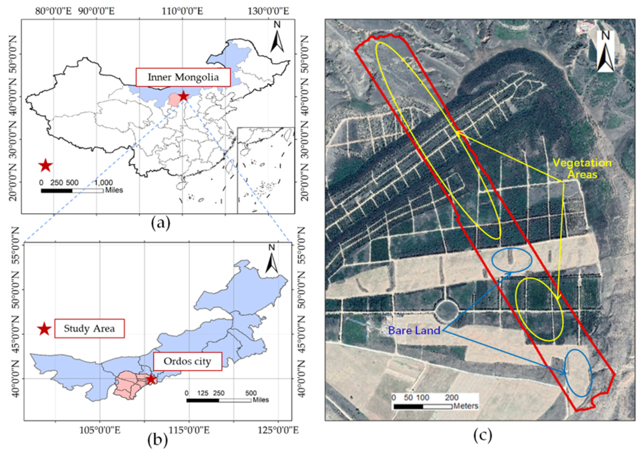
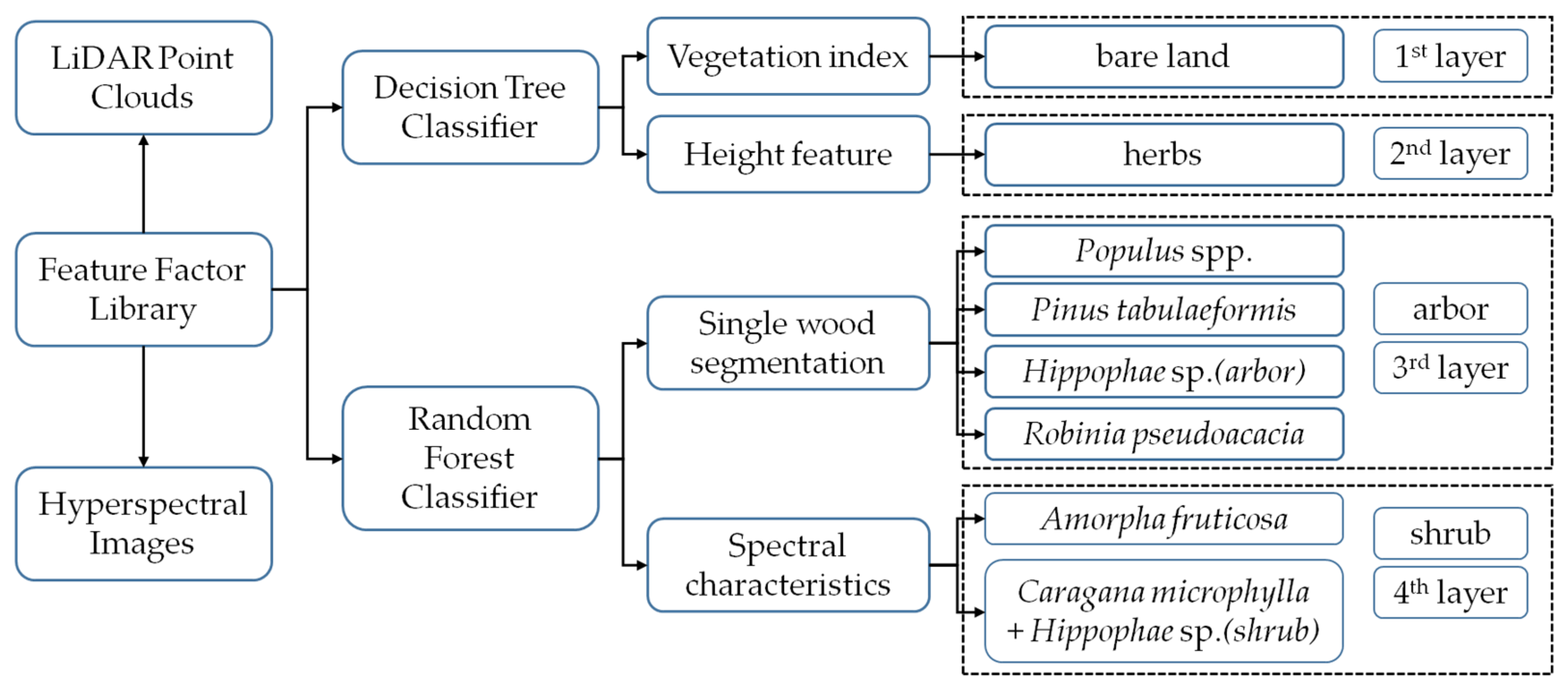
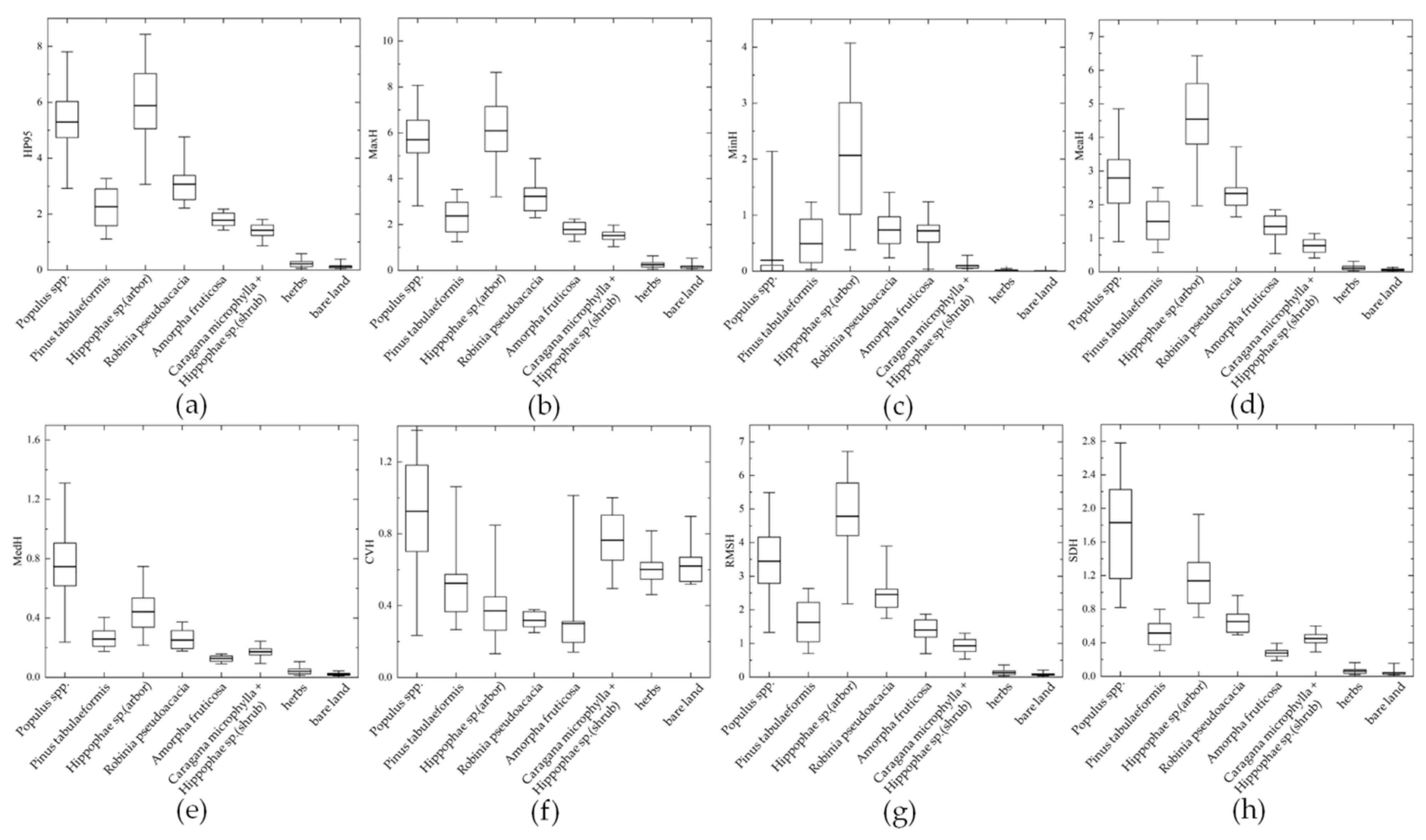

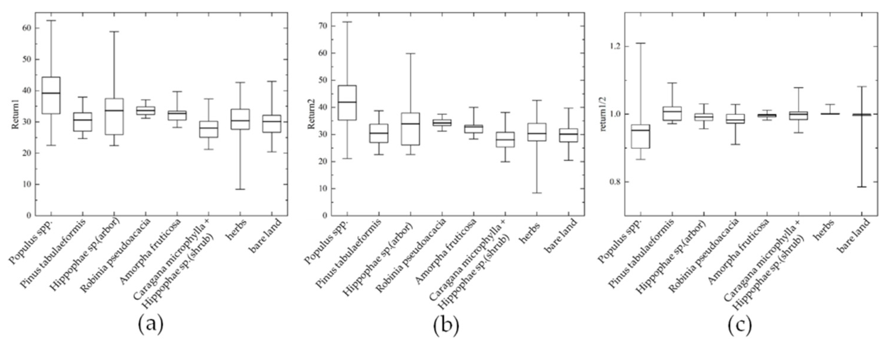
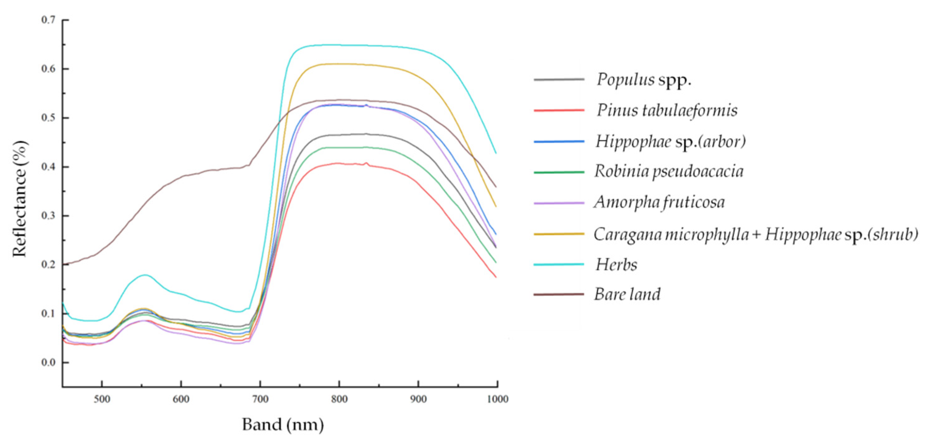
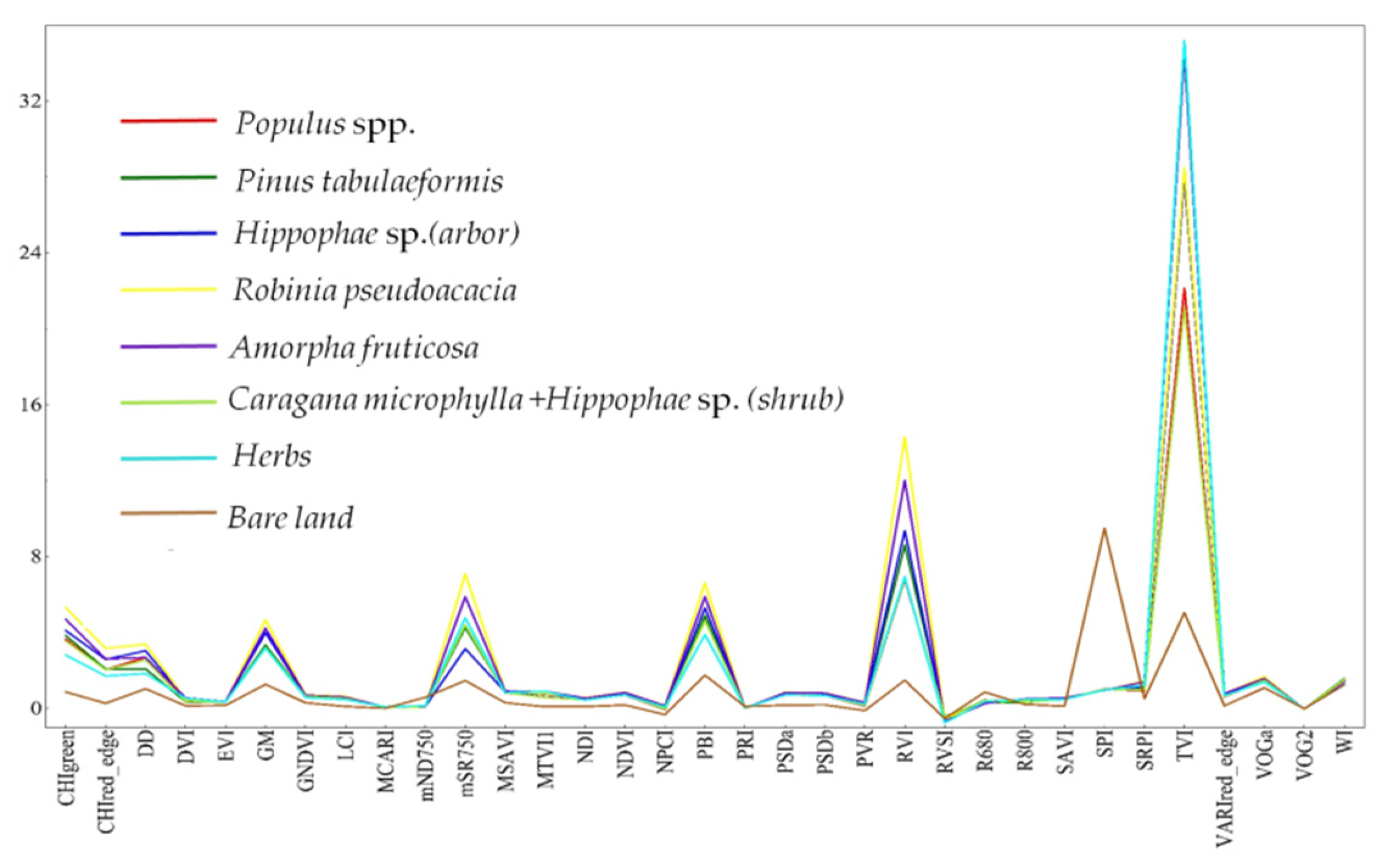
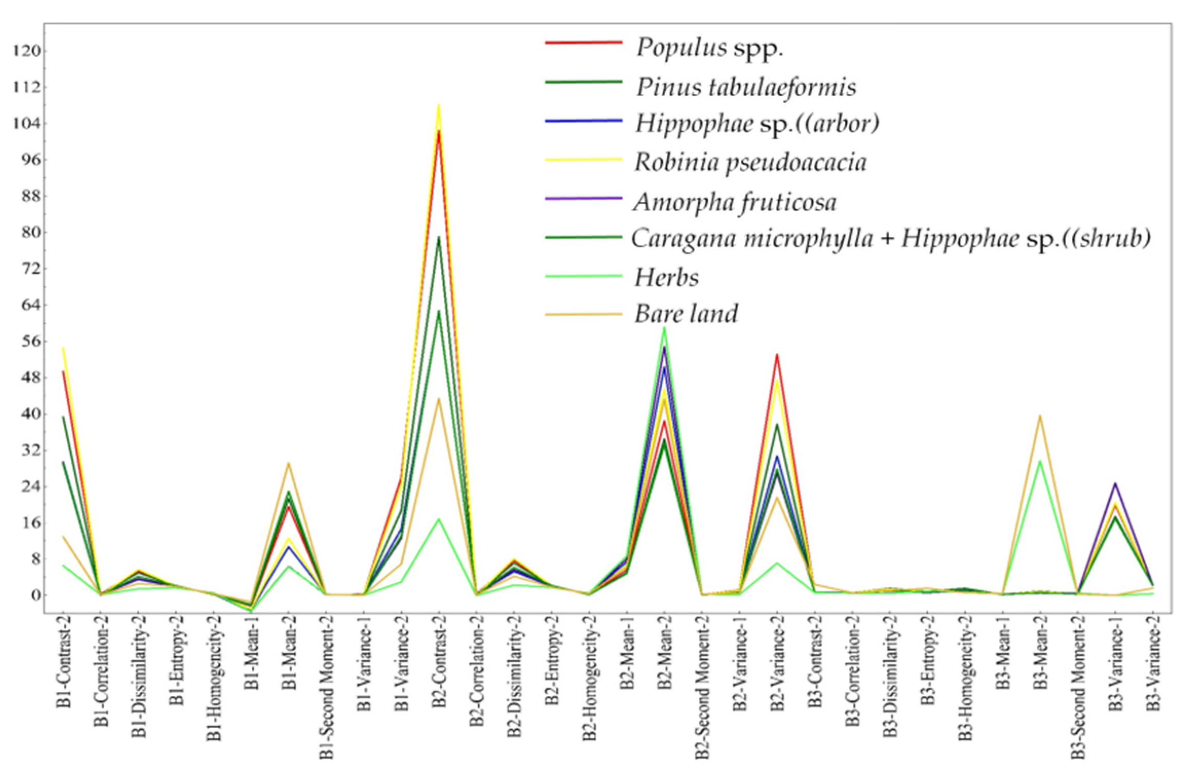
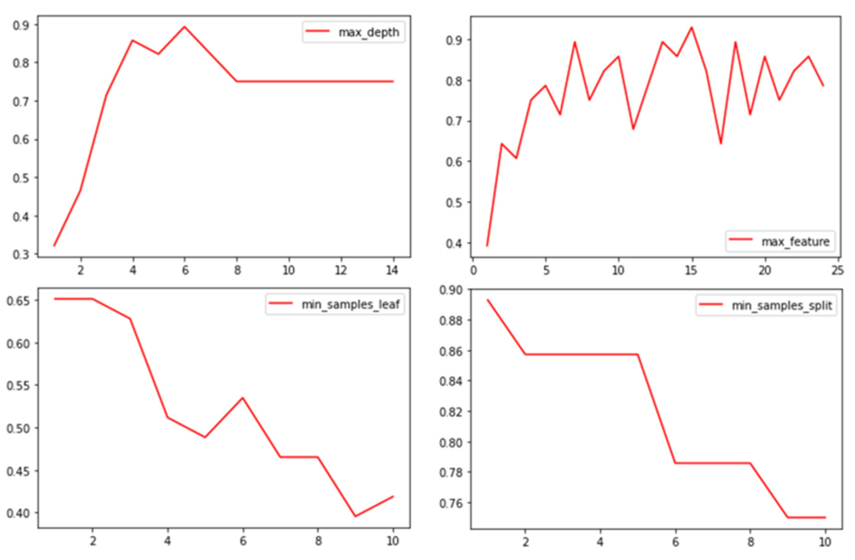
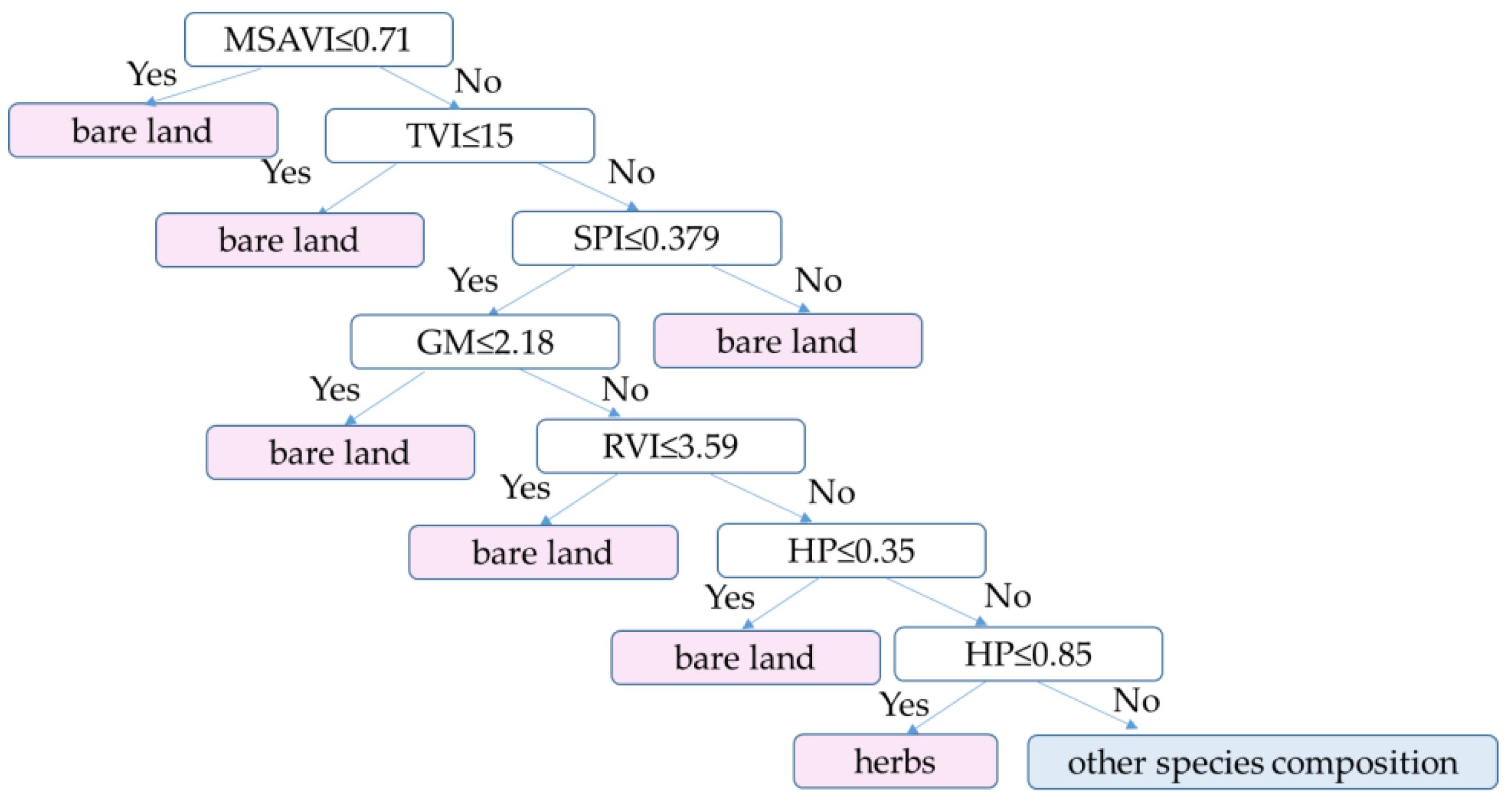

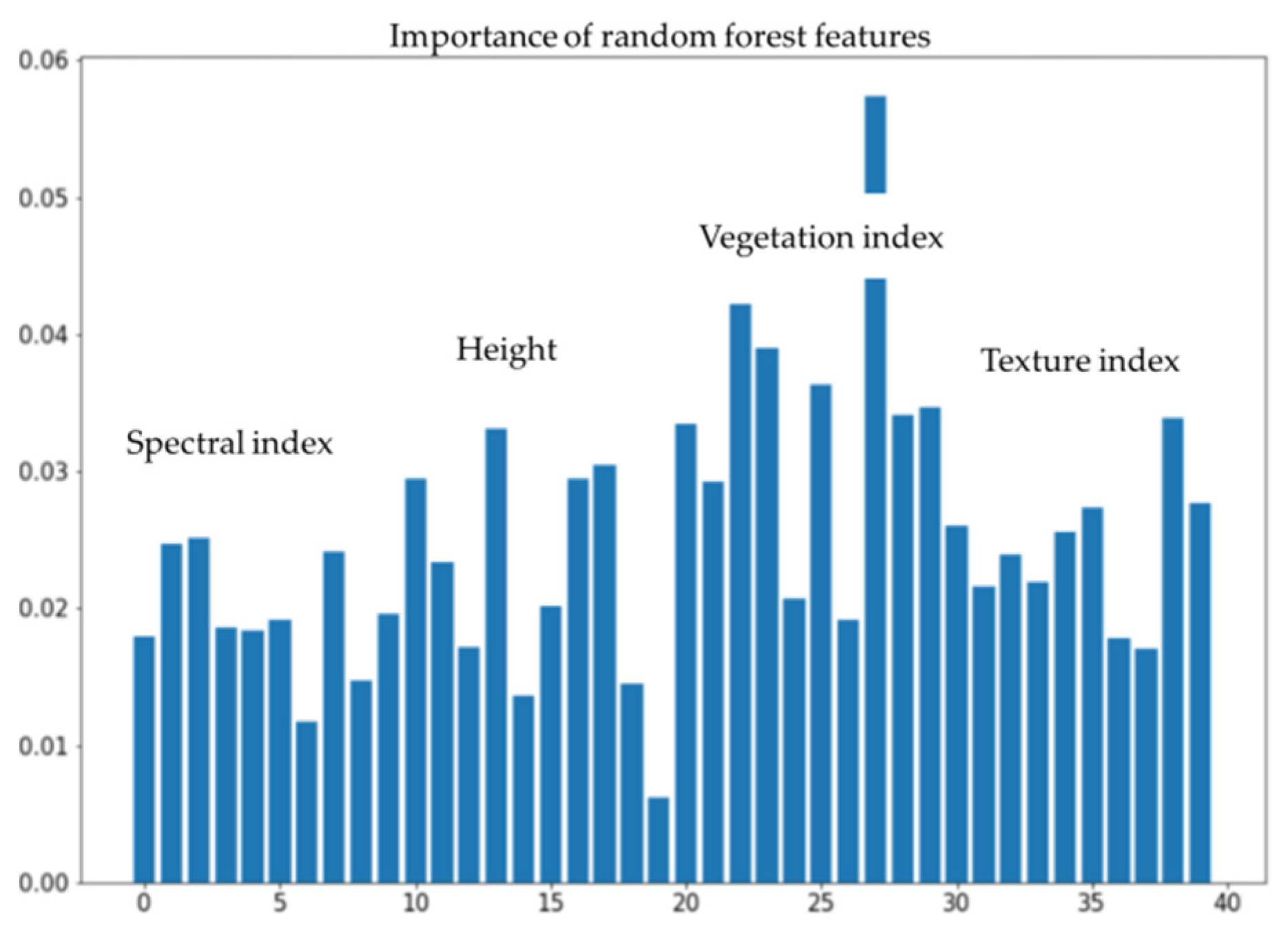
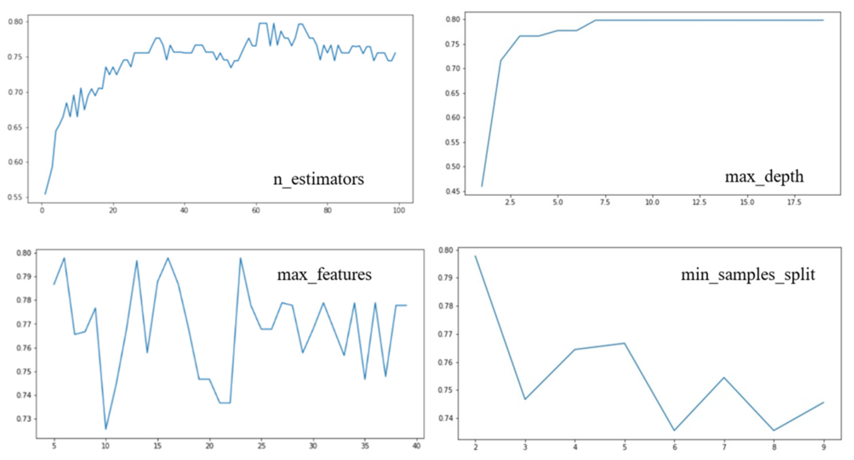
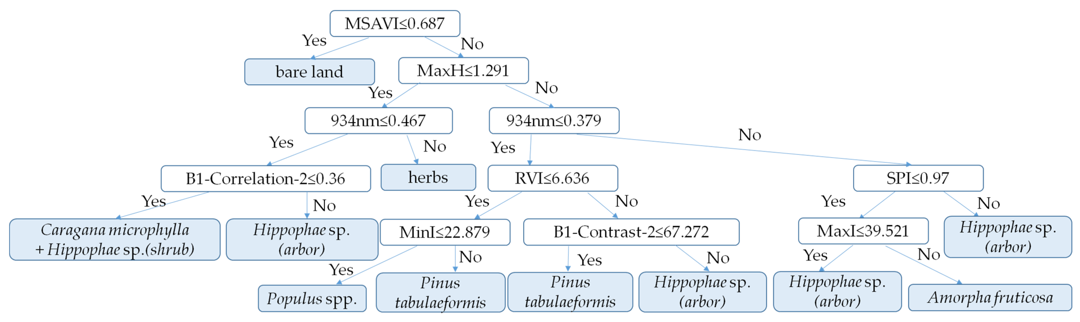
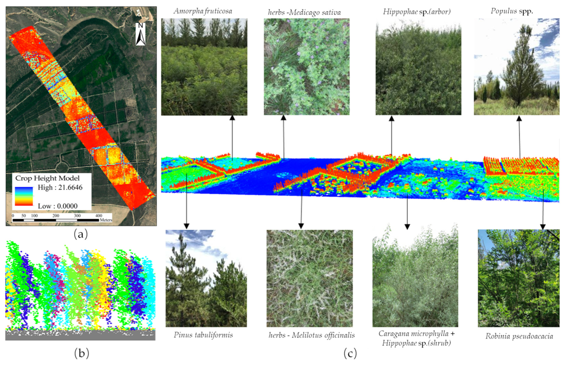
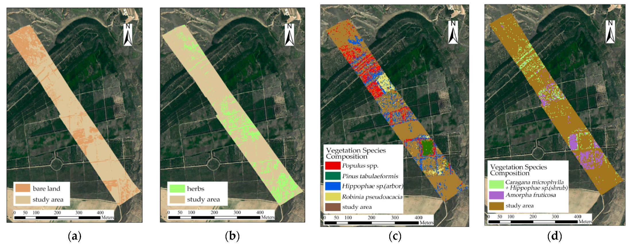
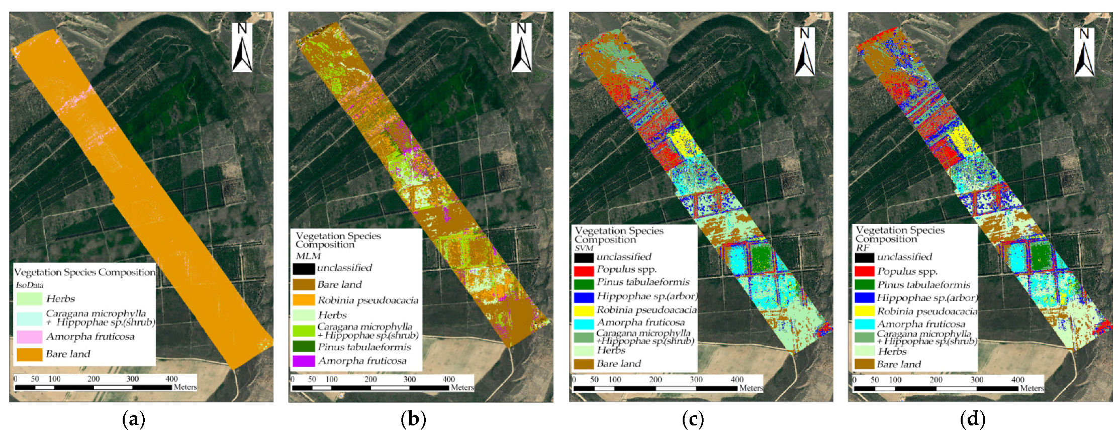
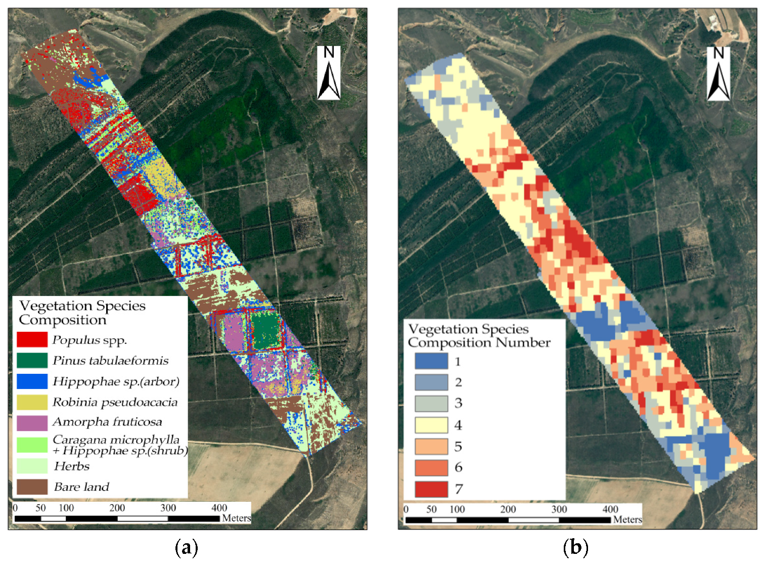
Publisher’s Note: MDPI stays neutral with regard to jurisdictional claims in published maps and institutional affiliations. |
© 2022 by the authors. Licensee MDPI, Basel, Switzerland. This article is an open access article distributed under the terms and conditions of the Creative Commons Attribution (CC BY) license (https://creativecommons.org/licenses/by/4.0/).