A Global Conversion Factor Model for Mapping Zenith Total Delay onto Precipitable Water

Abstract

The conversion factor is a key parameter for converting zenith wet delays (ZWD) into precipitable water vapour (PWV) with a mean value of 0.15, and the traditional method of calculating it is to model the weighted average temperature in the process of conversion factor calculation. Here, we overcome the dependence on high-precision atmospheric weighted average temperature for mapping ZWD onto PWV and build a global non-meteorological parametric model for conversion factor GΠ model by using the gridded data of global conversion factor time series from 2006 to 2013 provided by the Global Geodetic Observing System (GGOS) Atmosphere. Internal and external accuracy tests were performed using data from four times (UTC 00:00, 06:00, 12:00, and 18:00) per day throughout 2012 and 2014 as provided by the GGOS Atmosphere, and the statistical average root-mean-square (RMS) and mean absolute errors (MAE) on a global scale are 0.0031/0.0026 and 0.0030/0.0026, respectively, which only account for 1.5–2% of the conversion factor value. In addition, the observed GPS data are also used to validate the established GΠ model, and the RMS of the PWV differences between the established model and the observed meteorological data was less than 3.2 mm. The results show that the established GΠ model has a high accuracy, which can be used to calculate the PWV value where no observed meteorological parameters are available.

1. Introduction

It is important to understand the spatiotemporal variability of water vapour so as to study global climate change and for rainfall forecasting [1]. The traditional method of monitoring atmospheric water vapour mainly uses sounding balloons, water vapour radiometers, etc., but the data from the traditional method (such as the sounding balloons) have low temporal resolution, e.g., two or four times daily, and larger spatial resolution, e.g., 200 to 300 km [2,3]. In addition, water vapour radiometers are mainly affected by the weather and cannot work under rainfall or foggy weather conditions, and the instruments are unwieldy and expensive [4,5,6]. Therefore, traditional monitoring methods cannot meet the requirements of small- and medium-scale water vapour and weather monitoring tasks.

With the development of the global navigation satellite system (GNSS) technology, the monitoring of atmospheric water vapour by ground-based GNSS technology has become a new research hotspot. Satellite signals are delayed through the troposphere, including atmospheric dry delay and atmospheric wet delay. Askne and Nordius [4] first presented the approximate relationship between atmospheric moisture delay and precipitable water vapour (PWV) [1] and proposed a method of calculating atmospheric water vapour using ground-based GPS observations. Bevis et al. [7,8] first proposed the concept of GPS meteorology and presented basic methods for water vapour calculation based on satellite observations. The signal delay of the satellite to the ground station can be used to calculate atmospheric water vapour [9,10,11,12]. Compared to traditional methods, the GNSS technique has many advantages for atmospheric precipitation water vapour calculation: high spatial and temporal resolution, low cost, global coverage, all-weather operability, real-time data analysis, etc. Therefore, GNSS meteorological research has great practical value and development potential [13,14,15].

To obtain the PWV value, the zenith total delay (ZTD) and the zenith hydrostatic delay (ZHD) should be calculated, and then the zenith wet delay (ZWD), which is typically estimated as an unknown parameter in GNSS processing, can be extracted from the ZTD by subtracting the ZHD. Therefore, the PWV can be calculated by multiplying the conversion factor by the ZWD [16,17]. The conversion factor is mainly affected by the weighted average temperature, which is why many studies have been conducted on the weighted average temperature in the past. Ross and Rosenfeld [18] used radiosonde data from 13 stations over two years to simulate the equation of linear regression between the weighted average temperature $T_m$ and the land surface temperature $T_s$ in America [18]. The linear relationship offers good precision in mid-latitude areas; however, the equation established above has its limitations because not all GNSS stations are equipped with meteorological sensors [19,20]. Ross et al. [20] found that $T_m$ and $T_s$ are influenced by many factors such as location and season by analysing the 23-year data from 53 radiosonde stations around the world. Yao et al. [21] used global data from 135 radiosonde stations from 2005 to 2009 to establish the first-generation global weighted average temperature model ${\mathrm{GT}}_{\mathrm{m}}\text{-}\mathsf{{\rm I}}$. In 2013, the second-generation global weighted average temperature model ${\mathrm{GT}}_{\mathrm{m}}\text{-}\mathsf{{\rm I}}\mathsf{{\rm I}}$ was established which overcomes the data loss problem over sea areas when using the GPT model and the $T_m$ ~ $T_s$ relationship proposed by Bevis [3,21].

Here, we overcome the dependence on the high-precision atmospheric weighted average temperature in the process of the ZWD conversion to the PWV and establish a global non-meteorological parametric model for the conversion factor. The values of $T_m$ used to build the model were provided by the GGOS for the period from 2008 to 2013, with a time resolution of 6 hours (UTC 00:00, 06:00, 12:00, and 18:00) and a spatial resolution of 2.5° × 2°.

2. Method of Establishing the GΠ Model

The specific expression for calculating the PWV is as follows:

$$\begin{array}{l}\mathrm{PWV}=\mathsf{\Pi }\cdot \mathrm{ZWD}\\ \mathsf{\Pi }={10}^6\cdot {\left[(k_2^{\prime }+k_3/T_m)\cdot R_v\cdot {\rho }_w\right]}^{-1}\end{array}$$

(1)

where $\mathsf{\Pi }$ is the conversion factor, $k_2^{\prime }$ and $k_3$ represent the atmospheric refraction constant with values of 22.1 k/mb and 373,900 ${\mathrm{k}}^2/\mathrm{m}\mathrm{b}$, respectively [7], $R_V$ is a constant with a value of 461.495 $\mathrm{J}\cdot \mathrm{k}{\mathrm{g}}^{-1}\cdot {\mathrm{K}}^{-1}$, and ${\rho }_w$ is the water vapour density (g/cm³). $T_m$ represents the weighted average atmospheric temperature (unit: K). A linear relationship between the weighted average temperature and ground temperature was proposed by Bevis et al. [7,22,23] using radiosonde data over many years:

$$T_m=70.2+0.72T_s$$

(2)

where $T_s$ represents the ground temperature (unit: K) and the conversion error from the ZWD to the PWV is approximately 2% based on the above formula [7]. $\mathsf{\Pi }$ varies with season and latitude and has an approximate value of 0.15. According to Equation (1), the accuracy of atmospheric precipitation data is determined by the accuracy of the ZWD and $\mathsf{\Pi }$ [24]. The international GNSS service (IGS) can provide the ZTD with an RMS error of 1.5~5 mm while the ZHD can be estimated with an RMS error of a few millimetres by means of an empirical model using the surface-measured pressure. Therefore, a high-precision ZWD value can be obtained from GNSS observations with an RMS error of a few millimetres [25,26]. Once the ZWD is obtained, $\mathsf{\Pi }$ is the only key parameter to calculate the PWV; therefore, determining $\mathsf{\Pi }$ is a key issue in GNSS water vapour remote sensing [27].

2.1. Methods of Obtaining the Conversion Factor

As mentioned above, $\mathsf{\Pi }$ is related to $T_m$, while $T_m$ is related to the longitude and latitude, height of the station, and DoY (day of year); in addition, the given gas constant and atmospheric refraction constants are changed for different regions and times. Generally, there are several methods of obtaining the conversion factor. For the first method, $\mathsf{\Pi }$ can be regarded as a constant, usually taking a value of approximately 0.15 with a maximum range of 15%, which means 1 mm of the PWV corresponds to approximately 6.7 mm of the ZWD [28]. The above method is the simplest way to obtain $\mathsf{\Pi }$, but the accuracy of the estimated PWV is low. Therefore, the formula $T_m=70.2+0.72T_s$ or the local linear regression formula is usually used to calculate $T_m$, and then further used to calculate the conversion factor, which is considered as the second method.

In addition, $\mathsf{\Pi }$ can also be considered as a function of latitude, DoY, and expressed as follows [29]:

$${\mathsf{\Pi }}^{-1}=a_0+a_1\mathsf{\theta }+a_2\sin (2\mathsf{\pi }\frac{t_D}{365})+a_3\cos (2\mathsf{\pi }\frac{t_D}{365})$$

(3)

where $\mathsf{\theta }$ represents the latitude of the station, $t_D$ represents the DoY, $a_0=5.861$, $a_1=0.011$, $a_2=0.054$, and $a_3=0.138$; however, the above methods are not very accurate to express the conversion factor changes in different areas. Here, a global non-meteorological parametric model of the conversion factor is proposed based on the analysis of the factors influencing the conversion factor.

2.2. Analysis of the Conversion Factor

The time series of the global conversion factor data was analysed to determine the importance of those factors influencing the conversion factor. In our following analysis, the conversion factor was obtained from the GGOS Atmosphere with the temporal resolution of four times daily at UTC 00:00, 06:00, 12:00, and 18:00, respectively.

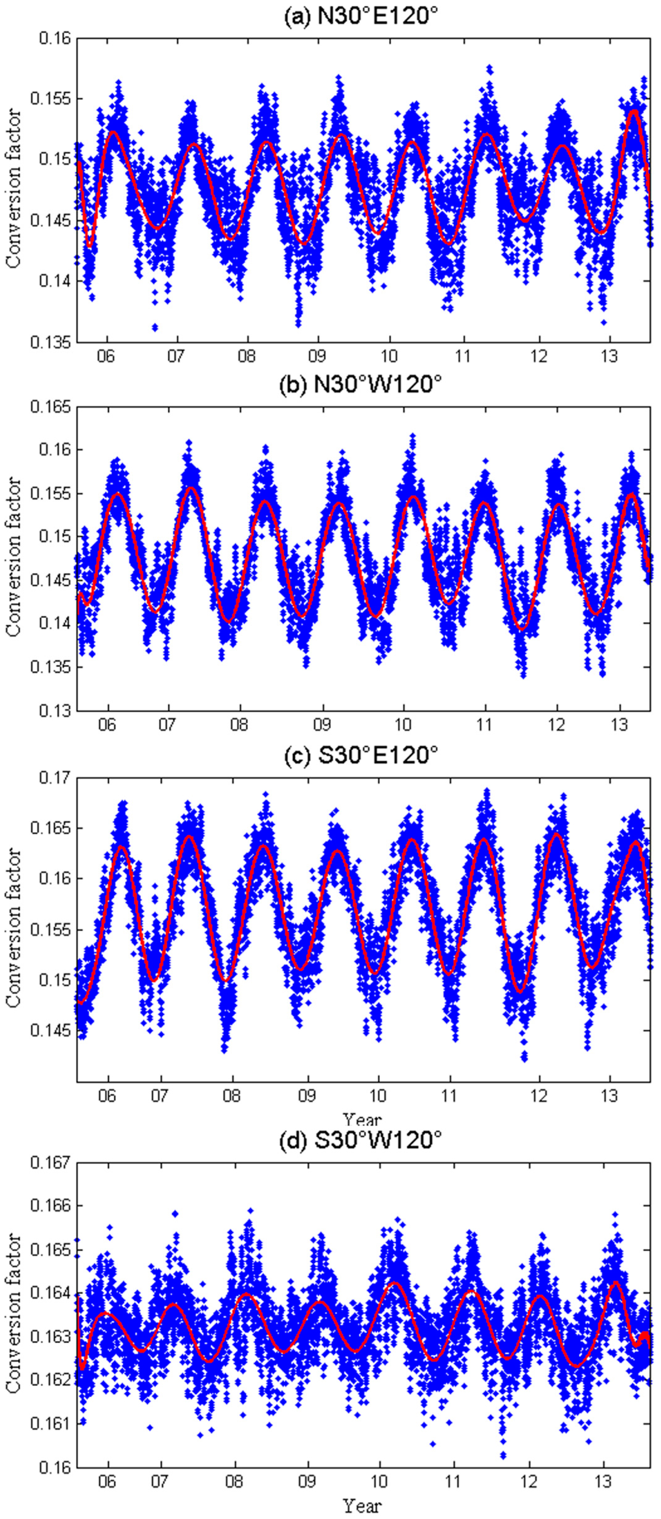
• Relationship between the conversion factor and the annual change.

The conversion factors at four specific locations (N30° E120°, N30° W120°, S30° E120°, and S30° W120°) were calculated using the 8-year data provided by the GGOS from 2006 to 2013, and Figure 1a–d shows the relationship between the conversion factor and the time in the four locations, respectively. It can be observed from Figure 1 that the conversion factor exhibits periodic changes with time, which suggests that the annual cycle is an important factor affecting the conversion factor; therefore, it should be considered when establishing the conversion factor model. The detected dependences of the conversion factor are expected since they reflect the dependences of the temperature.

2.

Relationship between the conversion factor and the semiannual change.

It is shown in Figure 1 that the conversion factor has a strong periodic relationship with the annual cycle. Therefore, the following experiments were carried out to determine whether or not the conversion factor is relative to the semiannual variation. The relationship between the conversion factor and the semiannual change was analysed using data from the year 2013. Figure 2a–d shows the changes of the conversion factor in four positions (N30° E120°, N30° W120°, S30° E120°, and S30° W120°), and the X axis refers to the DoY of 1 to 365, 2013. As can be seen from Figure 2, the conversion factor exhibits semiannual changes, which indicates that the semiannual change is another influential factor. Like the annual cycle, the semiannual cycle should also be considered when establishing the conversion factor model.

3.

Relationship between the conversion factor and the elevation.

To explore whether or not the conversion factor is related to elevation, the calculated conversion factor for the year 2013, on a global scale, was analysed for the effect of change in elevation. Figure 3 shows the conversion factor changes with altitude, and the trend is approximately linear at 0–4 km, while the trend disappears above 4 km. Due to the fact that most regions in the world lie at an elevation of less than 4 km, it is necessary to consider the elevation factor when establishing the conversion factor model [30]. In addition, some points well outside the linear relationship may be related to temperature, which remains to be further verified. It should be noted that not very many regions on Earth exist at these altitudes, and they correspond to dry regions of very low ZWD values with also low variability.

4.

Analysis of the modelling grid division.

Data with a spatial resolution of 2.5° × 2° provided by the GGOS Atmosphere were used to model the conversion factor; however, whether the conversion factor has a relationship with the latitude and longitude has yet to be determined. Therefore, it is necessary to analyse the correlation between the conversion factor and the latitude/longitude so as to ensure correctness of the model with regard to the adopted grid division method. Figure 4 and Figure 5 show the relationship between the conversion factor and the longitude/latitude, respectively, based on the conversion factor obtained from different longitudes and latitudes in 2013. It can be seen from Figure 4 and Figure 5 that the conversion factor has a strong relationship with the latitude and longitude; therefore, it is reasonable to establish the conversion factor using the grid division method. In addition, some outliers are observed, mainly due to the majority of elevations above 4000–5000 m (mainly the Himalayan region) being located in the latitude band.

2.3. Expression of the Conversion Factor Model

As described above, the conversion factor is affected by annual and semiannual effects and varies with height; thus, based on the above analysis, the following model was proposed:

$$\mathsf{\Pi }{=a}_1+a_{2}h+a_3\cos \left(2\mathsf{\pi }\frac{{doy\text{-}C}_1}{365.25}\right)+a_4\cos \left(4\mathsf{\pi }\frac{{doy\text{-}C}_2}{365.25}\right)+a_5\cos \left(2\mathsf{\pi }\frac{{hod\text{-}C}_3}{24}\right)$$

(4)

where $a_1$ represents the average value of the conversion factor, $a_2$ refers to the height vertical gradient, $h$ is the station height, $doy$ is day of year, $hod$ is hour of day (UTC time), $a_3,a_4,a_5$ represent annual, semiannual, and day period amplitudes, respectively, while $C_1,C_2,C_3$ represent annual, semiannual, and day period initial phases, respectively. The model coefficients can be estimated by using the least squares method.

The model coefficients were estimated in this paper using the grid data provided by the GGOS Atmosphere for 2008–2013. Figure 6a–d show the coefficients a2, a3, a4, and a5, respectively, while coefficient a1 is a constant with the value of about 0.0037. As can be seen from Figure 6a, the absolute value of a2 for the global conversion factor model is smaller on land and larger in marine areas while the absolute value of a3 is smaller at lower latitudes and larger at high latitudes except for some abnormal values near the equator (see Figure 6b); it can be seen in Figure 6c that the absolute value of the semiannual amplitude is larger in polar regions and smaller in the vicinity of the equator. In addition, the semiannual absolute amplitude appears to be larger in the northern hemisphere than that in the southern hemisphere, and the largest values occur over Siberia. As can be seen from Figure 6d, the absolute value of the diurnal amplitude is relatively large on land when compared to that over sea areas. In addition, opposite values appear in the eastern hemisphere (positive values) and western hemisphere (negative values): the reason for this may be that the diurnal amplitude is closely related to the daily temperature, so the opposite trend appears in the eastern and western hemispheres.

3. Result

Here, the root-mean-square (RMS) and mean absolute errors (MAE) are used as the standard for evaluating the established model as follows:

$$MAE=\frac{1}{N}{\displaystyle \sum _{\mathrm{i}=1}^N\left({\mathrm{x}}_{\mathrm{i}}-{\mathrm{x}}_{\mathrm{i}}^0\right)}$$

(5)

$$RMS=\sqrt{\frac{1}{N}{\displaystyle \sum _{\mathrm{i}=1}^N{\left({\mathrm{x}}_{\mathrm{i}}-{\mathrm{x}}_{\mathrm{i}}^0\right)}^2}}$$

(6)

where ${\mathrm{x}}_{\mathrm{i}}$ represents the estimated value of the G$\mathsf{\Pi }$ model while ${\mathrm{x}}_{\mathrm{i}}^0$ refers to the true value calculated using the GGOS data and $N$ represents the total number of observed values; MAE can be used to embody the degree of deviation of the estimated value from the true value, while RMS is used to measure the reliability of the established model. In the following Section 3.1 and Section 3.2, the internal accuracy testing is performed for the period of the data used in the determination of the conversion factor model while the external accuracy is carried out using the GGOS data over a period not used in this analysis.

3.1. Internal Accuracy Testing

To validate the internal accuracy of the established model, the conversion factor derived from the G$\mathsf{\Pi }$ model four times daily (UTC 00:00, 06:00, 12:00, and 18:00) in 2012 was compared to those values globally derived from the GGOS data with a spatial resolution of 2.5° × 2°. Figure 7 shows the internal accuracy of the (a) MAE and (b) RMS of the G$\mathsf{\Pi }$ model while

Table 1. Statistics results: internal accuracy testing of the GΠ model.

Model	MAE			RMS
	Mean	Max	Min	Mean	Max	Min
GΠ	0.0026	0.026	0.0005	0.0031	0.0317	0.0006

lists the statistical results on a global scale.

It can be seen from Table 1 that the estimated value of the conversion factor calculated using the G$\mathsf{\Pi }$ model was closer to that derived from the GGOS data, and the magnitude of internal accuracy was 10⁻³. It also can be seen from Figure 7 that the RMS and MAE range from 0 to 0.0317 and from 0 to 0.026 on the global scale, which indicates a good accuracy in the G$\mathsf{\Pi }$ model; however, some abnormal values appeared near the equator, which may have been affected by the El Niño event at that time [31].

3.2. External Accuracy Testing

To assess the external accuracy of the G$\mathsf{\Pi }$ model, the conversion factor derived from the established G$\mathsf{\Pi }$ model in 2004 was compared with that from the GGOS data at four times each day (UTC 00:00, 06:00, 12:00, and 18:00) on a global scale. Statistical results are shown in

Table 2. Statistical results: external accuracy testing of the GΠ model.

Model	MAE			RMS
	Mean	Max	Min	Mean	Max	Min
GΠ	0.0026	0.0244	0.0005	0.0030	0.0304	0.0006

, while Figure 8 shows the distribution of the MAE and RMS. It also can be concluded from

Table 3. Statistical results: MAE and RMS for the GΠ model across different height ranges in 2014.

Height Range (m)	MAE			RMS
	Mean (10−3)	Max (10−3)	Min (10−3)	Mean (10−3)	Max (10−3)	Min (10−3)
<500	2.5	24.4	0.5	2.9	30.4	0.6
500~1000	2.9	19.5	0.6	3.4	22.1	0.7
1000~2000	3	7.7	0.5	3.5	8.9	0.7
>2000	3	7.9	0.7	3.6	9.1	0.9

and Figure 8 that the validated result is similar to that arising from internal testing.

The compared result was further analysed to obtain the distribution of the RMS. Figure 9 shows the histogram of the average RMS of external accuracy testing for the G$\mathsf{\Pi }$ model. It can be observed that most RMS values were less than 0.005, which suggests that the G$\mathsf{\Pi }$ model provides a good model to the GGOS data.

To analyse the accuracy of the G$\mathsf{\Pi }$ model at different heights, longitudes, and latitudes, the external accuracy of the MAE and RMS was calculated, and the statistical results are shown in Table 3,

Table 4. Statistical results: MAE and RMS for the GΠ model across different latitude ranges in 2014.

Longitude Range	MAE			RMS
	Mean (10−3)	Max (10−3)	Min (10−3)	Mean (10−3)	Max (10−3)	Min (10−3)
0°~30°	2	24.4	0.5	2.3	30.4	0.6
30°~60°	2.4	10.2	0.6	2.9	11.6	0.8
60°~90°	2.7	22.5	0.5	3.2	30.4	0.6
90°~120°	2.8	11.5	0.5	3.4	13	0.6
120°~150°	2.7	21.8	0.5	3.2	24.8	0.6
150°~180°	2.4	6.3	0.6	2.8	7.5	0.8

and

Table 5. Statistical results: MAE and RMS for the GΠ model across different longitude ranges in 2014.

Latitude Range	MAE			RMS
	Mean (10−3)	Max (10−3)	Min (10−3)	Mean (10−3)	Max (10−3)	Min (10−3)
0°~30°	1.4	24.4	0.5	1.7	30.4	0.6
30°~60°	2.8	7.8	1.1	3.3	9.1	1.4
60°~90°	3.7	8.1	1.3	4.3	9.4	1.6

and Figure 9.

It can be observed from Table 3 that the average MAE and RMS of the G$\mathsf{\Pi }$ model increased with height, which suggests that the conversion factor is influenced by altitude. Table 4 shows that the average MAE and RMS of the G$\mathsf{\Pi }$ model presented an increasing trend with longitude and then decreased, while the values of the MAE and RMS were largest in the 90°~120° longitude. Table 5 shows that the average values of the MAE and RMS increased with latitude. In Figure 10a–f, a few larger MAE and RMS values are found at heights of up to 1000 m, within 60°W to 60°E longitudes and at 30°N to 30°S latitudes: this phenomenon may be caused by the El Niño event. In addition, the overall accuracy of the G$\mathsf{\Pi }$ model is high at low latitudes and low longitudes and relatively poor over high latitude and high longitude ranges.

3.3. Case Study

To verify the accuracy of the established G$\mathsf{\Pi }$ model, comparisons for stations HKSC and ANJI in the CORS network of Hong Kong and Zhejiang Province were conducted. THKSC and ANJI were selected because the large PWV values existed for the whole year at those stations, which can reflect the real performance of proposed model. In addition, the collocated meteorological stations existed at those two stations, and the high-precision PWV could be obtained as the reference. The data for the whole year of 2014 from HKSC and for the period from 1 May to 20 July 2015 from the ANJI site were selected. The specific location and height of the two selected stations are given in

Table 6. Location and height of the selected stations.

Station	HKSC			ANJI
	Lat. (°)	Lon. (°)	Height (m)	Lat. (°)	Lon. (°)	Height (m)
Value	22.32	114.13	20.15	30.37	119.41	35.40

. The high-precision PWV data were calculated using GPS observations and the observed meteorological data based on the method proposed in Section 2 (met-derived PWV). In our experiment, the precise pointing positioning (PPP) technique [32,33] was used to process the GPS observations using the conventional ionosphere-free (IF) code and phase measurements. The receiver coordinates, the tropospheric zenith wet delay, the receiver clock error, and the IF phase ambiguities were regarded as unknown parameters, which were estimated using the extended Kalman filter. The global pressure and temperature (GPT) model [34] was used to obtain the meteorological parameter (pressure) while the Saastamoinen model was introduced to calculate the tropospheric hydrostatic delay [35]. The corresponding meteorological data were checked before use. In addition, the PWV values were also calculated using the values of parameter $\mathsf{\Pi }$ estimated on the basis of the established model (model-derived PWV). It is worth mentioning that the final estimated parameter $\mathsf{\Pi }$ was based on the re-established model, which excludes the outliers mentioned in Section 3.2.

Two kinds of PWV values were compared as shown in Figure 11, where (a) and (b) provide comparisons of the PWV time series. It can be observed that the model-derived PWV time series was consistent with the met-derived PWV time series. In addition, it can be concluded that the PWV difference increased with increasing PWV values. If the met-derived PWV is considered as a reference, the RMS of the model-derived PWV for the ANJI site is 2.95 mm while the STD and bias are 1 mm and 2.77 mm, respectively. For the HKSC station, the RMS of the model-derived PWV was 3.18 mm while the STD and bias were 1.6 mm and 2.75 mm, respectively. It can also be seen from Figure 10a,b that the PWV differences for the two sites were small when the PWV values were relatively low (i.e., below 40 mm) while the differences increased with increasing PWV. The analysis shows that there was a small systemic bias between the met-derived PWV and the model-derived PWV, which may be due to the failure to consider all factors when building the G$\mathsf{\Pi }$ model. Generally, the G$\mathsf{\Pi }$ model established in this research has a high precision and can be used for the calculation of the PWV in the absence of meteorological parameters.

4. Discussion

It can be observed from the internal and external validations that the proposed model has a good performance on the global scale. However, some outliers appeared around the equator both in internal and external experiments, and such result may be related to the GGOS data used for modeling and affected by the El Niño event at that time [31]. It can also be found that coefficient a3 of the established global conversion factors globally estimated using the least squares method (Figure 6) also shows the similar distribution as that of the MAE and RMS in internal and external validations; it means that the outliers are mainly affected by coefficient a3 of the established global conversion factors in Equation (4). Coefficient a3 is the annual phases of the global conversion factors highly related to the global climate change; therefore, the occurrence of the El Niño event may have an evident influence on coefficient a3.

Two stations in Zhejiang province and Hong Kong were used to further validate the proposed global conversion factor model, and the experimental result also shows the good performance of the proposed model. Although those two stations cannot fully evaluate the performance of the proposed global conversion factor model, the selected two stations have relatively high PWV values with the average PWV of approximately 40 mm. Due to this paper being mainly focused on the establishment of the global conversion factor model, more attentions was paid to the modeling. In addition, internal and external accuracy validations of the proposed model on a global scale using the GGOS data were performed, which proved the good performance of the proposed model. Therefore, only the case with two stations was used to perform the application experiment.

5. Conclusions

A global conversion factor model of non-meteorological parameters (G$\mathsf{\Pi }$ model) was established by using gridded data provided by the GGOS Atmosphere from 2006 to 2014. The established model considers the changes of the annual, semiannual, and day atmospheric water vapour; in addition, this model is also related to longitude, latitude, and height. The internal accuracy of the established model was tested using the data from 2012 provided by the GGOS Atmosphere, and the result shows that the average values of the MAE and RMS of the G$\mathsf{\Pi }$ model were 0.0026 and 0.0031 respectively. The external accuracy was also tested by using data provided by the GGOS in 2014, and the result shows that the average values of the MAE and RMS of the established G$\mathsf{\Pi }$ model were 0.0026 and 0.0030, respectively. Those validated results reveal that the established G$\mathsf{\Pi }$ model based on the GGOS Atmosphere data offers high precision, and the internal and external accuracies are of the order of magnitude of 10⁻³, which accounts for only 1.5–2% of the conversion factor value. To validate the applicability of the established G$\mathsf{\Pi }$ model, a case study was assessed that involved two sites in different regions with large PWV values for the whole year over different time periods. The statistical results from both sites revealed that the RMS error of the PWV calculated based on the established G$\mathsf{\Pi }$ model was about 3 mm; in addition, the model coefficient could be easily obtained at a specific grid point and the conversion factor was directly obtained, which was of significance for the calculation of the PWV, especially when faced with the unavailability of meteorological parametric data.

References

1. Yao, Y.; Shan, L.; Zhao, Q. Establishing a method of short-term rainfall forecasting based on GNSS-derived PWV and its application. Sci. Rep. 2017, 7, 12465. [Google Scholar] [CrossRef] [PubMed]
2. Wong, M.S.; Jin, X.; Liu, Z.; Nichol, J.; Chan, P.W. Multi-sensors study of precipitable water vapour over mainland China. Int. J. Climatol. 2015, 35, 3146–3159. [Google Scholar] [CrossRef]
3. Yao, Y.B.; Zhang, B.; Yue, S.Q.; Xu, C.Q.; Peng, W.F. Global empirical model for mapping zenith wet delays onto precipitable water. J. Geod. 2013, 87, 439–448. [Google Scholar] [CrossRef]
4. Askne, J.; Nordius, H. Estimation of tropospheric delay for microwaves from surface weather data. Radio Sci. 1987, 22, 379–386. [Google Scholar] [CrossRef]
5. Duan, J.; Bevis, M.; Fang, P.; Bock, Y.; Chiswell, S.; Businger, S.; Rocken, C.; Solheim, F.; van Hove, T.; Ware, R.; et al. GPS meteorology: Direct estimation of the absolute value of precipitable water. J. Appl. Meteorol. Climatol. 1996, 35, 830–838. [Google Scholar] [CrossRef] [Green Version]
6. Flores, A.; Ruffini, G.; Rius, A. 4D tropospheric tomography using GPS slant wet delays. Ann. Geophys. 2000, 18, 223–234. [Google Scholar] [CrossRef]
7. Bevis, M.; Businger, S.; Herring, T.A.; Rocken, C.; Anthes, R.A.; Ware, R.H. GPS meteorology: Remote sensing of atmospheric water vapor using the Global Positioning System. J. Geophys. Res. Atmos. 1992, 97, 15787–15801. [Google Scholar] [CrossRef]
8. Bevis, M.; Businger, S.; Chiswell, S.; Herring, T.A.; Anthes, R.A.; Rocken, C.; Ware, R.H. GPS meteorology: Mapping zenith wet delays onto precipitable water. J. Appl. Meteorol. 1994, 33, 379–386. [Google Scholar] [CrossRef]
9. Bi, Y.; Mao, J.; Li, C. Preliminary results of 4-D water vapor tomography in the troposphere using GPS. Adv. Atmos. Sci. 2006, 23, 551–560. [Google Scholar] [CrossRef]
10. Chen, J. On the error analysis for the remote sensing of atmospheric water vapor by ground based GPS. Acta Geod. Cartogr. Sin. 1998, 27, 113–118. [Google Scholar]
11. Rocken, C.; Hove, T.V.; Johnson, J.; Solheim, F.; Ware, R.; Bevis, M.; Chiswell, S.; Businger, S. GPS/STORM—GPS sensing of atmospheric water vapor for meteorology. J. Atmos. Ocean. Technol. 1995, 12, 468–478. [Google Scholar] [CrossRef]
12. Rocken, C.; Ware, R.; Van Hove, T.; Solheim, F.; Alber, C.; Johnson, J.; Bevis, M.; Businger, S. Sensing atmospheric water vapor with the Global Positioning System. Geophys. Res. Lett. 1993, 20, 2631–2634. [Google Scholar] [CrossRef] [Green Version]
13. Fernandes, M.J.; Lázaro, C.; Nunes, A.L.; Pires, N.; Bastos, L.; Mendes, V.B. GNSS-derived path delay: An approach to compute the wet tropospheric correction for coastal altimetry. IEEE Geosci. Remote Sens. Lett. 2010, 7, 596–600. [Google Scholar] [CrossRef]
14. Fernandes, M.J.; Lázaro, C.; Ablain, M.; Pires, N. Improved wet path delays for all ESA and reference altimetric missions. Remote Sens. Environ. 2015, 169, 50–74. [Google Scholar] [CrossRef] [Green Version]
15. Fernandes, M.J.; Lázaro, C. GPD+ wet tropospheric corrections for CryoSat-2 and GFO altimetry missions. Remote Sens. 2016, 8, 851. [Google Scholar] [CrossRef] [Green Version]
16. Vázquez, B.G.E.; Grejner-Brzezinska, D.A. GPS-PWV estimation and validation with radiosonde data and numerical weather prediction model in Antarctica. GPS Solut. 2013, 17, 29–39. [Google Scholar] [CrossRef]
17. Liu, J.; Sun, Z.; Liang, H.; Xu, X.; Wu, P. Precipitable water vapor on the Tibetan Plateau estimated by GPS, water vapor radiometer, radiosonde, and numerical weather prediction analysis and its impact on the radiation budget. J. Geophys. Res. Atmos. 2005, 110, 1–11. [Google Scholar] [CrossRef]
18. Tregoning, P.; Herring, T.A. Impact of a priori zenith hydrostatic delay errors on GPS estimates of station heights and zenith total delays. Geophys. Res. Lett. 2006, 33, 1–5. [Google Scholar] [CrossRef] [Green Version]
19. Mendes, V.B. Modeling the neutral-atmospheric propagation delay in radiometric space techniques. UNB Geod. Geomat. Eng. Tech. Rep. 1999, 199, 10. [Google Scholar]
20. Ross, R.J.; Rosenfeld, S. Estimating mean weighted temperature of the atmosphere for Global Positioning System applications. J. Geophys. Res. Atmos. 1997, 102, 21719–21730. [Google Scholar] [CrossRef] [Green Version]
21. Saastamoinen, J. Atmospheric correction for the troposphere and stratosphere in radio ranging satellites. Use Artif. Satell. Geod. 1972, 15, 247–251. [Google Scholar]
22. Byun, S.H.; Bar-Sever, Y.E. A new type of troposphere zenith path delay product of the international GNSS service. J. Geod. 2009, 83, 1–7. [Google Scholar] [CrossRef] [Green Version]
23. Mendes, V.B.; Prates, G.; Santos, L.; Langley, R.B. An evaluation of the accuracy of models for the determination of the weighted mean temperature of the atmosphere. In Proceedings of the 2000 National Technical Meeting of The Institute of Navigation, Anaheim, CA, USA, 26–28 January 2000; pp. 433–438. [Google Scholar]
24. Kouba, J. A Guide to Using International GNSS Service (IGS) Products. 2009. Available online: http://igscb.jpl.nasa.gov/igscb/resource/pubs/UsingIGSProductsVer21.pdf (accessed on 22 January 2022).
25. Fernandes, M.J.; Pires, N.; Lázaro, C.; Nunes, A.L. Tropospheric delays from GNSS for application in coastal altimetry. Adv. Space Res. 2013, 51, 1352–1368. [Google Scholar] [CrossRef]
26. Notarpietro, R.; Cucca, M.; Gabella, M.; Venuti, G.; Perona, G. Tomographic reconstruction of wet and total refractivity fields from GNSS receiver networks. Adv. Space Res. 2011, 47, 898–912. [Google Scholar] [CrossRef]
27. Yao, Y.B.; Zhu, S.; Yue, S.Q. A globally applicable, season-specific model for estimating the weighted mean temperature of the atmosphere. J. Geod. 2012, 86, 1125–1135. [Google Scholar] [CrossRef]
28. MacDonald, A.E.; Xie, Y.; Ware, R.H. Diagnosis of three-dimensional water vapor using a GPS network. Mon. Weather Rev. 2002, 130, 386–397. [Google Scholar] [CrossRef]
29. Zhang, S. Research and Application of Remote Sensing Water Vapor Using Ground Based GPS/Met. Ph.D. Thesis, Wuhan University, Wuhan, China, 2009. [Google Scholar]
30. Kouba, J. Implementation and testing of the gridded Vienna Mapping Function 1 (VMF1). J. Geod. 2008, 82, 193–205. [Google Scholar] [CrossRef]
31. Jin, S.; Park, J.U.; Cho, J.H.; Park, P.H. Seasonal variability of GPS-derived zenith tropospheric delay (1994–2006) and climate implications. J. Geophys. Res. Atmos. 2007, 112, 1–11. [Google Scholar] [CrossRef]
32. Zumberge, J.F.; Heflin, M.B.; Jefferson, D.C.; Watkins, M.M.; Webb, F.H. Precise point positioning for the efficient and robust analysis of GPS data from large networks. J. Geophys. Res. Solid Earth 1997, 102, 5005–5017. [Google Scholar] [CrossRef] [Green Version]
33. Kouba, J.; Héroux, P. Precise point positioning using IGS orbit and clock products. GPS Solut. 2001, 5, 12–28. [Google Scholar] [CrossRef]
34. Böhm, J.; Niell, A.; Tregoning, P.; Schuh, H. Global Mapping Function (GMF): A new empirical mapping function based on numerical weather model data. Geophys. Res. Lett. 2006, 33, 1–4. [Google Scholar] [CrossRef] [Green Version]
35. Saastamoinen, J. Contributions to the theory of atmospheric refraction. Bull. Géod. (1946–1975) 1972, 105, 279–298. [Google Scholar] [CrossRef]
Figure 1. Changes of the conversion factors with time over the period from 2006 to 2013 at the four selected locations of (a) N30° E120°, (b) N30° W120°, (c) S30° E120° and (d) S30° W120°, globally.
Remotesensing 14 01086 g001
Figure 2. Relationship between the conversion factor and the semiannual change at the four selected locations of (a) N30° E120°, (b) N30° W120°, (c) S30° E120° and (d) S30° W120° using the data from the year 2013.
Remotesensing 14 01086 g002
Figure 3. Relationship between the conversion factor and the elevation globally using the data from the year 2013.
Remotesensing 14 01086 g003
Figure 4. Relationship between the conversion factor and the longitude using the data of grid points globally from the year 2013.
Remotesensing 14 01086 g004
Figure 5. Relationship between the conversion factor and the latitude using the data of grid points globally from the year 2013.
Remotesensing 14 01086 g005
Figure 6. Coefficients distribution of the established global conversion factors globally estimated using the least squares method, where (ad) represent the distribution of coefficients a2, a3, a4, and a5, respectively.
Remotesensing 14 01086 g006
Figure 7. Distribution of the (a) MAE and (b) RMS: internal accuracy testing of the GΠ model when compared with that from the GGOS data of 2012.
Remotesensing 14 01086 g007
Figure 8. Distribution of the (a) MAE and (b) RMS: external accuracy testing of the GΠ model when compared with that from the GGOS data of 2014.
Remotesensing 14 01086 g008
Figure 9. Histogram of the average RMS of external accuracy testing for the GΠ model when compared with that from the GGOS data of 2014.
Remotesensing 14 01086 g009
Figure 10. Distribution of the MAE and RMS with respect to height, latitude, and longitude in 2004, where (a,b) refer to the MAE and RMS with height, (c,d) are the MAE and RMS with the latitude while the (e,f) represent the MAE and RMS with longitude, respectively.
Remotesensing 14 01086 g010
Figure 11. Comparison of the met-derived and model-derived PWV for the two selected stations, where (a) is the PWV comparison of ANJI station with the data from 1 May to 20 July 2015 while (b) is the PWV comparison of HKSC station with the data for the whole year of 2014.
Remotesensing 14 01086 g011