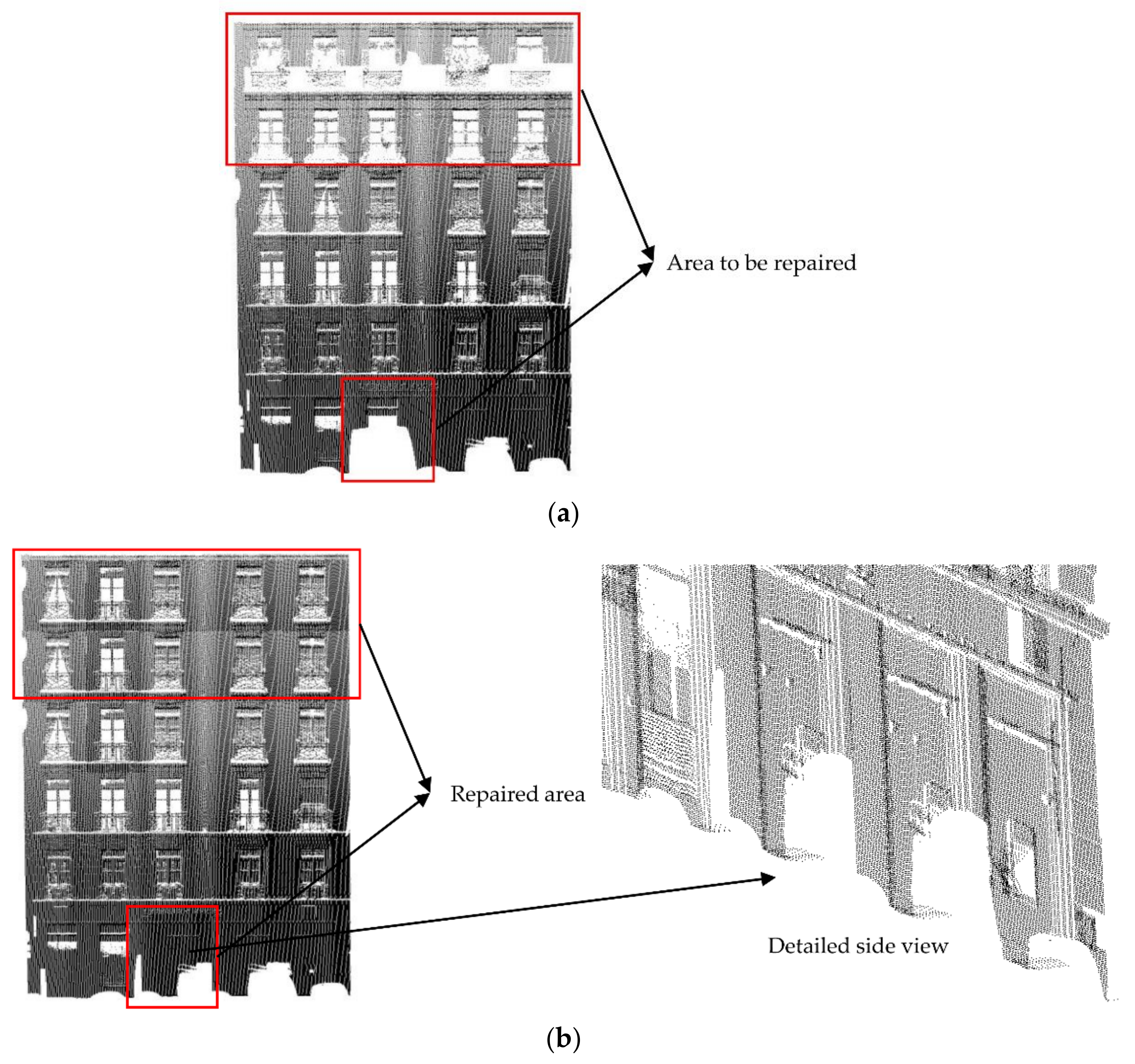
Abstract
The integrity of point cloud is the basis for smoothly ensuring subsequent data processing and application. For “Smart City” and “Scan to Building Information Modeling (BIM)”, complete point cloud data is essential. At present, the most commonly used methods for repairing point cloud holes are multi-source data fusion and interpolation. However, these methods either make it difficult to obtain data, or they are ineffective at repairs or labor-intensive. To solve these problems, we proposed a point cloud “fuzzy” repair algorithm based on the distribution regularity of buildings, aiming at the façade of a building in an urban scene, especially for the vehicle Lidar point cloud. First, the point cloud was rotated to be parallel to the plane XOZ, and the feature boundaries of buildings were extracted. These boundaries were further classified as horizontal or vertical. Then, the distance between boundaries was calculated according to the Euclidean distance, and the points were divided into grids based on this distance. Finally, the holes in the grid that needed to be repaired were filled from four adjacent grids by the “copy–paste” method, and the final hole repairs were realized by point cloud smoothing. The quantitative results showed that data integrity improved after the repair and conformed to the state of the building. The angle and position deviation of the repaired grid were less than 0.54° and 3.25 cm, respectively. Compared with human–computer interaction and other methods, our method required less human intervention, and it had high efficiency. This is of promotional significance for the repair and modeling of point cloud in urban buildings.
1. Introduction
With the rapid development of Lidar technology and the “Smart City”, using Lidar to obtain the point cloud of urban scenes or model urban buildings is becoming increasingly popular [1,2,3,4,5]. The “Scan to BIM” technology is also widely used in various applications related to the “Smart City”, such as city positioning [6,7,8], low-energy-consumption building design [9,10,11], urban management [12,13,14], building quality monitoring and evaluation [15,16,17], etc. However, the collected point cloud data will inevitably appear as holes in the urban scene due to occlusion, whether using Mobile Laser Scanning (MLS) or Terrestrial Laser Scanning (TLS). To ensure the integrity of the building model and the accuracy of the “Smart City,” it is necessary to repair these holes.
In the urban scene, the causes of holes in the building facade point cloud can be roughly divided into three categories [18]: (1) Data loss caused by specular reflection. This kind of loss is generally a regular geometric surface; the texture of the missing area is relatively simple, and the neighborhood retains the geometric structure features. This type of loss is considered normal, and we do not repair it, otherwise the structural feature of the building will be destroyed. (2) Data loss caused by occlusion. This loss is mainly caused by trees or flower beds occluding the scanning source. The loss area is large, irregular, and unevenly distributed. Sometimes, this loss overlaps with loss 1, and it is difficult to distinguish. Therefore, this kind of data loss cannot be interpolated to preserve the structural features of the building. (3) Missing blind spots, which mainly refer to the missing areas that the Lidar cannot reach. This loss is usually repaired by combining multiple sources of data. In our method, if we can extract the complete boundaries of the loss areas, we can still construct a grid for these loss areas and repair them based on the distribution regularity. Otherwise, we cannot deal with this loss.
At present, the most accurate method for repairing holes in the point cloud is the combination of multiple collections or multi-source data. The Castel Masegra located in Sondrio (northern Italy) was reconstructed by combining a Faro Focus 3D laser scanner and calibrated cameras, and its BIM was further constructed [19]. Martín-Lerones et al. [20] obtained the facade and top point cloud of Castle Torrelobatón through TLS and photogrammetry. Aerial Laser Scanning (ALS) and MLS data were fused to realize the repair of building facade holes by the similarity between buildings [21]. Stamos [22] completed the hole repair by fusing multiple scan results from different positions. To some degree, these methods can make up for the shortcomings of a single sensor and improve the quality of data. Still, multiple means of data collection and multi-source data fusion are costly, and the workload is enormous. This is especially true for urban buildings: when we want to model large-scale buildings in urban scenes through MLS, we cannot collect the complete data for all buildings. It is also challenging to supplement each building with other data sources. In a vast urban scene, if some areas of the building point cloud are missing and it takes a lot of human resources and material resources to recollect these data, this will not be worth the loss. In addition, sometimes there is no guarantee that we can recollect the data we want, due to unforeseen situations such as a sudden epidemic forcing us to stay at home, or fires or earthquakes destroying the building. However, the project’s progress will not be suspended for these reasons, and the holes must also be repaired. Many scholars have proposed hole repair methods based on interpolation to solve this problem.
Frueh et al. [23] divided the occlusions and buildings into a foreground layer and a background layer: the foreground layer is used to fill the holes in the background layer, but this causes some windows to be filled as walls. Wang et al. [24] used the optimal spatial interpolation scheme to repair the missing data of different types of point clouds. However, many factors affect the repair results, including the type and the size of the hole. Kumar et al. [25] fitted the non-uniform B-spline surface according to the point cloud around holes, then repaired the holes through interpolation. These interpolation methods are reasonable in the absence of accurate drawings of the buildings. However, these methods do not align with people’s understanding and cognition of buildings. They do not consider the distribution regularity of a building, which confuses data loss (1) and (2), and the methods adopt the same repair strategy. In the context of the “Smart City” prosperity, this rough repair strategy is not suitable. The final modeling result may be a wall where a window or a door was expected.
The reliability and accuracy of facade models derived from the measured data depend on data quality in terms of coverage, resolution, and accuracy. Facade areas with little or inaccurate three-dimensional (3D) information cannot be reconstructed at all, or they require considerable manual pre- or post-processing. Although there are some point cloud hole repair methods that consider the distribution regularity of a building, there are many manual interventions, mainly human–computer interaction. No repair principle applies to most point cloud data. For example, Luo et al. [26] proposed a fast algorithm for repairing and completing point cloud holes. However, manual intervention was needed to obtain the distribution regularity of the building facade. Becker et al. [27] proposed a quality-related building facade reconstruction method, which can be used for building facade point cloud with no or limited data. However, this method needs to integrate high-resolution images to construct the facade grammar, placing requirements regarding the quality of the image data.
To deal with these problems in repairing point cloud holes, we proposed a “fuzzy” repair algorithm for building a facade point cloud based on the distribution regularity, when it is difficult to obtain multi-source data in the urban scene. This method is aimed at single-sided building point clouds. It first rotated the point cloud data parallel to the plane XOZ and extracted the feature boundaries (generally referring to doors, windows, and building boundaries), further classifying the boundaries as horizontal or vertical. Then, we used the Euclidean distance to calculate the distance between the adjacent boundaries and we used this distance as the basis to divide the point cloud into grids. After that, a point cloud repair principle based on the distribution regularity of buildings was proposed. The points in the grid that were to be repaired were filled from four adjacent grids by the “copy–paste” method. Finally, hole repair was realized by smoothing the point cloud. “Fuzzy” means that when extracting the feature boundaries, our method does not need to extract all the boundaries wholly and accurately, it only needs to ensure at least one boundary in two adjacent rows or two column grids. This reduces the difficulty of the extraction algorithm, and it allows our method to be applied to data whose boundaries are difficult to extract. Furthermore, we proposed two evaluation indicators to evaluate the feasibility of our method: point cloud integrity and compatibility. From the final quantitative results, our method can effectively improve the integrity of the point cloud and conform to the distribution regularity of buildings.
Our method has implications for rapidly modeling multiple buildings in large-scale urban scenes (such as blocks or counties), especially for vehicle-borne laser scanners. Compared with the interpolation method, our method considers the distribution regularity of buildings. Unlike the multi-source data fusion method, our method has less workload in data acquisition and only needs single-source data. Compared with the final human–computer interaction repair results, our method is more efficient and it requires less manual intervention. The main innovations and contributions of this paper are as follows:
- We proposed a principle of hole repair for point cloud data that meets the distribution regularity of buildings. This kind of building is very common in the urban scene, and the repair results meet the modeling needs of the “Smart City”;
- We proposed a “fuzzy” repair method, which effectively reduces the complexity of the algorithm and makes our method applicable to data whose feature boundaries are difficult to extract;
- In the process of classifying feature boundaries, we proposed a rectangle translation classification algorithm that meets the follow-up requirements of this research, which is simple and efficient.
2. Materials and Methods
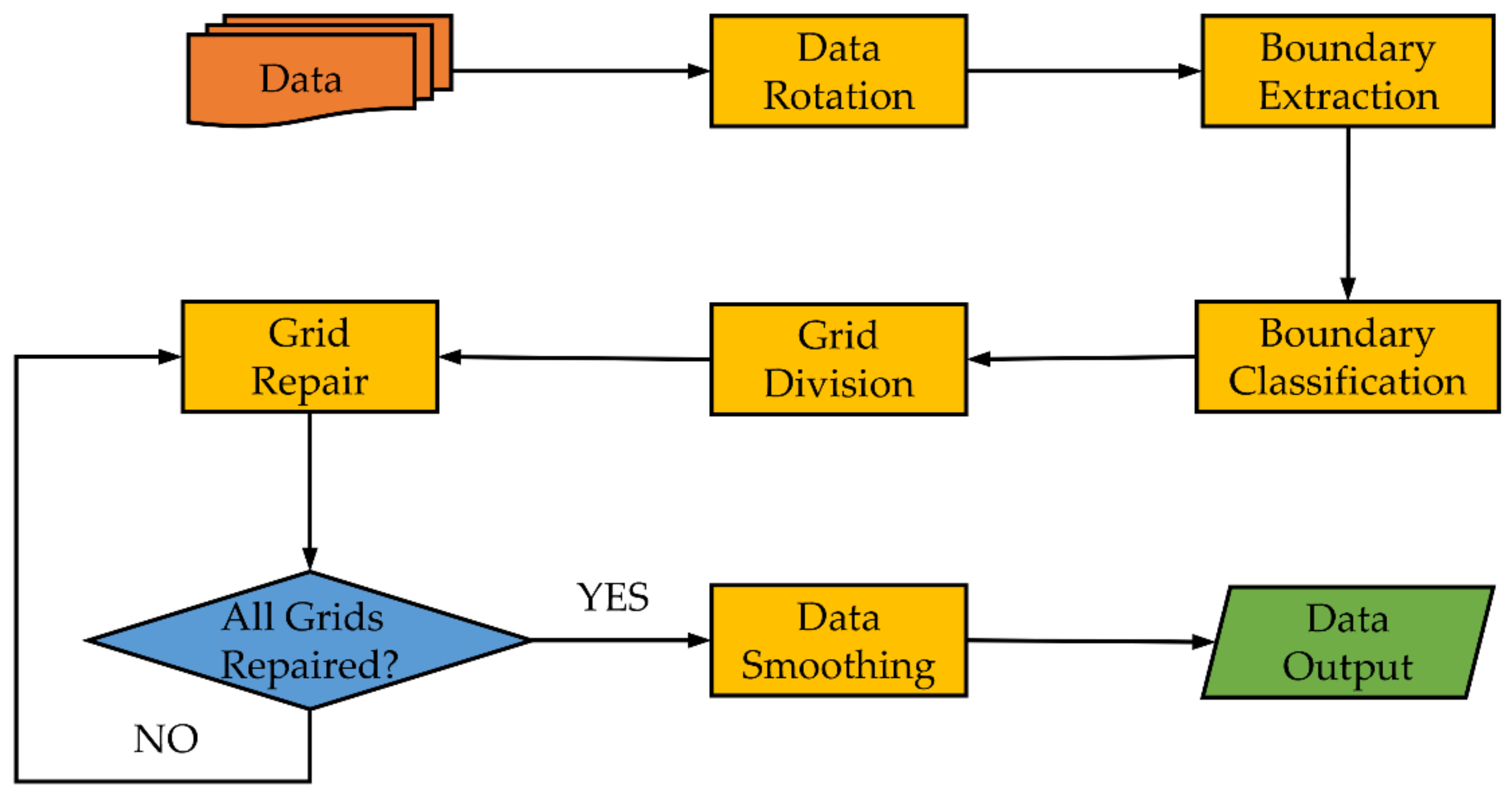
The technical flow chart of the “fuzzy” repair method proposed in this paper is shown in Figure 1. First, we rotated the pre-processed point cloud data to make the facade parallel to the plane XOZ. This step can make subsequent processing more convenient. For example, we only need to consider the X-axis and Z-axis when extracting the boundaries. After that, in the process of boundary extraction, we mainly extracted the feature boundaries representing the building structure (wall, door, and window boundaries). Furthermore, we used the boundary classification method proposed in this paper to divide the feature boundaries into horizontal and vertical feature boundaries. Finally, we carried out grid division and repair according to the extracted boundaries. The division and repair method will be described in detail later. When all grids were repaired, we output the final repair result through point cloud smoothing.
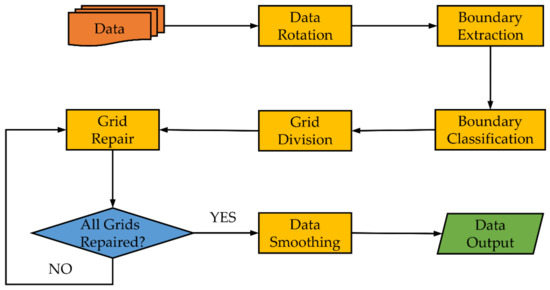
Figure 1.
The technical flow chart of the “fuzzy” repair method.
2.1. Research Data
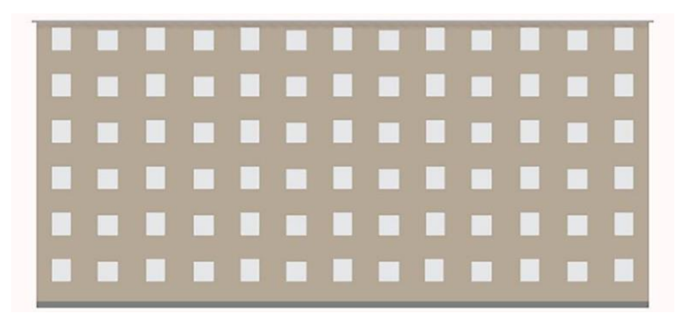
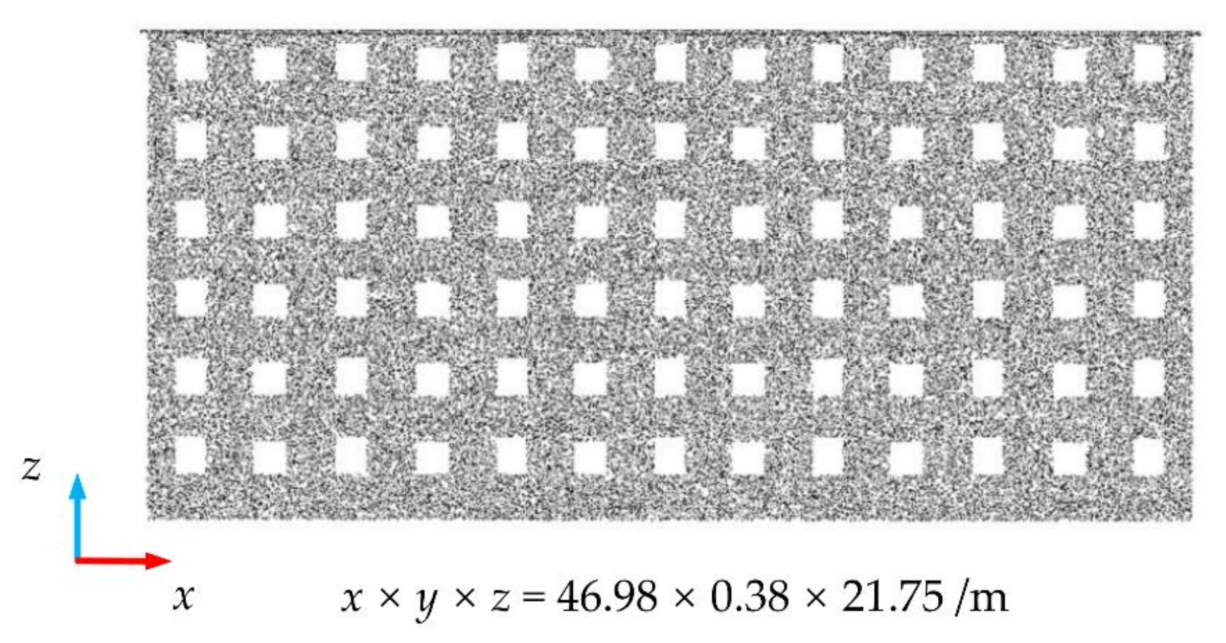
In this research, we used data from four building facades for experiments. Data 1 are the point cloud data converted from the BIM of a teaching building in Shanghai, China; Figure 2 shows the original picture of the BIM; and Figure 3 shows the converted point cloud. The data quality was good, and there were no noise points.
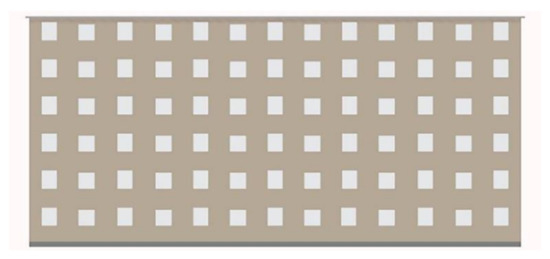
Figure 2.
The BIM of Data 1.
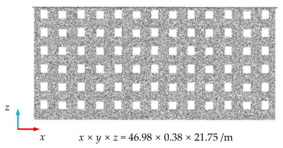
Figure 3.
The converted point cloud of Data 1.
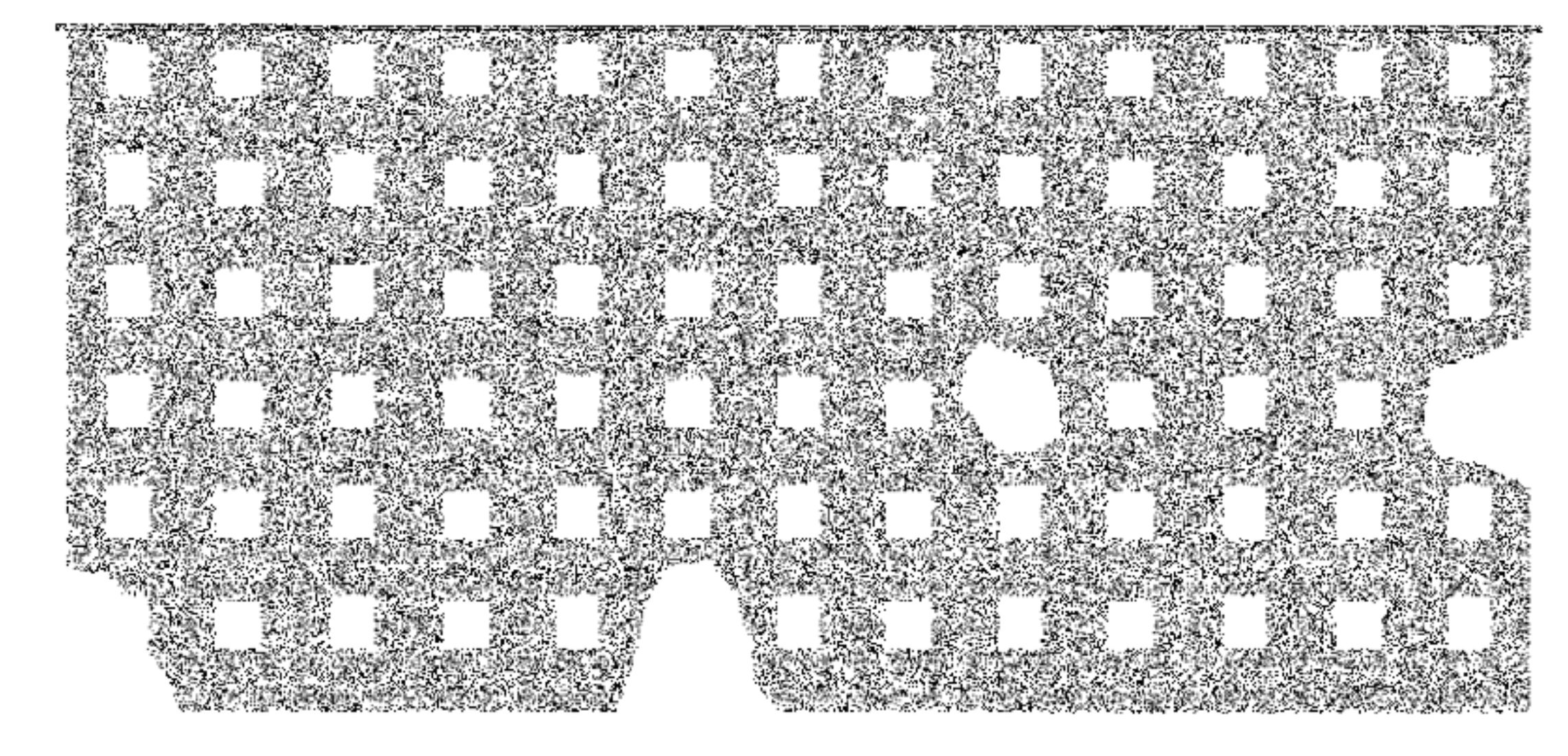
In the follow-up research, we will manually intercept part of the point cloud to obtain holes for the test. There were four holes in the following locations: the lower-left corner, the lower boundary, and the right boundary, as well as an internal hole. A picture of the holes is shown in Figure 4.
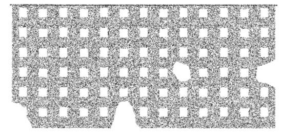
Figure 4.
The manual holes of Data 1.
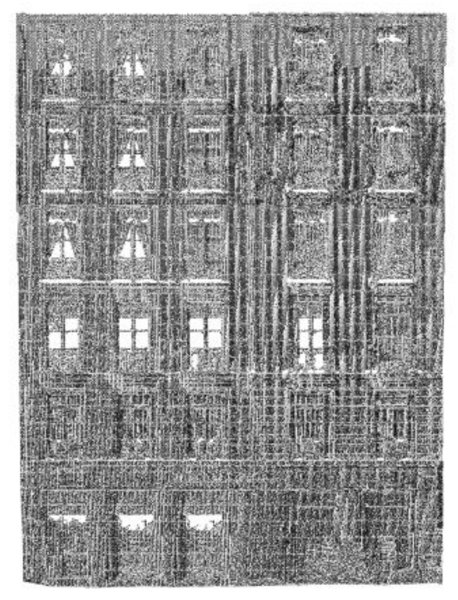
Data 2 and Data 3 are facade point clouds of the building in the Semantic 3D public dataset, with the TLS collected. The point cloud density was relatively high. To reduce the load on the computer, we subsampled them in this study (this step is not necessary). Data 2 and Data 3 are shown after subsampling in Figure 5 and Figure 6, respectively. The loss of the two kinds of point clouds was mainly generated at the bottom, caused by the occlusion of vehicles and flower beds.

Figure 5.
The original diagram of Data 2 (sg28_5 of Semantic 3D data set) after subsample.

Figure 6.
The original diagram of Data 3 (stgallencathedral1 of Semantic 3D data set) after subsample.
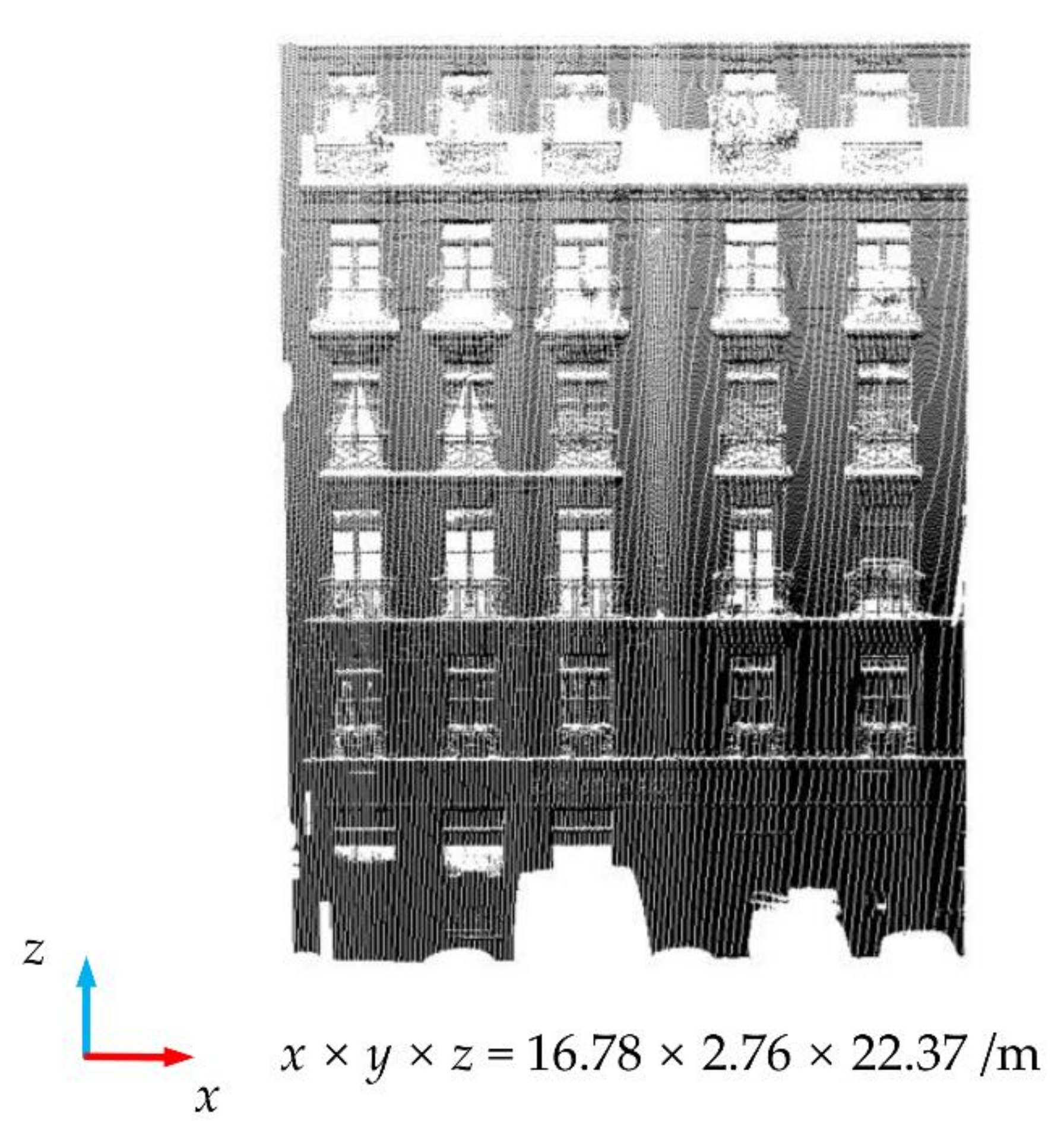
Data 4 [28] shows the point cloud of a building facade cut in a block of Paris, France, of the public dataset of IQmulus & TerraMobilita Contest, which was obtained by a vehicle-borne laser scanner. Due to the angle limitations of the scanner and the occlusion of a car, there is large data loss in the upper and lower areas. A picture of Data 4 [28] is shown in Figure 7.

Figure 7.
The original diagram of Data 4 [28] (the data was obtained from the public data set of the “IQmulus & TerraMobilita Contest”).
The experimental data are shown in Table 1:

Table 1.
The information for the experimental data.
2.2. Point Cloud Rotation
The attitude of the original point cloud is usually arbitrary, and the critical basis of grid-division is to extract the feature boundaries of the point cloud. The point cloud data should be rotated to adjust the attitude to facilitate the subsequent classification of feature boundaries and repair holes. In this study, we made the normal building facade parallel to the Y-axis. The building facade was rotated to be parallel to the plane XOZ.
In the acquisition process of the original point cloud, the laser scanner can usually ensure that the Z-axis of the coordinate system is vertical and upward, only needing to rotate an angle around the Z-axis in the XOY plane [29]. To ensure that the point cloud can be rotated to plane XOZ as much as possible, the PCA [30,31] algorithm was adopted to calculate the main direction on the main facade, and the point cloud was rotated according to this main direction. The main facade refers to the face containing the largest number of points, which is usually a wall and a plane. To obtain this main facade, Random Sample Consensus (RANSAC) [32,33,34] algorithm was used for plane-fitting the point cloud. The RANSAC algorithm can fit the optimal plane in the presence of outliers and then select the plane as the main facade. Once the main direction of the plane is obtained, the rotation matrix can be constructed to rotate it to the plane XOZ. The rotation matrix can be obtained by the Rodriguez rotation formula [35,36], which is expressed as:
where is the rotation matrix. Then, is the angle of rotation and it can be obtained by the cross-product between the main direction of the main facade and the main direction of the plane XOZ. The unit vector of the axis of rotation is .
2.3. Feature Boundaries Extraction
In the process of extracting feature boundaries to build facades, feature boundaries mainly refer to the door, window, and wall boundaries, which are the key to grid-division. The door, window, and wall boundaries are usually represented as endpoints, inflection points, or boundary points on the data. To extract these points, the method based on normal vector estimation [37,38] was adopted to realize the detection and extraction of feature boundaries. The detection and extraction methods are as follows:
- Traverse all points on the data; for the point , search its r-neighborhood points for local feature analysis, and estimate the r-neighborhood normal vector. At this time, if the neighborhood radius r is too small, the noise will be large, and the estimated normal vector is prone to errors. However, if the r is set too large, the estimation speed will be slow. According to the data density, r is generally selected as 0.1–1.0 m. An estimate of the normal vector can be expressed as Formula (2):where M is the covariance matrix. The minimum eigenvalue of M is , and its corresponding eigenvector is the normal vector and . The average value of all points x in the point set is . The average of all points y in the point set is . The average value of all points z in the point set is .
- TLS or MLS are due to errors and environmental reasons in the measurement work will produce outliers of different sparseness levels. Outliers will complicate feature operations such as normal vector estimation or curvature change rate at local point cloud sampling points. This leads to incorrect values, which, in turn, lead to post-processing failures. To solve this problem, we use a method based on distance filtering to remove outliers: calculate the average distance between all points in the r neighbor domain and ; if the distance is greater than , is an outlier point that is removed; otherwise, go to step 3.
- Construct the KD-tree index on the point cloud data, use the angle between each normal direction as the judgment basis, and calculate the normal angle of k neighborhood points. If the included angle is greater than the threshold , it is classified as a boundary feature point. The angle threshold is usually set to or . The smaller the value of the neighborhood point k, the more internal points are identified and the worse the boundary identification accuracy. The larger the value k, the better the accuracy of the final boundary identification. However, if the value k is too large, the boundary points of doors or windows may be ignored. the data from many experiments indicate k usually takes 5–10 times the point spacing Rp.
2.4. Classification of Rectangle Translation
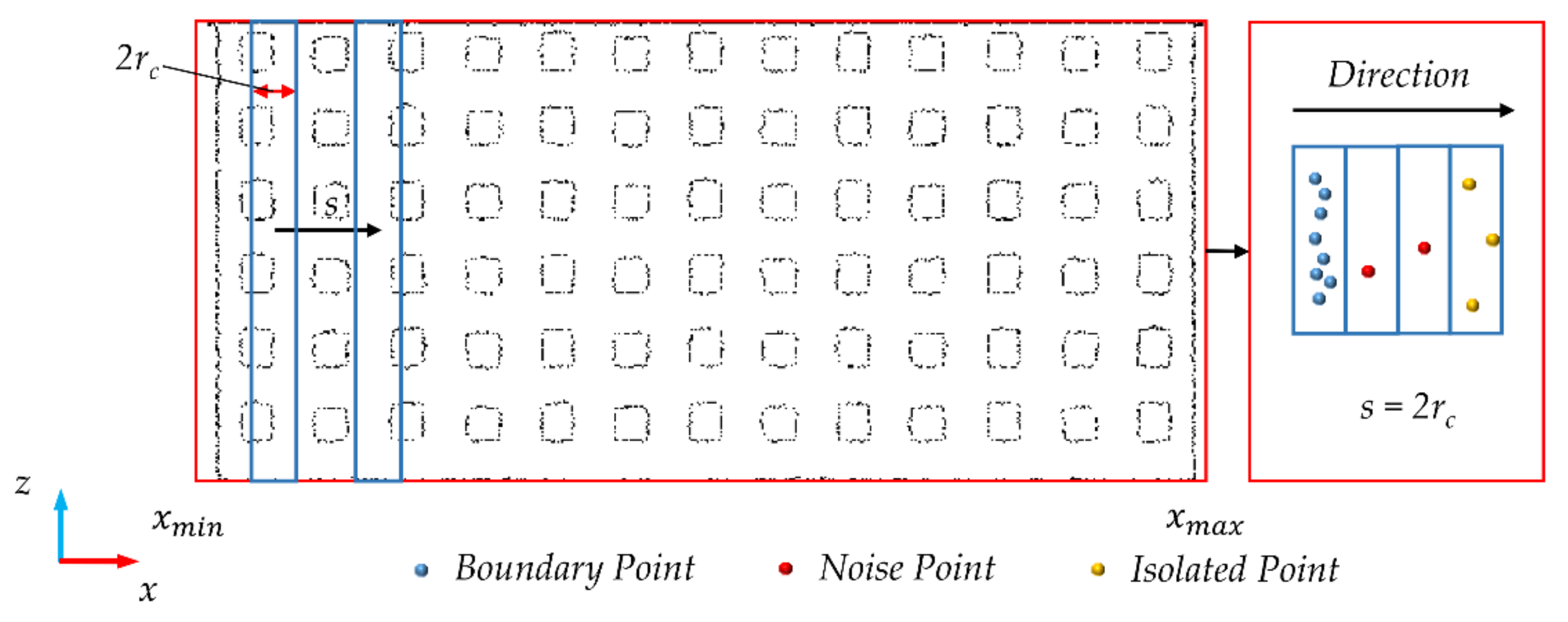
Most of the feature boundaries on the building facade are parallel or perpendicular to the ground. Moreover, after extraction, the point cloud data usually contain noise points and isolated points, which should be filtered out. To divide the point cloud into grids, it is necessary to classify the horizontal and the vertical feature boundaries. In this paper, our classification refers to classifying the extracted feature boundaries as horizontal or vertical. Therefore, we proposed a rectangle translation classification method, which is simple, efficient, and meets the follow-up requirements of this research. This method simulates the translation of a long and narrow rectangle on the data plane and divides the points into clusters by setting the number of points contained in the rectangle. This method can filter noise points and outliers at the same time. The classification method is as follows:
- Project the feature boundaries to XOZ plane;
- Set the Rectangle radius and the translation step size s (generally, step size s is set to 2). When the vertical feature boundaries are extracted, the Rectangle height is the Z-axis length of the point cloud after the boundary extraction. At this time, the Rectangle is translated from to , traversing all the data. If the number of points in the Rectangle is less than the threshold value , these points are discarded. If is greater than , these points are saved. The saved points are all the required vertical feature boundaries;
- The process of extracting horizontal feature boundaries is similar to step 2. In this case, the height of the Rectangle is the X-axis length of the point cloud after the boundary extraction. The Rectangle is translated to from to traverse the entire data.
This method can affect the width of the extracted boundaries by modifying the Rectangle radius and step size s, and effectively removing noise points and outlier points. The translation diagram is shown in Figure 8. In the figure, the blue is the created rectangle. The rectangle moves from xmin to xmax, and each translation distance is s. The blue points are reserved feature boundary points, red points are noise points, and yellow points are isolated points.
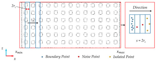
Figure 8.
The schematic diagram of “Rectangle Translation”.
2.5. Grid Division and Repair Based on Distribution Regularity
The “fuzzy” repair method proposed in this paper is a “copy–paste” method based on grids. This section will explain the basis and method of grid-division and the principle of repairing point cloud holes.
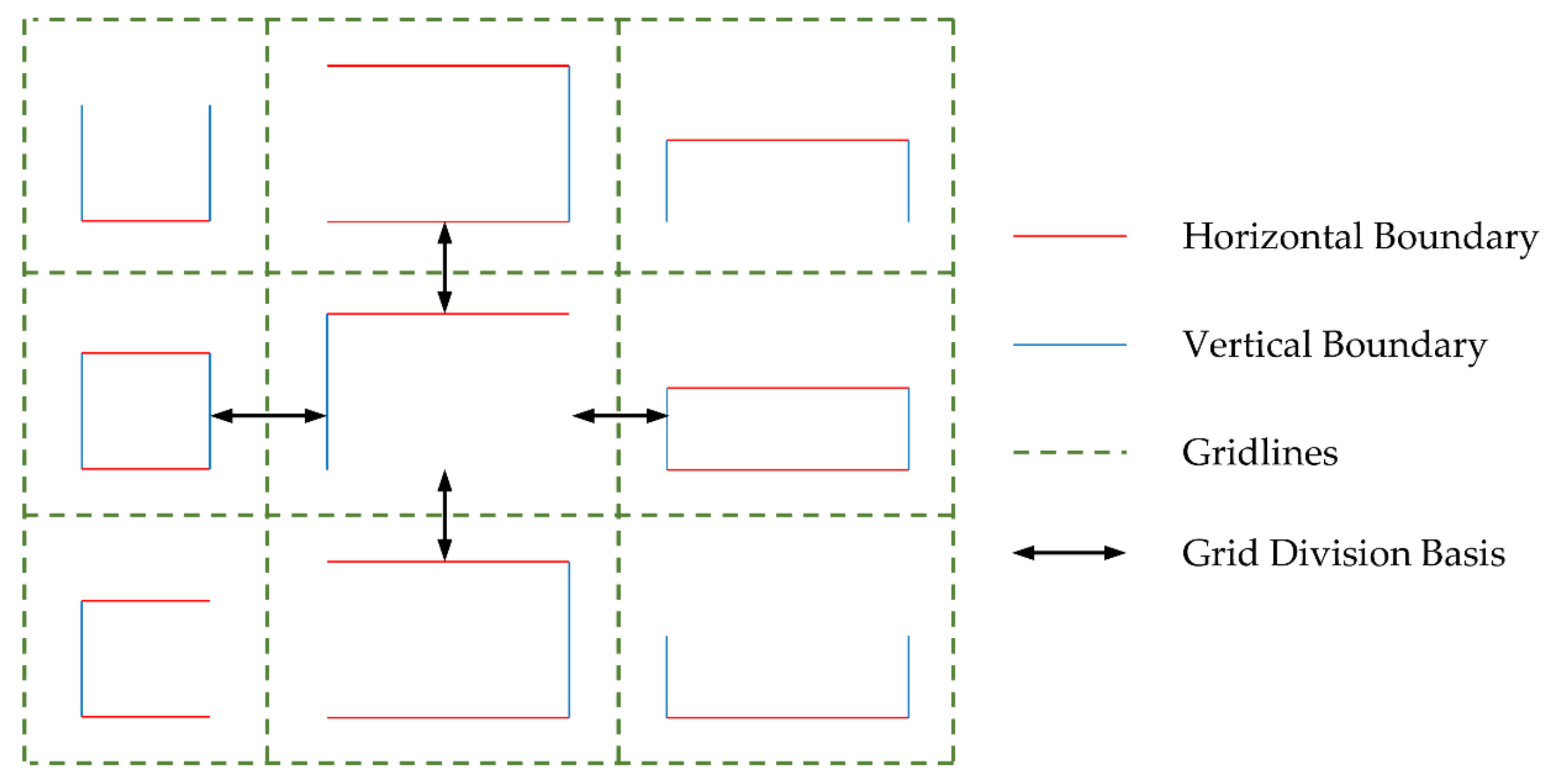
In the process of hole repair, considering the distribution regularity of buildings, to ensure that each window or door can be preserved as much as possible, we try to use each window or door as a grid, and the grid-division should comply with the following principles:
- In the horizontal direction, the two adjacent grids are based on the boundary of two adjacent windows (doors) on the left and on the right, and half of the boundary distance between the two adjacent windows (doors) is taken as the division;
- In the vertical direction, as in Step 1, we take half of the boundary distance between the upper and the lower adjacent windows (doors) for division;
- When a window (door) does not extract the feature boundaries during boundary extraction, the division is based on the other window (door) boundaries in the same row or column;
- When there are two windows (doors) of different sizes in a row or a column, the division is carried out according to the boundary of the larger window (door).
The grid-division principle can be represented as Figure 9:
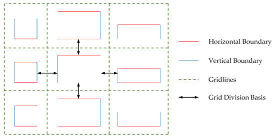
Figure 9.
The diagram of grid-division principle.
As shown in Figure 8, when the boundaries of a window are not extracted, as long as there are other feature boundaries in the row or column, the grid-division of the window can also be carried out. Therefore, the “fuzzy” point cloud repair method does not need to be particularly strict in extracting the feature boundaries of the original data, and it is suitable for data whose boundaries are difficult to extract.
When dividing the grids, we divide windows into three types: internal, boundary, and corner windows (only boundary doors exist). The method of grid-division is shown as follows:
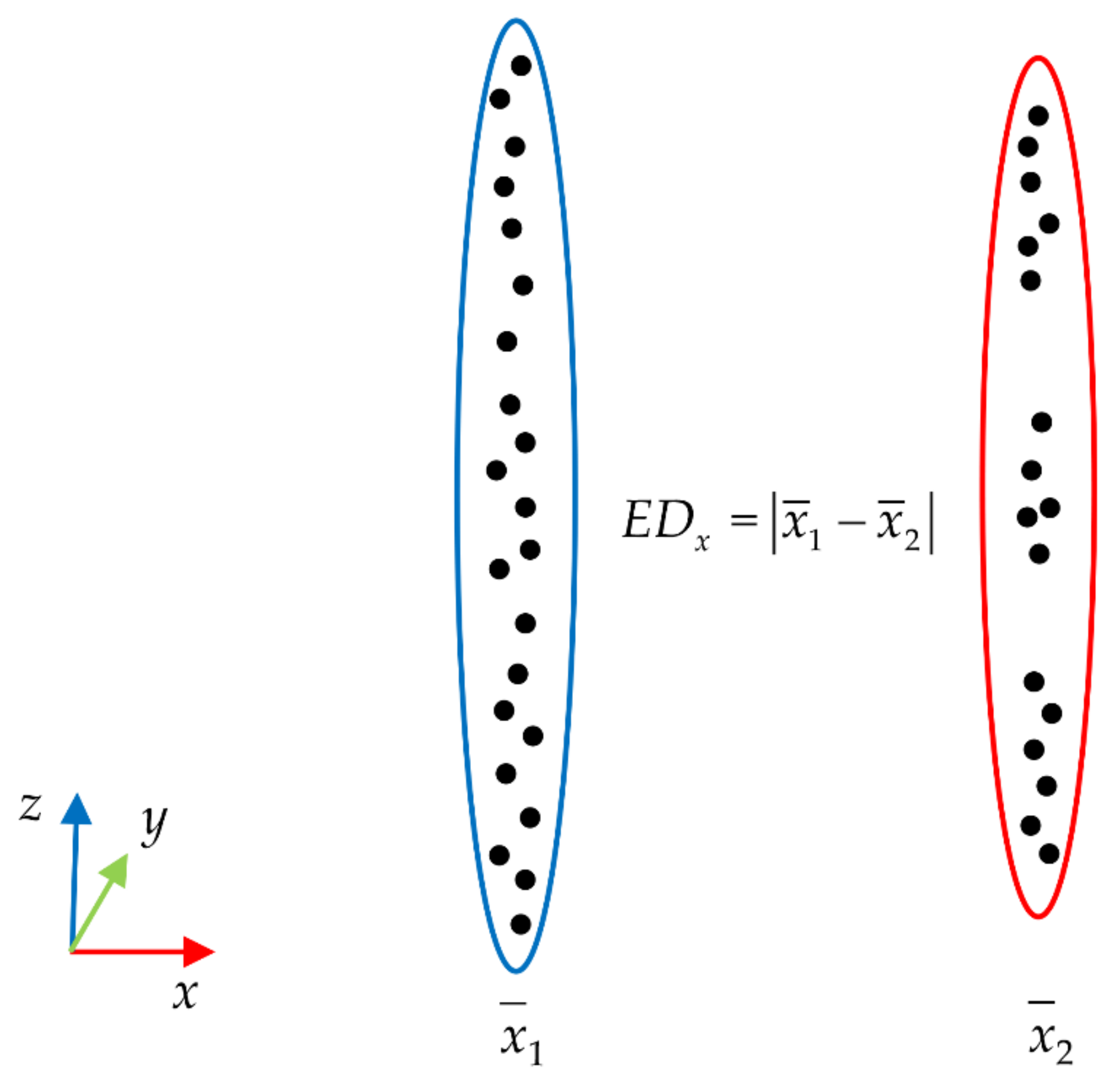
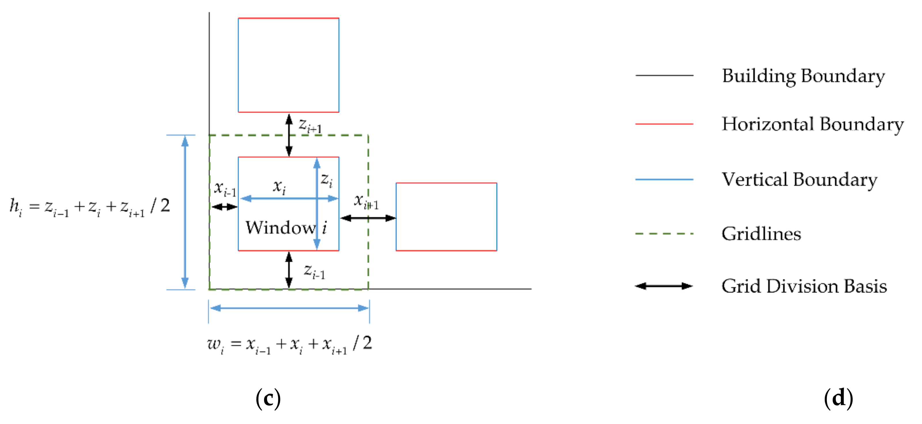
- When dividing the grids, we divide windows into three types: internal, boundary, and corner windows (only boundary doors exist). The method of grid-division is shown as follows: After obtaining the horizontal and vertical feature boundaries of buildings in Section 2.4, the Euclidean distance is used to calculate the distance of two adjacent boundaries as , . As shown in Figure 10, the Euclidean distance refers to the difference between the average values of the X-axis (Z-axis) of two adjacent feature boundary point clouds;
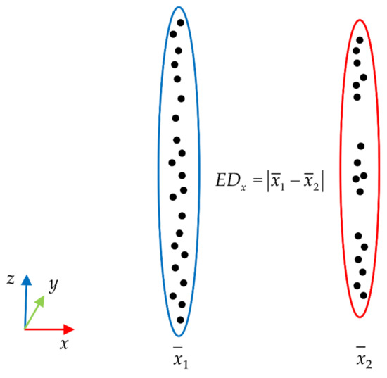 Figure 10. The calculation method of Euclidean distance.
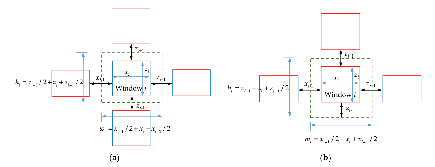
 - When i is an internal window, set its width to and height to . If the distance between it and the window (i − 1) is and the distance between it and window (i + 1) is , then the grid width w is . The grid height h of the window is the same as this, which is ;
- When i is the upper or lower boundary window, its width is set to , its height to , and its grid width w to . If the distance between i and the bottom of the building is , and the distance between i and the upper window is , then the grid height h of i is . When i is the left or right boundary window, the grid-division is similar to the upper and lower boundary windows, with the grid width w is , and the grid height h is ;
- When i is a corner window, its width is set to and its height, to . If the distance between it and the bottom of the building is , the distance between it and the upper window is , the distance between it and the left boundary of the building is , and the distance between it and the right window (door) is . Then, the grid width w is , and the grid height h is .
The method of grid division is shown in Figure 11:
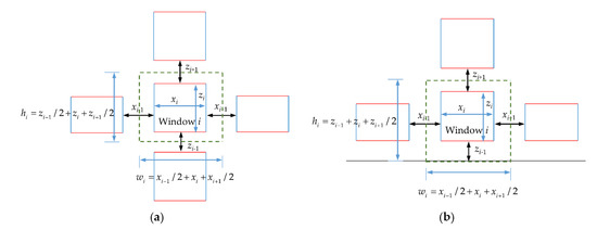
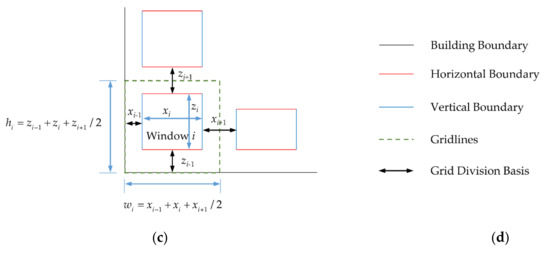
Figure 11.
The diagram of grid-division method: (a) The grid-division method of internal window; (b) The grid-division method of boundary window; (c) The grid-division method of corner window; (d) The legend of grid-division diagram.
In this paper, we proposed a repair principle and method that conforms to the distribution regularity of buildings. The principle and method can be described as follows:
- Define the threshold of the number of points in the grid to determine whether the grid is to be repaired. The definition of is not fixed. Considering that the number of point clouds in the occluded area is usually significantly lower than that in the unoccluded area, can be set according to the point density of all grids. Generally speaking, the setting of is as follows:where is the total number of points in grid i. The grid volume i is . The total number of grids is n.
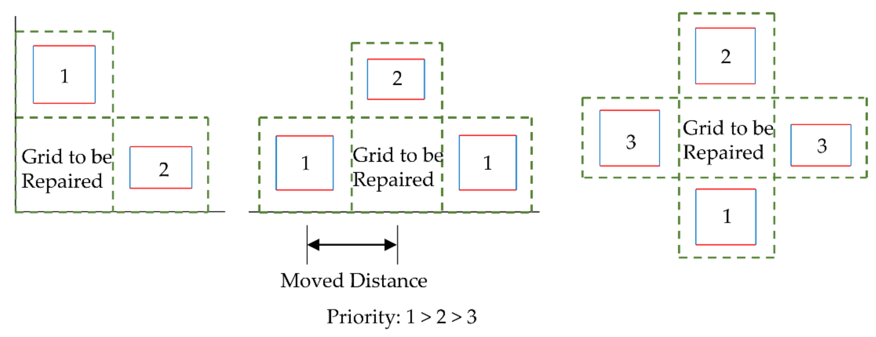
- When the internal grid is to be repaired, adjacent columns will first be selected to repair the internal grid due to the similar structural feature of the columns. At this time, considering the characteristics of laser scanners, the density of low-elevation point clouds is usually denser than that of high-elevation point clouds. Therefore, the lower adjacent columns are first selected to repair the grid, and the upper adjacent columns are selected second. When both the upper and the lower adjacent columns are to be repaired, the left and the right adjacent rows are selected to repair the grid. When all four adjacent grids are to be repaired, the grid will be temporarily shelved and repaired in the next cycle until all the grids are repaired;
- When the boundary grid is to be repaired, for the upper and lower boundary grids, the height is different from that of the internal grid because one side is close to the wall but similar to the adjacent boundary grids. Therefore, the adjacent boundary grids are first selected for repair. When the adjacent boundary grids are both to be repaired, the adjacent internal grids are selected for repair. When all the adjacent boundary grids and internal grids are to be repaired, the grid will be temporarily shelved and repaired in the next cycle until the repair of all grids is complete. The repair principle of left or right boundary grids is similar;
- When the corner grid is to be repaired, the width of the grid is usually different from the width of the upper and lower boundary grids, and the height of the grid is different from the length of the left and the right boundary grids because the two sides of the grid are close to the wall. This kind of grid repair is difficult. Therefore, we try to carry out a “copy–paste” repair from the column to the grid, as the features of the door and the window in the column are usually similar or the same in most buildings, while the features in the row may be quite different. When the adjacent column grid is also the grid to be repaired, the adjacent row grid will be selected for repair. When all the adjacent column and row grids are to be repaired, the grid will be temporarily shelved and repaired in the next cycle until all grids are repaired;
- After the point cloud repair principle is determined, for the grid to be repaired, we delete all points in the grid, copy all points in the adjacent grid, and fill these points into this grid. Finally, the repair of holes in the point cloud is realized through point cloud smoothing. Therefore, this method can also be regarded as a “copy–paste” repair method. Here, since the point cloud has been rotated to be parallel to the XOZ plane, when performing “copy–paste”, we need only to change the coordinates on a particular axis to complete the “paste”.
The grid repair principle can be expressed as in Figure 12. As shown in the figure, to “copy–paste” the point cloud in the left grid into the right grid, we need only to change the X-axis coordinates of all points in the left grid, and the distance moved is the distance between the centers of the two grids, which can be obtained from the grid size. In summary, to make the point cloud information correct after the “paste”, point cloud rotation is essential.
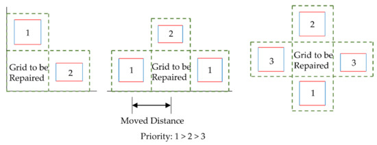
Figure 12.
The diagram of grid repair principle.
2.6. Evaluation Indicators
To quantify the point cloud repair accuracy and efficiency of the algorithm in this paper, we used the manual repair result as a comparison standard, which was considered the most precise method in the literature [39] (for Data 1, we used the converted point cloud data as the standard data) and proposed two evaluation indicators of point cloud integrity (Pintegrity) and compatibility (or precision, Pcompatibility). Among them, the manual repair result was realized by combining the software of Point Cloud Magic (PCM) and Geomagic Studio. First, we used PCM to preprocess the point cloud (point cloud segmentation, subsample, denoising, etc.) and then we used the Geomagic Studio (based on the Delaunay triangle grid method) to repair the three experimental data, and the repair time was recorded. The integrity of the point cloud represents the ratio of the total number of point clouds before (after) “fuzzy” repair to the total number of point clouds after manual repair. The compatibility of point cloud represents the average value of included angle (Pangel) and the Y-axis position deviation average (Pposition) between the largest principal plane of the point cloud in the repaired grid and the largest principal plane of the point cloud in the adjacent n (n = 2, 3, 4) grids. The calculation formula for integrity and compatibility is:
where is the total number of the initial point cloud, is the total number of point cloud after the “fuzzy” repair, and is the total number of the point cloud after the manual repair. The normal vector of the largest principal plane of the point cloud in the repaired grid is , and is the normal vector of the largest principal plane of the point cloud in the adjacent grid i. The Y-axis coordinate of the center point of the largest principal plane of the point cloud in the repaired grid is , and is the Y-axis coordinate of the center point of the largest principal plane of the point cloud in the adjacent grid i.
3. Results
3.1. Point Cloud Rotation Results
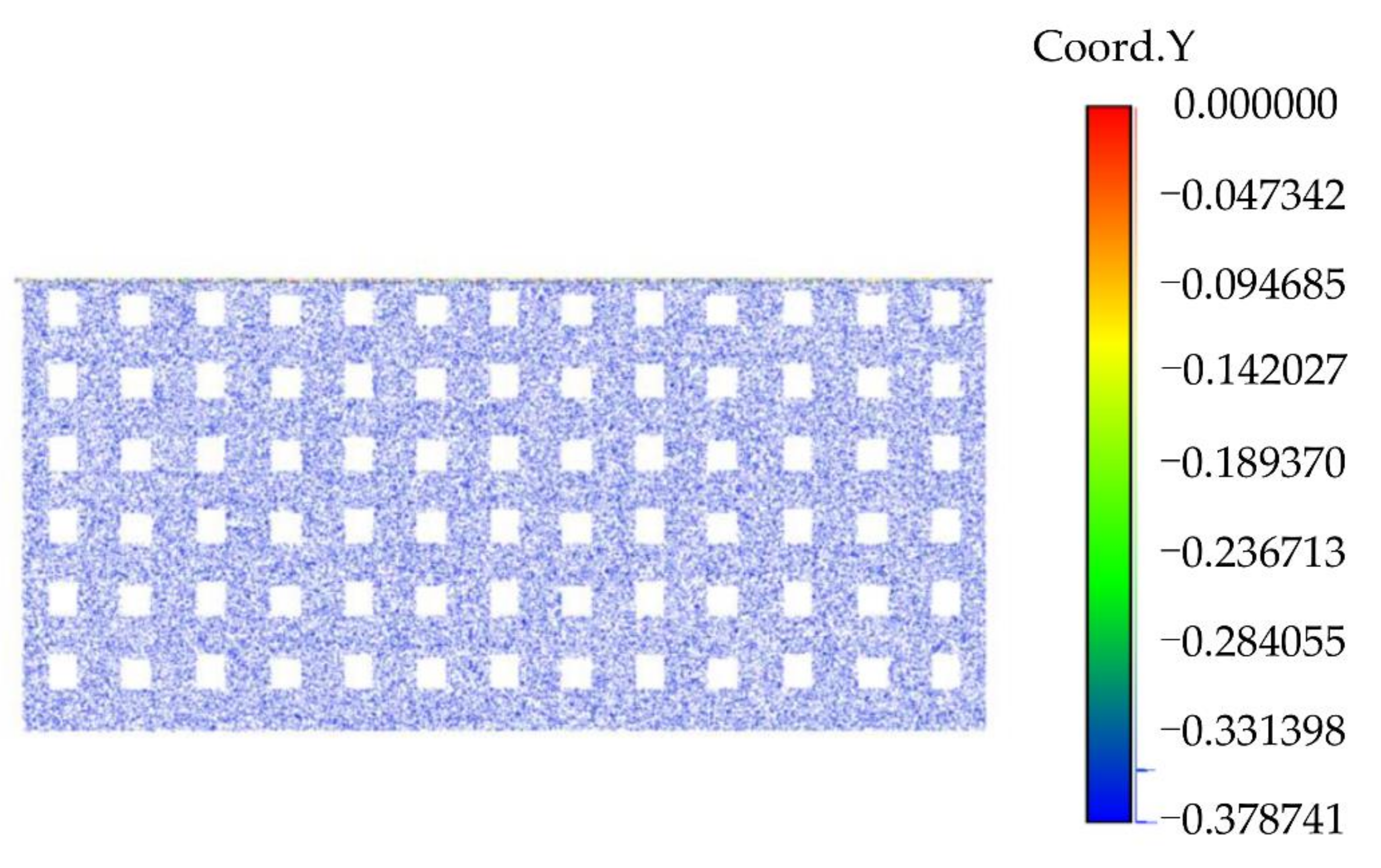
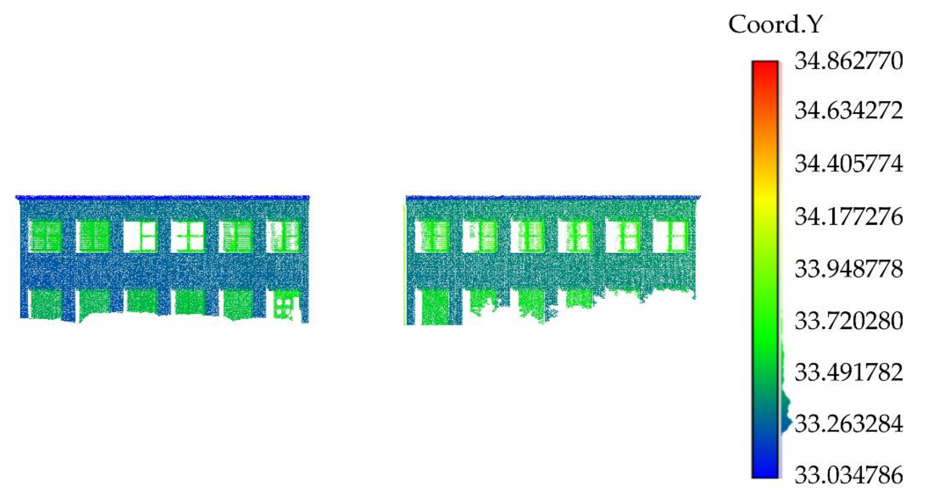
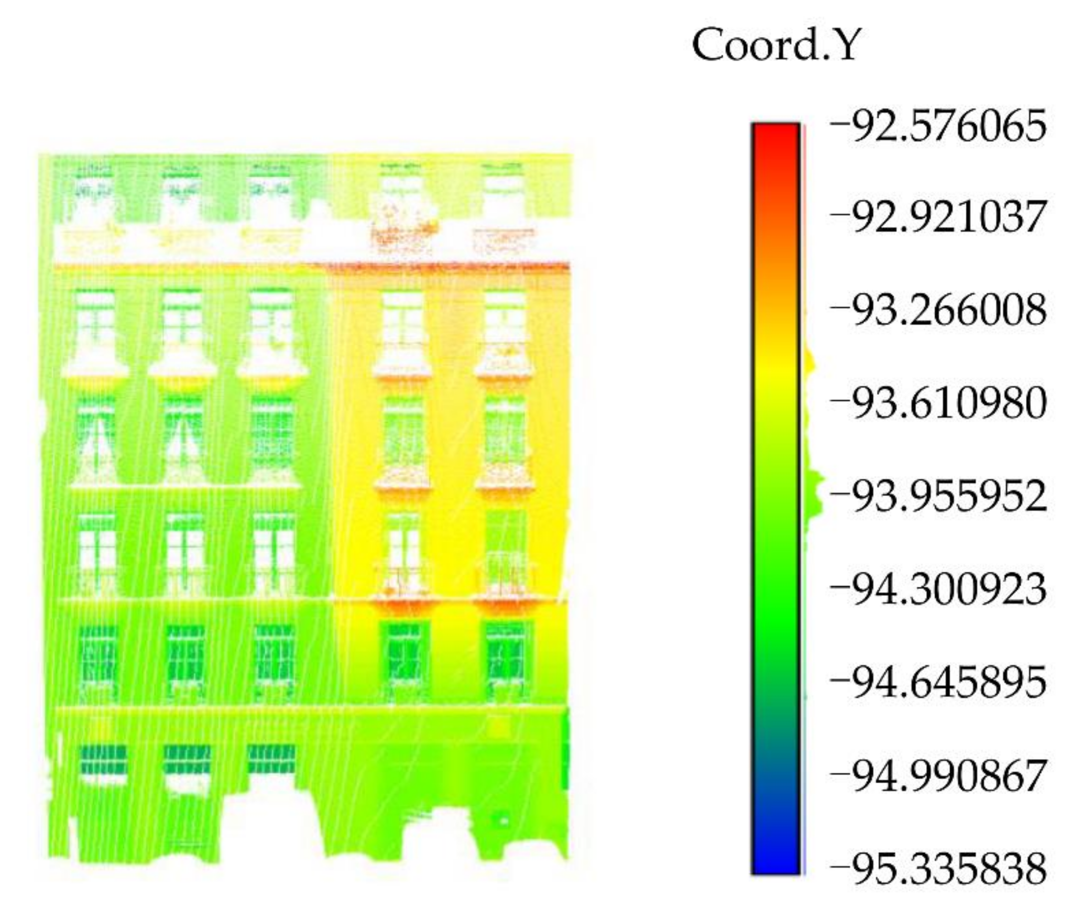
The point cloud rotation results of Data 1, Data 2, Data 3, and Data 4 [28] are shown in Figure 13, Figure 14, Figure 15, and Figure 16, respectively. It can be seen from the scalar field diagram on the Y-axis that the point cloud rotation results meet the requirements of subsequent experiments.
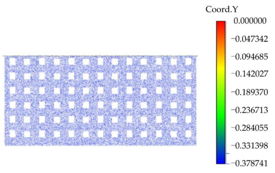
Figure 13.
The scalar field of Data 1 on the Y-axis.

Figure 14.
The scalar field of Data 2 on the Y-axis.
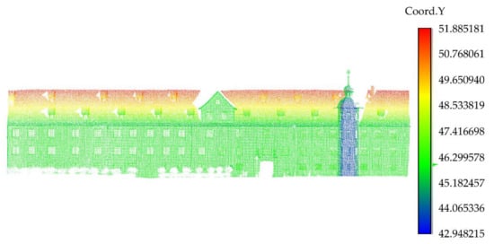
Figure 15.
The scalar field of Data 3 on the Y-axis.

Figure 16.
The scalar field of Data 4 [28] on the Y-axis (the original data was obtained from the public data set of the “IQmulus & TerraMobilita Contest”).
3.2. Feature Boundaries Extraction Results
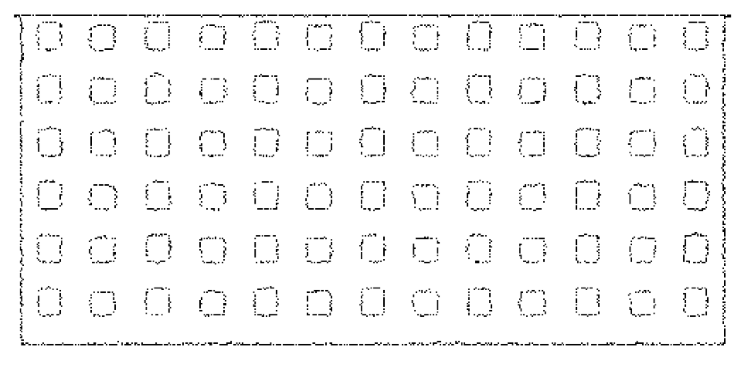
The feature boundaries’ extraction results of Data 1, Data 2, Data 3, and Data 4 [28] are shown in Figure 17, Figure 18, Figure 19, and Figure 20, respectively. Figure 21 is the RGB point cloud diagram of Data 3:
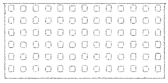
Figure 17.
The boundary extraction results of Data 1.

Figure 18.
The boundary extraction results of Data 2.

Figure 19.
The boundary extraction results of Data 3.
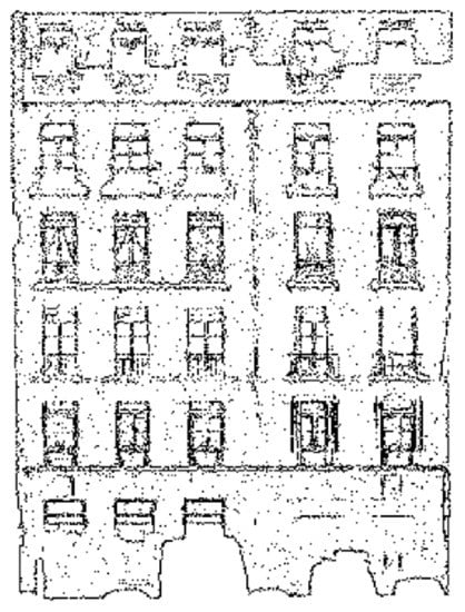
Figure 20.
The boundary extraction results of Data 4 [28] (the original data was obtained from the public data set of the “IQmulus & TerraMobilita Contest”).

Figure 21.
The RGB point cloud diagram of Data 3.
3.3. Rectangle Translation Classification Results
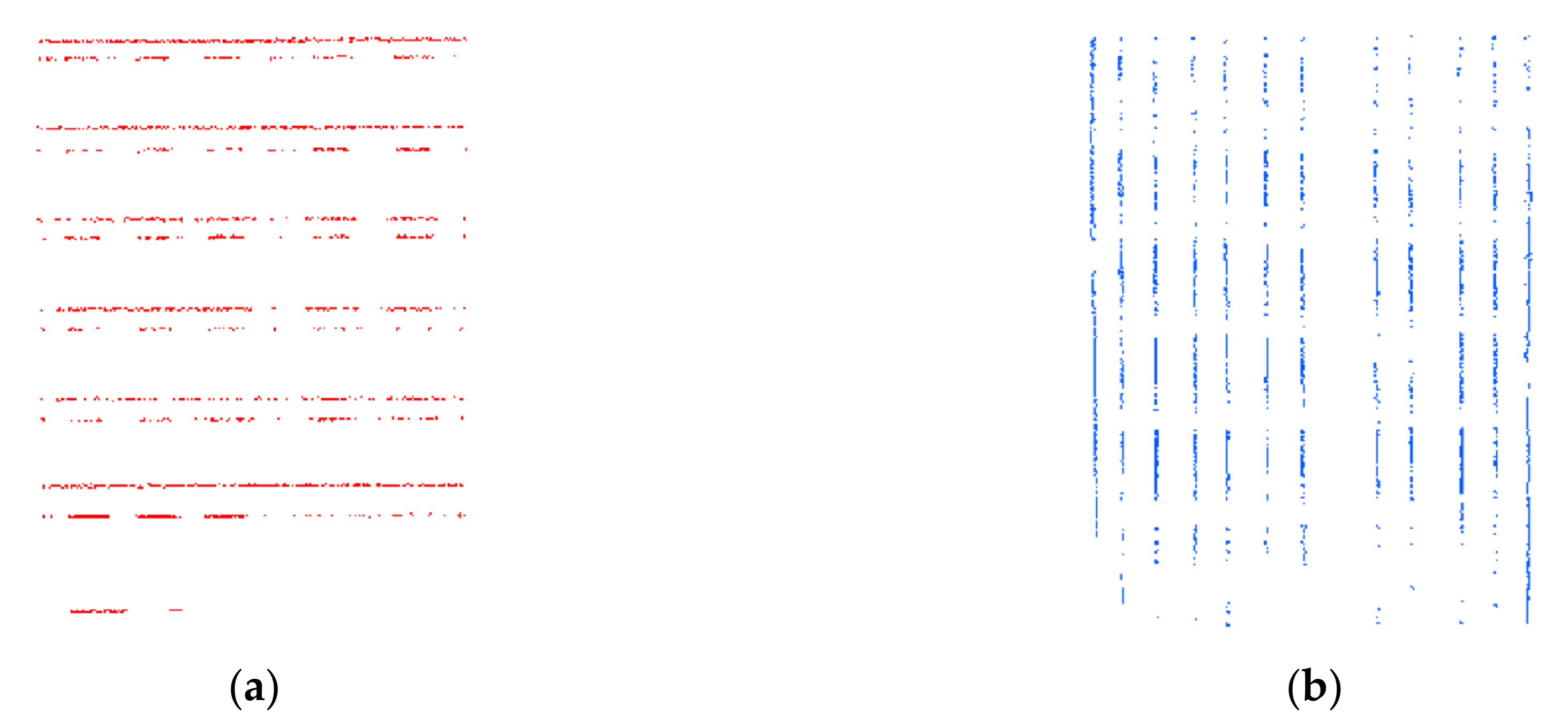
The Rectangle Translation classification results of Data 1, Data 2, Data3, and Data 4 [28] are shown in Figure 22, Figure 23, Figure 24, and Figure 25, respectively:

Figure 22.
The classification result of Data 1: (a) The horizontal feature boundaries’ extraction results of Data 1; (b) The vertical feature boundaries’ extraction results of Data 1.

Figure 23.
The classification result of Data 2: (a) The horizontal feature boundaries’ extraction results of Data 2; (b) The vertical feature boundaries’ extraction results of Data 2.

Figure 24.
The classification result of Data 3: (a) The horizontal feature boundaries’ extraction results of Data 3; (b) The vertical feature boundaries’ extraction results of Data 3.
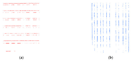
Figure 25.
The classification result of Data 4 [28] (the original data was obtained from the public data set of the “IQmulus & TerraMobilita Contest”): (a) The horizontal feature boundaries’ extraction results of Data 4 [28]; (b) The vertical feature boundaries’ extraction results of Data 4 [28].
3.4. Point Cloud Repair Results
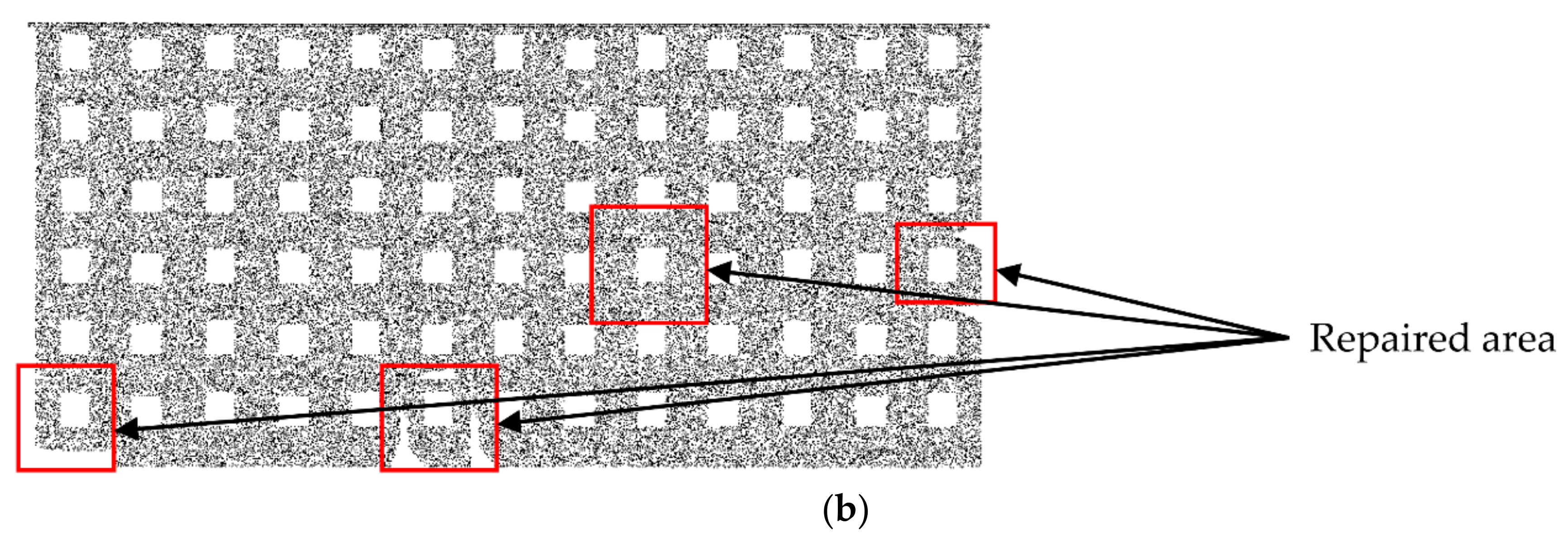
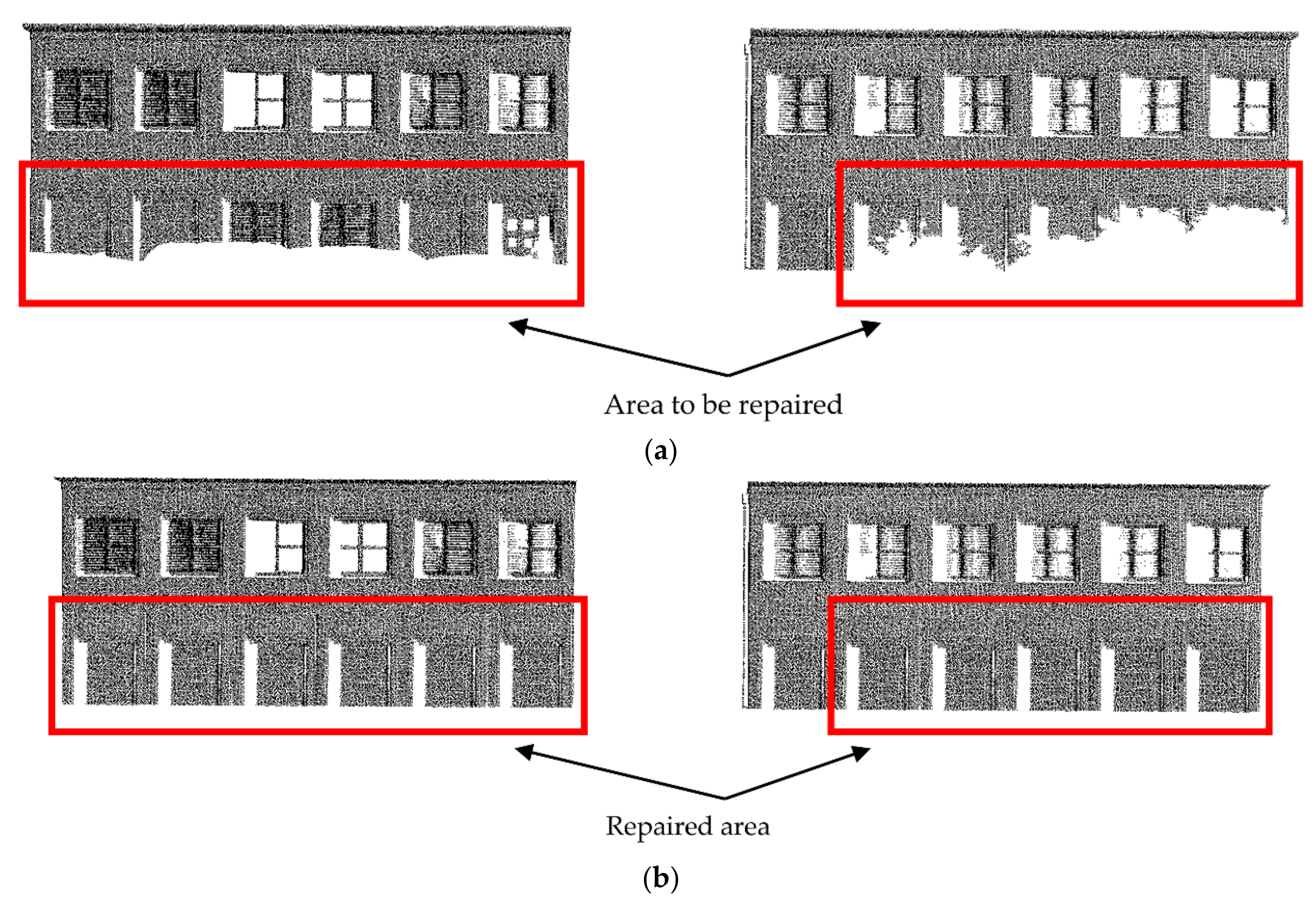
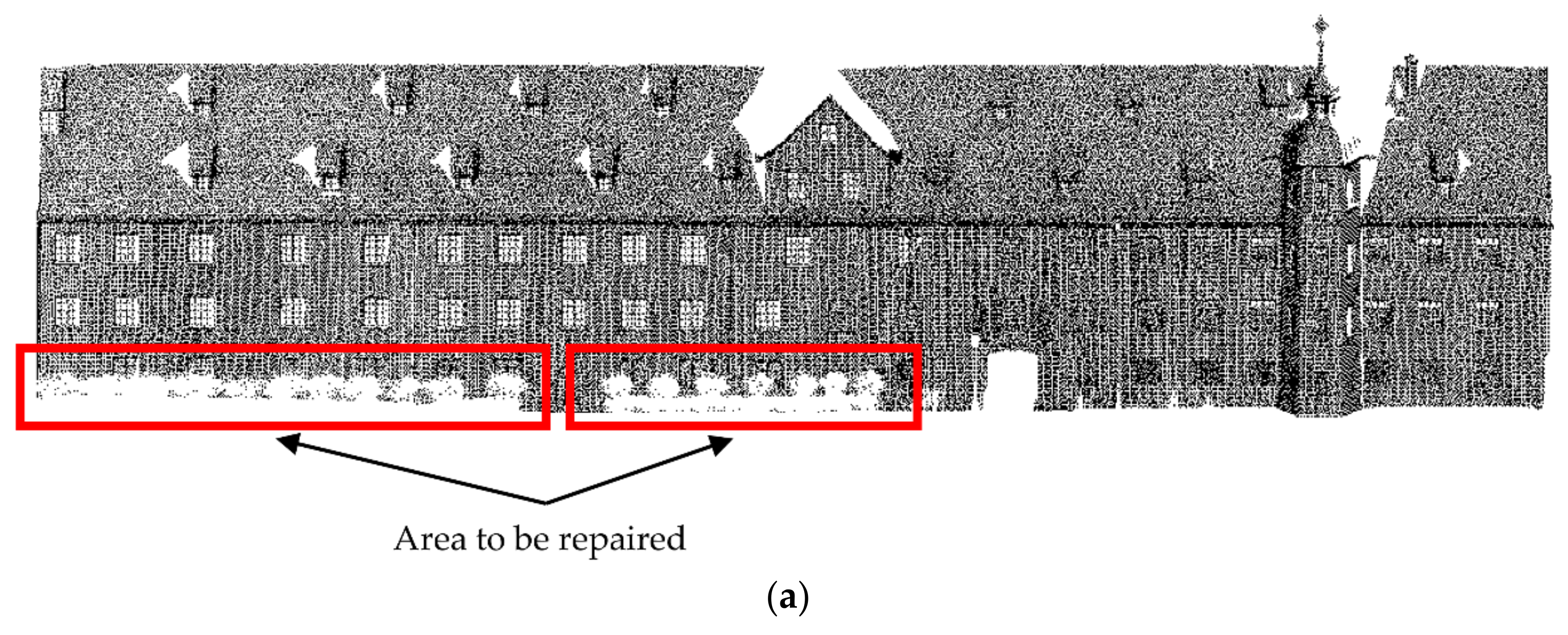
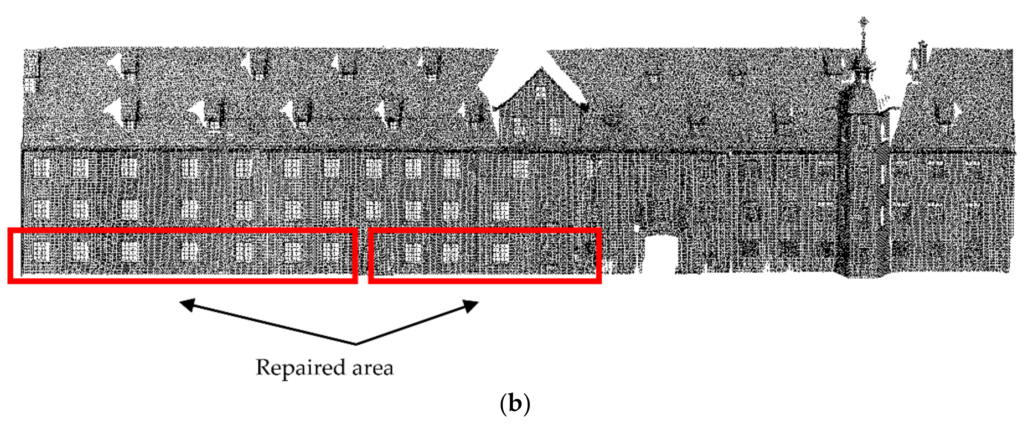
The comparison results of the point cloud before and after the repair of Data 1, Data 2, Data 3, and Data 4 [28] are shown in Figure 26, Figure 27, Figure 28, and Figure 29, respectively:


Figure 26.
The repair results of Data 1: (a) Before repair; (b) After repair.
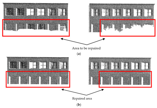
Figure 27.
The repair results of Data 2: (a) Before repair; (b) After repair.
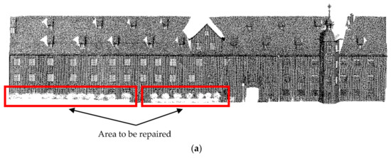
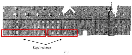
Figure 28.
The repair results of Data 3: (a) Before repair; (b) After repair.
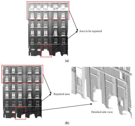
Figure 29.
The repair results of Data 4 [28] (the original data was obtained from the public data set of the “IQmulus & TerraMobilita Contest”): (a) Before repair; (b) After repair.
The selection and the basis of each parameter in the repair process are shown in Table 2.

Table 2.
The selection and basis of each threshold.
According to Equations (4)–(6), and Table 1, the integrity and compatibility of the four experimental data are calculated. The calculation results are shown in Table 3 and Table 4, respectively.

Table 3.
The calculation results for integrity.

Table 4.
The calculation results for compatibility.
The manual repair results of Data2, Data3, and Data4 are shown in Figure 30, Figure 31 and Figure 32:

Figure 30.
The manual repair results of Data 2.

Figure 31.
The manual repair results of Data 3.

Figure 32.
The manual repair results of Data 4 [28] (the original data was obtained from the public data set of the “IQmulus & TerraMobilita Contest”).
To compare the efficiency of the algorithm in this paper, we listed the time of manual repair (repair method based on Delaunay triangle grid) and the time of the “fuzzy” repair algorithm proposed in this paper. The two repair methods were running in the same environment: Intel(R) Core(TM) i7-7700HQ CPU @ 2.80 GHz, the memory was 32 G, and the graphics card was an NVIDIA GeForce GTX 1060. The time comparison is shown in Table 5:

Table 5.
The time comparison of “fuzzy” and manual repair.
4. Discussion
4.1. The Discussion of Feature Boundaries Extraction Results
For Data 2, the boundary extraction result is better (as shown in Figure 18). In Data 3, comparing the windows in the red frame of the RGB data (as shown in Figure 21), it can be seen that the extraction result of the windows on the right side of the building is poor, and some window boundaries are not extracted at all (as shown in Figure 19). This is because the point cloud of this area is dense, and the normal estimation method cannot distinguish the window and the wall. However, this does not affect subsequent grid-division and point cloud repair because the available feature boundaries are extracted from the same row or column of these windows. Our method is also suitable for such a “fuzzy” extraction result.
For Data 4 [28], some upper window boundaries are also not extracted, and there are many internal points in the result (as shown in Figure 20). This is because the data are relatively denser than Data 1, Data 2, and Data 3, so many internal points are also saved. As mentioned in Section 2.3, for the selection of k neighborhood points, the smaller the value of k, the more internal points will be saved and the worse the boundary identification result. However, the increase in k will lead to the loss of more door or window boundaries, so, we have to retain these internal points but these points will be filtered after “Rectangle Translation”.
4.2. The Discussion of Point Cloud Repair Results
For Data 1, it can be seen that the internal grid has the best repair result, the boundary grid has the second-best repair result, and the corner grid has the worst repair result, but these results are acceptable (as shown in Figure 26). This is because we set the threshold to be small, that is to say, we only repaired the four main holes. Looking at the small holes in the grid, we believe these holes will not greatly impact the whole building, so these grids are not regarded as grids requiring repair.
As can be seen from Figure 26, Figure 27, Figure 28and Figure 29, the repair results of the four pieces of data try to repair the original state of the holes. For Data 2, the lower data are missing, and there is only one complete door (as shown in Figure 27). When repairing Data 2, we replaced the missing data with this door, and the data repair result was acceptable. For Data 3, the lower data are also missing but, differing from Data 2, these missing data are relatively few and they are caused by low grass and flower beds. The missing data contain windows, and missing doors should not be processed. Therefore, we replaced the grid of the missing windows with the grid of the previous row, and the final repair result was in line with expectations (as shown in Figure 28). For Data 4 [28], we tried our best to repair the loss in the upper and lower areas. It can be seen that the upper area of the point cloud is missing due to the angle limitations of the scanner, but since the feature boundaries of this area can be extracted, our method can still repair this area (as shown in Figure 29).
From the results of the four experimental data, it can be seen that the “fuzzy” repair algorithm in this paper is suitable for point cloud data with different densities (average point spacing). Figure 28a has a higher point cloud density (average point spacing is 3.56 cm) and the cloud density of Figure 29a is small (average point spacing is 10.12 cm). Compared with the manual repair results, it can be seen that the point cloud is effectively repaired after using our method, which proves that our method has a certain degree of universality.
Analyzing Table 3 and Table 4, it can be seen that, when the manual repair results are used as the standard, the “fuzzy” repair algorithm in this paper can effectively improve the integrity of the point cloud. The integrity of the four pieces of data increased by approximately 5.78% on average, which proves that our algorithm can effectively repair the point cloud. It can be seen from Table 4 that, for the four experimental data, our method repaired 4, 12, 11, and 11 grids, respectively. The average angle deviations of each repaired grid from the adjacent n grids were, respectively, no greater than 0.21°, 0.36°, 0.54°, and 0.28°. The average position deviation was not greater than 0.05 cm, 2.31 cm, 0.82 cm, and 3.25 cm, respectively. This proves that our repair method has a high enough accuracy. That is, the repaired grid fits the adjacent grid well enough. There were four extremely large outliers in Data 4 [28]. As shown in Figure 17, the upper-right area of Data 4 [28] has a large Y-axis deviation (about 50 cm) compared with other areas. We call this area the deviation area, and this deviation exists when the data are collected. These deviations may be due to scanner errors or structural features of the building itself. Therefore, when calculating the position deviation of the grid in this area, since its adjacent grids may be located in the non-deviation area, this will lead to huge outliers in the final calculation result. These outliers are caused by the original data rather than our method. Such deviations cannot be corrected by our method and they should be corrected in the pre-processing. Therefore, we removed the four outliers to avoid influencing the evaluation indicators.
Analysis of Table 5 shows that, under the same running environment, the repair time of our method was much shorter for the three pieces of experimental data than the manual repair time. In terms of time consumption, the overall efficiency of the “fuzzy” repair algorithm is higher.
In general, when repairing the point cloud holes in the building facade, our method makes the repair results more humane when it is difficult to obtain multi-source data. The quantitative results show that our repair method improved the integrity of the point cloud by an average of about 5.78%. The repaired grid fits well with the adjacent grids, proving that our algorithm has sufficiently high accuracy.
5. Conclusions
The holes in the point cloud of the building facade cannot be ignored for urban modeling. In the past, the hole repair method for the point cloud of the building facade rarely considered the distribution regularity of the building. Many of the repair processes involved a high amount of manual intervention, and the phenomenon of manual copy–paste was ubiquitous. This kind of repair method is time-consuming and laborious. Differing from the previous methods, the “fuzzy” point cloud repair method proposed in this paper can solve these problems, and the results show that the repair result is satisfactory.
However, the proposed method still has shortcomings, mainly in two aspects. The first is in repairing the corner grid. The corner grid size is not similar to the adjacent grid due to the particularity of the wall adjacent to both sides of the corner grid. In some cases, there may be under-repair or over-repair. For example, the corner grid repair result of Data 1 in this study is under-repair. In the future, we will address this problem by extending the boundary of the two walls at a point to interpolate or filter points on the grid to improve the under-repair or over-repair phenomenon. The second is the determination of . At present, there is no better standard to distinguish between grids that need to be repaired effectively and grids that do not need to be repaired. This threshold may affect the efficiency and results of the whole method. When the value of is set too large, the grid with only a small portion of data loss will also be regarded as the grid to be repaired. In fact, this kind of hole has little impact on the whole building and they do not need to be repaired, which will lead to a reduction in computing efficiency. When the value of is set too small, some grids that should be repaired may be ignored. We are trying to propose a new standard to solve this problem.
Further work will add more urban scene data to the experiment, including apartment buildings, teaching buildings, hospitals, etc., to analyze the characteristics of the grid to be repaired. We will also select more standards to distinguish whether the grid needs to be repaired, and we will improve the algorithm to improve efficiency. We believe that this method will gain more attention and application when multi-source data are unavailable, and it will greatly improve the point cloud repair results.
Author Contributions
Z.Z. and Y.L. were responsible for writing the code, writing the manuscript, and designing the experiment. X.C. and J.W were responsible for the revision of this article and providing the overall conception of this research. Z.Z. and Z.W. were responsible for conducting all the experiments. Z.Z., L.Z. and J.W. analyzed and discussed the experimental results. All authors have read and agreed to the published version of the manuscript.
Funding
This research was funded by National Natural Science Foundation of China, grant number 41974213.
Institutional Review Board Statement
Not applicable.
Informed Consent Statement
Not applicable.
Data Availability Statement
Data 1, Data 2, Data 3, and Data 4 used in the research are mainly presented in the form of tables and figures. The original data of Data 1 are available upon request from the corresponding author. In addition, Data 2 and Data 3 were obtained from the public data set of Semantic 3D and are available at (http://www.semantic3d.net/ (accessed on 5 July 2021)); Data 4 was obtained from the public data set of IQmulus & TerraMobilita Contest and are available in (http://data.ign.fr/benchmarks/UrbanAnalysis/ (accessed on 5 July 2021)).
Acknowledgments
The point cloud data processing in this article is done with the “PointCloud Magic” software developed by Wang Cheng’s team from the Aerospace Information Research Institute, Chinese Academy of Sciences (PCM: PointCloud Magic. 2.0.0. November 2020. PCM Development Core Team. http://www.lidarcas.cn/soft (accessed on 16 March 2021). November 2020).
Conflicts of Interest
The authors declare no conflict of interest.
References
- Yuan, L.; Bo, W. Relation-constrained 3D reconstruction of buildings in metropolitan areas from photogrammetric point clouds. Remote Sens. 2021, 13, 129. [Google Scholar]
- Zhu, X.; Shahzad, M. Facade reconstruction using multiview spaceborne TomoSAR point clouds. IEEE Trans. Geosci. Remote Sens. 2014, 52, 3541–3552. [Google Scholar] [CrossRef]
- Zhang, L.; Li, Z.; Li, A.; Fang, L. Large-scale urban point cloud labeling and reconstruction. ISPRS J. Photogramm. Remote Sens. 2018, 138, 86–100. [Google Scholar] [CrossRef]
- Shahzad, M.; Zhu, X. Automatic detection and reconstruction of 2-D/3-D building shapes from spaceborne TomoSAR point clouds. IEEE Trans. Geosci. Remote Sens. 2016, 54, 1292–1310. [Google Scholar] [CrossRef] [Green Version]
- Lafarge, F.; Mallet, C. Creating large-scale city models from 3D-point clouds: A robust approach with hybrid representation. Int. J. Comput. Vis. 2012, 99, 69–85. [Google Scholar] [CrossRef]
- Mahmood, B.; Han, S. BIM-based registration and localization of 3D point clouds of indoor scenes using geometric features for augmented reality. Remote Sens. 2020, 12, 2302. [Google Scholar] [CrossRef]
- Tor, A.E.; Seyed, R.H.; Sobah, A.P.; John, K. Smart facility management: Future healthcare organization through indoor positioning systems in the light of enterprise BIM. Smart Cities 2020, 3, 793–805. [Google Scholar]
- Ferreira, J.; Resende, R.; Martinho, S. Beacons and BIM models for indoor guidance and location. Sensors 2018, 18, 4374. [Google Scholar] [CrossRef] [Green Version]
- Niu, S.; Pan, W.; Zhao, Y. A BIM-GIS integrated web-based visualization system for low energy building design. Procedia Eng. 2015, 121, 2184–2192. [Google Scholar] [CrossRef] [Green Version]
- Wang, C.; Cho, Y.K.; Kim, C. Automatic BIM component extraction from point clouds of existing buildings for sustainability applications. Autom. Constr. 2015, 56, 1–13. [Google Scholar] [CrossRef]
- Wong, K.D.; Fan, Q. Building information modelling (BIM) for sustainable building design. Facilities 2013, 31, 138–157. [Google Scholar] [CrossRef]
- Ma, G.; Wu, Z. BIM-based building fire emergency management: Combining building users’ behavior decisions. Autom. Constr. 2020, 109, 102975. [Google Scholar] [CrossRef]
- Yu, Y.; Guan, H.; Li, D.; Jin, C.; Wang, C.; Li, J. Road manhole cover delineation using mobile laser scanning point cloud data. IEEE Trans. Geosci. Remote Sens. 2020, 17, 152–156. [Google Scholar] [CrossRef]
- Isikdag, U.; Underwood, J.; Aouad, G. An investigation into the applicability of building information models in geospatial environment in support of site selection and fire response management processes. Adv. Eng. Inform. 2008, 22, 504–519. [Google Scholar] [CrossRef]
- Yi, T.; Si, L.; Qian, W. Automated geometric quality inspection of prefabricated housing units using BIM and LiDAR. Remote Sens. 2020, 12, 2492. [Google Scholar]
- Liu, J.; Xu, D.; Hyyppä, J.; Liang, Y. A survey of applications with combined BIM and 3D laser scanning in the life cycle of buildings. IEEE Trans. Geosci. Remote Sens. 2021, 14, 5627–5637. [Google Scholar] [CrossRef]
- Wang, Q.; Kim, M.K.; Cheng, J.; Sohn, H. Automated quality assessment of precast concrete elements with geometry irregularities using terrestrial laser scanning. Autom. Constr. 2016, 68, 170–182. [Google Scholar] [CrossRef]
- Min, L.; Hang, W.; Chun, L.; Nan, L. Classification and cause analysis of terrestrial 3D laser scanning missing data. Remote Sens. Inf. 2013, 28, 82–86. [Google Scholar]
- Barazzetti, L.; Banfi, F.; Brumana, R.; Previtali, M. Creation of parametric BIM objects from point clouds using nurbs. Photogramm. Rec. 2016, 30, 339–362. [Google Scholar] [CrossRef]
- Martín-Lerones, P.; Olmedo, D.; López-Vidal, A.; Gómez-García-Bermejo, J.; Zalama, E. BIM supported surveying and imaging combination for heritage conservation. Remote Sens. 2021, 13, 1584. [Google Scholar] [CrossRef]
- Yong, L.; Lu, N.; Li, L.; Jie, M.; Xi, Z. Hole filling of building façade based on LIDAR point cloud. Sci. Surv. Mapp. 2017, 42, 191–195. [Google Scholar]
- Stamos, I.; Allen, P.K. Geometry and texture recovery of scenes of large scale. Comput. Vis. Image Underst. 2002, 88, 94–118. [Google Scholar] [CrossRef]
- Frueh, C.; Jain, S.; Zakhor, A. Data processing algorithms for generating textured 3D building facade meshes from laser scans and camera images. Int. J. Comput. Vis. 2002, 61, 159–184. [Google Scholar] [CrossRef] [Green Version]
- Li, W.; Yu, X.; Yan, X.; Yuan, Z. A method for filling absence data of airborne LIDAR point cloud. Bull. Surv. Mapp. 2018, 10, 27–31. [Google Scholar]
- Kumar, A.; Shih, A.M.; Ito, Y.; Ross, D.H.; Soni, B.K. A hole-filling algorithm using non-uniform rational B-splines. In Proceedings of the 16th International Meshing Roundtable, Seattle, WA, USA, 14–17 October 2007; pp. 169–182. [Google Scholar]
- De, L.; Teng, B.; Li, L. Repairing holes of point cloud based on distribution regularity of building façade components. J. Geod. Geodyn. 2014, 34, 59–62. [Google Scholar]
- Becker, S.; Haala, N. Quality dependent reconstruction of building façades. In Proceedings of the International Workshop on Quality of Context, Stuttgart, Germany, 25–26 June 2009. [Google Scholar]
- Vallet, B.; Bredif, M.; Serna, A.; Marcotegui, B.; Paparoditis, N. TerraMobilita/iQmulus urban point cloud analysis benchmark. Comput. Graph. 2015, 49, 126–133. [Google Scholar] [CrossRef] [Green Version]
- Tao, L.; Xiao, C. Straight-line-segment feature-extraction method for building-façade point-cloud data. Chin. J. Lasers 2018, 46, 1109002. [Google Scholar]
- Zhe, Y.; Xiao, C.; Quan, L.; Min, H.; Jian, O.; Pei, X.; Wang, G. Segmentation of point cloud in tank of plane bulkhead type. Chin. J. Lasers 2017, 44, 1010006. [Google Scholar]
- Pearson, K. On lines and planes of closest fit to systems of points in space. Lond. Edinb. Dublin Philos. Mag. J. Sci. 1901, 2, 559–572. [Google Scholar] [CrossRef] [Green Version]
- Schnabel, R.; Wahl, R.; Klein, R. Efficient RANSAC for point-cloud shape detection. Comput. Graph. Forum 2010, 26, 214–226. [Google Scholar] [CrossRef]
- Fan, M.; Jung, S.; Ko, S.J. Highly accurate scale estimation from multiple keyframes using RANSAC plane fitting with a novel scoring method. IEEE Trans. Veh. Technol. 2020, 69, 15335–15345. [Google Scholar] [CrossRef]
- Poreba, M.; Goulette, F. RANSAC algorithm and elements of graph theory for automatic plane detection in 3D point clouds. Arch. Photogramm. 2012, 24, 301–310. [Google Scholar]
- Dai, S.J. Euler-rodrigues formula variations, quaternion conjugation and intrinsic connections. Mech. Mach. Theory 2015, 92, 144–152. [Google Scholar] [CrossRef]
- Dong, Z.; Teng, H.; Jian, C.; Gui, L. An algorithm for terrestrial laser scanning point clouds registration based on Rodriguez matrix. Sci. Surv. Mapp. 2012, 37, 156–157. [Google Scholar]
- Rui, Z.; Ming, P.; Cai, L.; Yan, Z. Robust normal estimation for 3D LiDAR point clouds in urban environments. Sensors 2019, 19, 1248. [Google Scholar]
- De, L.; Xue, L.; Yang, S.; Jun, W. Deep feature-preserving normal estimation for point cloud filtering. Comput. Aided Des. 2020, 125, 102860. [Google Scholar]
- Fulvio, R.; Nex, F.C. New integration approach of photogrammetric and LIDAR techniques for architectural surveys. Int. Arch. Photogramm. Remote Sens. Spat. Inf. Sci. 2009, 5, 230–238. [Google Scholar]
Publisher’s Note: MDPI stays neutral with regard to jurisdictional claims in published maps and institutional affiliations. |
© 2022 by the authors. Licensee MDPI, Basel, Switzerland. This article is an open access article distributed under the terms and conditions of the Creative Commons Attribution (CC BY) license (https://creativecommons.org/licenses/by/4.0/).

