Technical Note

Nightlights and Subnational Economic Activity: Estimating Departmental GDP in Paraguay

by
Gordon Carlos McCord
1,* and
Mario Rodriguez-Heredia
2
1
School of Global Policy and Strategy, University of California San Diego, 9500 Gilman Drive #0519, La Jolla, CA 92093, USA
2
School of Global Policy and Strategy, SDG Policy Initiative, University of California San Diego, 9500 Gilman Drive #0519, La Jolla, CA 92093, USA
*
Author to whom correspondence should be addressed.
Remote Sens. 2022, 14(5), 1150; https://doi.org/10.3390/rs14051150
Submission received: 13 January 2022 / Revised: 16 February 2022 / Accepted: 21 February 2022 / Published: 25 February 2022

Abstract

:
Subnational measures of economic activity are crucial for analyzing inequalities that persist across subnational regions and for tracking progress towards sustainable development within a country. Eighteen of the Sustainable Development Goals (SDG) indicators require having estimates of Gross Domestic Product (GDP), making subnational GDP estimates crucial for local SDG monitoring. However, many countries do not produce official subnational GDP estimates. Using Paraguay as an example, we show how nightlights imagery from the Visible Infrared Imaging Radiometer Suite’s Day-Night Band (VIIRS-DNB) and data from neighboring countries can be used to produce subnational GDP estimates. We first estimate the relationship between VIIRS and economic activity in South American countries at the first subnational administrative level, employing various econometric models. Results suggest that nightlights are strongly predictive of subnational GDP variation in South American countries with available data. We assess various models’ goodness-of-fit using both cross-validation against other countries’ subnational GDP data and comparing predictions against an input–output accounting of Paraguay’s subnational GDP. Finally, we use the preferred model to produce a time series of department-level GDP in Paraguay.

1. Introduction

Measuring a country’s economic activity, most commonly expressed as Gross Domestic Product (GDP), is crucial for setting fiscal and monetary policy, targeting public investment, and for economic decision-making by firms and international development partners. GDP measurement is also important for monitoring the Sustainable Development Goals (SDGs): eighteen of the 231 unique indicators underlying the SDGs require estimates of GDP. These indicators span SDGs 1, 7, 8, 9, 10, 11, 12, 14, and 17, and include the use of GDP to estimate economic losses from disasters as well as measuring labor shares and government revenue shares (Table 1). These GDP-based SDG indicators are essential for characterizing the development profile of countries and regions, and they have been employed and studied in recent literature. For instance, Lenzen et al. develop a platform based on input–output analysis to address the material footprint across world regions (using indicators 8.4.1 and 12.2.1) [1]. Peña-Sanchez et al. study the tourism sector, focusing on economic growth and employment (indicator 8.9.1) in European countries [2]. Liu uses indicator 9.2.1 to analyze national industrial development and study its relationship with e-waste [3]. Likewise, Kynčlová et al. include SDG 9 indicators that use GDP to build an index assessing countries’ industrialization [4]. In addition to measuring progress against international goals, SDG indicators contribute to a research agenda on progress and obstacles to sustainable development across countries.
However, national aggregates are inadequate for understanding economic dynamics and inequalities within countries, because of which subnational GDP data are crucial. For the government, understanding each subnational region’s share in national prosperity is essential for allocating public resources to regions experiencing slower growth. For firms, subnational economic growth data compose a key indicator for investment decisions [5]. For civil society organizations and academics, these data help diagnose reasons behind divergence in regional growth trends. In many countries, national statistical agencies lack resources to produce yearly economic accounts at subnational level. Alternative methods and data sources such as remotely sensed imagery can be leveraged by these agencies to produce or complement official statistics.
Artificial light at night is closely related to human economic activity, as expansion of both public infrastructure (including lighting) as well as private physical capital goes hand-in-hand with increases in economic output. This purported link between nightlights (NTL) and economic growth can be leveraged to develop nightlight-based GDP estimates, and perhaps even improve upon national accounts that miss informal economic activity [6]. Furthermore, NTL satellite images allow for GDP estimates at subnational administrative levels, which is particularly useful in countries with low-quality economic statistics [7].
The seminal paper in the economics literature using data from the Defense Meteorological Satellite Program’s Operational Linescan System (DMSP-OLS) studies the econometric relationship between lights and GDP at national and subnational level [8]. The authors use NTL imagery to improve GDP growth measurements and conclude that this could be helpful at the subnational level where estimates are unavailable. Work on subnational GDP includes estimates of subnational GDP-NTL elasticity to confirm regional favoritism by elected leaders in Africa [9]. An important set of papers highlights challenges to predicting GDP using DMSP-OLS nightlights. One study concludes that the relationship at the subnational level is not stable within countries in emerging or advanced economies, even after controlling for variables characterizing economic structure such as manufacturing or agriculture shares [10]. Other studies find that luminosity is significantly less effective as a proxy for economic activity in low population density areas and in heavily agricultural areas [11,12]. NTL products have been extensively used for economic research, appearing in more than 150 articles in economic journals [13]. Most of these publications are based on DMSP-OLS.
With the emergence of data from the Visible Infrared Imaging Radiometer Suite (VIIRS) on the Suomi National Polar-orbiting Partnership satellite launched in 2011 and the discontinuation of DMSP-OLS in 2013, studies have begun analyzing their suitability relative to DMSP-OLS for predicting GDP. The VIIRS day/night band instrument has various improvements over OLS, including higher spatial resolution, on-board calibration to ensure data comparability over time, and wider dynamic range to prevent sensor saturation [14,15]. Linear regression models of GDP on NTL for China at multiple scales show that the R 2 statistics are higher when using VIIRS instead of OLS [16]. A related paper concludes that VIIRS has 80% higher predictive power than OLS in an analysis for European statistical regions [17]. Another finds that VIIRS is the best instrument for GDP estimations at subnational levels, though accuracy of estimates depends on spatial scale and resolution [18]. VIIRS also outperforms OLS in predicting GDP at the second administrative level (US counties), especially in low-density areas [15]. VIIRS lights are better predictors of GDP in metropolitan areas than in states, and they also have higher predictive power for cross-sectional GDP than time series [19].
In this paper, we develop a NTL-based methodology using VIIRS to estimate GDP in Paraguay’s first-level administrative units (departamentos), which the government does not calculate. We first estimate the association between yearly estimates of GDP and NTL in South American countries using various econometric specifications drawn from the literature. We assess goodness-of-fit using both cross-validation against other countries’ subnational GDP data and comparing against an input–output accounting of Paraguay’s subnational GDP. Then, we use the preferred model estimates to make out-of-sample predictions for Paraguayan departments. We estimate models using South American countries under the assumption that the GDP-NTL relationship is similar across countries with similar levels of development and economic structures. Finally, we calculate departamento-level GDP by distributing official national GDP according to our model’s predicted share of each Paraguayan departamento.

2. Materials and Methods
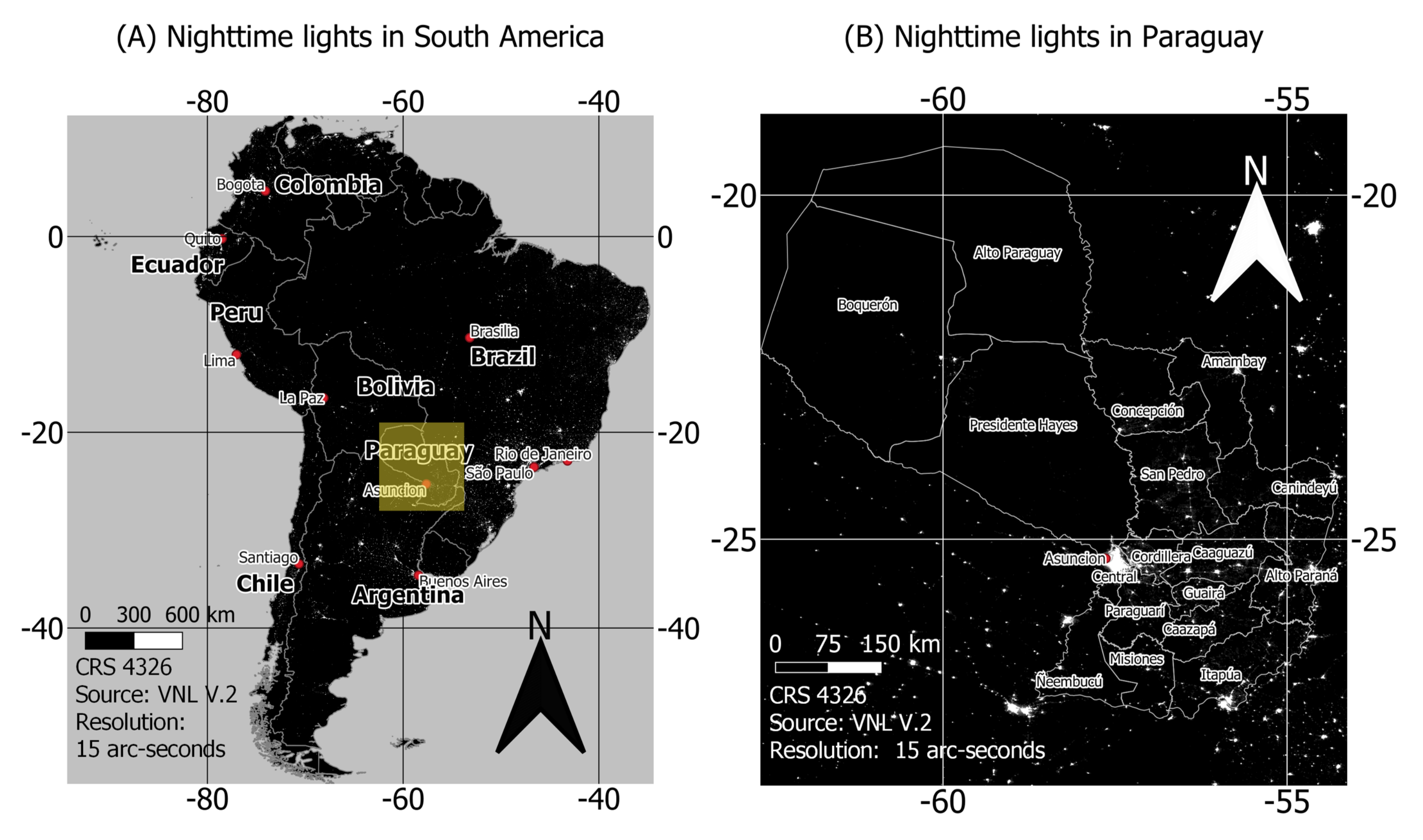
Our modeling approach estimates the parametric relationship between NTL and GDP at the subnational level in South American countries with official subnational GDP estimates, and employs out-of-sample prediction to estimate GDP in Paraguay’s departamentos. As we have annual VIIRS nightlights data, we build the GDP time series for each country between 2014 and 2019. We base our econometric specifications on the literature and assess their out-of-sample goodness-of-fit through cross-validation. For each country with data, we exclude the country, fit the model with the remaining countries, and calculate the difference between predicted and actual subnational GDP in the omitted country. Additionally, we assess the models by comparing the out-of-sample results for Paraguay with input–output estimations. To our knowledge, this is the first paper to study the NTL–GDP relationship exclusively in South America using VIIRS data. Recent work by Andreano et al. examines the relationship of NTL with poverty and inequality indicators in Latin America and the Caribbean [20]. However, the structural relationship of lights with poverty and inequality can be different from their relationship with GDP. The authors’ methods differ from ours as they use national parameters based on DMSP-OLS imagery to estimate subnational poverty levels while we use subnational parameters based on VIIRS imagery to estimate subnational GDP.

2.1. Study Area

The study area is the South American continent. Specifically, we include Argentina, Bolivia, Brazil, Chile, Colombia, Ecuador, and Peru in our analysis given the availability of subnational GDP data. Our focus is on the first subnational administrative unit (often referred to as admin-1). These units have different names in each country. For instance, they are called departamentos in Bolivia, Colombia, Paraguay, and Peru, provincias in Argentina and Ecuador, regiones in Chile, and estados in Brazil. We estimate models using a total of 127 subnational units from seven countries (note that in Argentina we only include the provincia of Buenos Aires due to GDP data availability). We then use parameter estimates from those models to predict GDP in the 18 Paraguayan departamentos. There is significant variation between admin-1 units in terms of geographical characteristics as they span the continent. Figure 1 shows examples of NTL images for South America and Paraguay; we provide details on the data in the following subsection.

2.2. Data

We obtain GDP data for the first-level administrative units in Bolivia [21], Brazil [22], Chile [23], Colombia [24], Ecuador [25], Peru [26], and Argentina [27] (only for Buenos Aires) from corresponding national offices. GDP data in these countries is usually estimated through the production (value-added) approach, and in some cases subnational GDP estimates are adjusted to sum to national GDP. In each case, we convert nominal GDP to constant 2017 international dollars. For the calculations, we retrieve the national GDP in constant and current local currency units from the World Bank (NY.GDP.MKTP.PP.KD and NY.GDP.MKTP.CN) and calculate the implicit deflator. Finally, we multiply the subnational GDP by the national deflator in the corresponding year.
We retrieve the luminosity data from the Earth Observation Group repository that includes processed images of annual global VIIRS nighttime lights (Annual VNL V.2) [28]. The composites are generated after filtering sunlit and moonlit clouds, as well as removing outliers [29]. Annual images are produced by averaging monthly composites. Each composite has a resolution of 15 arc seconds (roughly 500 m at the equator). We use this product following the research of Gibson and Boe-Gibson [11], who find that the masked average radiance data in VNL V.2 has higher predictive power for subnational GDP (in both cross section and time-series) than the prior version of the product (Annual VNL V.1) and DMSP data. We use images from 2014 to 2019 and masked them to the South American continent. In some specifications, we construct subnational region population estimates using gridded population data from WorldPop for the seven countries in the GDP sample and for Paraguay from 2014 to 2019 [30]. The WorldPop product has a resolution of 30 arc seconds (~1km at the equator), and provides the population per kilometer squared in each grid cell. WorldPop population estimates are calibrated to total official national population. Table 2 shows descriptive statistics for GDP and NTL by country.
For the boundaries of countries and administrative units, we use the Global Administrative Areas Database [31]. Using these polygons, we sum luminosity and population at the departamento level. We also calculate the area per country. We use RStudio version 1.4.1103 for all the calculations and QGIS version 3.10.14 for creating maps In RStudio, we use the ‘raster’, ‘sf’, and ‘exactextractr’ packages to manipulate and make calculations with spatial and raster files, and ‘lme4’ for econometric analyses with random effects.

2.3. Empirical Strategy

We employ multiple econometric models to estimate the association between year-on-year changes in nightlights and subnational GDP in Bolivia, Brazil, Chile, Colombia, Ecuador, Peru, and Buenos Aires (Argentina). The econometric specifications are drawn from existing literature studying the NTL-GDP relationship [8,11,15,32]. We then use cross-validation to evaluate goodness-of-fit in our study context for each of these models. In addition, we use each model to estimate Paraguayan departamento-level GDP and evaluate the estimates against another study that uses a different approach. Finally, we use our preferred model to construct a time series of GDP estimates for each Paraguayan departamento, and validate the approach by comparing analogous estimates of Bolivian regions against official measures of these regions’ GDP.
Our basic specification is the following:
l o g ( G D P r c t ) = α + β 1 l o g ( N T L r c t ) + δ t + γ r + ϵ r c t
where G D P r c t is the gross output (in constant dollar terms) in subnational region r of country c in year t, and N T L r c t is the sum of nighttime lights within the region in year t. As both GDP and NTL are in logarithms, the parameter β 1 captures the NTL elasticity of GDP (a unitless measure representing the percentage change in GDP associated with a percentage change in NTL). δ t are year fixed effects that flexibly detrend the data and capture any changes in the satellite sensor over time. We include random effects γ r at either country or subnational levels, as they allow for out-of-sample prediction without dealing with country-specific intercepts of fixed-effects models [32]. α is the model’s constant term and ϵ r c t is the error term. In addition, we include a model allowing for nonlinearity in the NTL-GDP relationship by adding a quadratic term for nightlights— l o g 2 ( N T L ) —as follows [10,33]:
l o g ( G D P r c t ) = α + β 1 l o g ( N T L r c t ) + β 2 l o g 2 ( N T L r c t ) + δ t + γ r + ϵ r c t
Coefficients β 1 and β 2 in Equation (2) capture the quadratic relationship between GDP and NTL, while all other equation parameters remain the same. Equations (1) and (2) are parsimonious specifications as they are solely based on NTL. These specifications are used in the recent literature on the NTL-GDP relationship [11,15], as well as some of the first national-level NTL-GDP elasticity estimates [8]. We test this parsimony against a model that incorporates more independent variables including country-level fixed factors (national area and number of regions), following the setup of Lessman and Seidel [32]. The third model is summarized in the equation:
l o g ( G D P r c t ) = α + β 1 l o g ( N T L r c t ) + λ l o g ( P o p r c t ) + η l o g ( C o u n t r y G D P c t ) + κ l o g ( A r e a C o u n t r y c ) + ϕ l o g ( N u m b e r R e g i o n s c ) + δ t + γ r + ϵ r c t
where P o p r c t is the population of the administrative unit since this variable is correlated to subnational economic output. C o u n t r y G D P c t is the national GDP, A r e a C o u n t r y c is the country’s area measured in square kilometers, and N u m b e r R e g i o n s c is the total number of first-level administrative regions in the country. As above, coefficient β 1 describes the GDP-NTL relationship, while λ , η , κ , and ϕ are coefficients for population, country GDP, country area, and number of region variables, respectively. As in Equations (1) and (2), we add year fixed effects δ t to detrend the data and random effects γ r at country or subnational region level. α is the constant term and ϵ r c t is the regression error term.

2.4. Out-of-Sample Prediction

We estimate the econometric models and make out-of-sample predictions for Paraguayan departamentos using the parametric results from the model that performs best in cross-validation. Finally, we estimate GDP by calculating the share of each departamento in the national predicted GDP, calculated as the sum of the subnational predicted GDP. Then, we adjust the departamento GDP estimates so that they total the official national GDP (from the World Bank Data), as follows:
G D P * r c t = C o u n t r y G D P c t G D P r c t ^ G D P c t ^
where G D P * r c t is the final GDP estimate for departamentor in year t, C o u n t r y G D P c t is the observed official national GDP, G D P r c t ^ is the predicted gross departmental product calculated using the model parameters, and G D P c t ^ is the national sum of the predicted departmental products. This approach differs from previous work [5,6,34] as we are distributing an official national GDP based on the econometric models instead of directly predicting GDP or growth from the model. Additionally, we consider a naïve approach where we distribute the official national GDP estimates based only on the distribution of NTL and compare these results against our models.

3. Results

Figure 2 plots the logarithm of subnational GDP for the seven countries against the logarithm of the sum of NTL. The correlation between both variables is 0.95, and the linear fit has a slope of 0.86. The relationship supports using linear models for these seven countries for out-of-sample prediction in Paraguayan departamentos. While the raw data support a linear fit, there is some variation across locations in how well the regression line fits the data. For instance, the Colombian departamento of Chocó and the Ecuadorian provincia of Sucumbios have the largest deviations from the linear fit. Both of these regions have lower population density than most other parts of their respective countries, with Sucumbios producing a lot of oil. As we further explain in the Discussion, the subnational NTL-GDP relationship has been shown to be different in low population density, high informality, and heavily agricultural areas.
Table 3 shows results based on the more parsimonious approach in Equation (1). Column 3.1 shows the association between subnational NTL and GDP, including year fixed effects to detrend the data and control for any changes in the satellite sensor over time. The NTL elasticity of GDP (parameter β 1 in Equation (1)) is 0.87 in this model, suggesting that a 1% increase in NTL is associated with a 0.87% increase in GDP. Column 3.2 shows the result after including a quadratic term for NTL (Equation (2)), indicating a statistically significant nonlinearity consistent NTL changing less with GDP changes at very high levels of GDP and NTL. Linear results vary only slightly when adding country-level random effects in column 3.3, resulting in a GDP-NTL elasticity of 0.90. In contrast, column 3.4 includes random effects at the first-level administrative unit, and the elasticity becomes 0.25. In column 3.5, we include both country-level and first-administrative-level random effects and obtain an elasticity of 0.24. These results are expected since the coefficient of interest is calculated based on variation within a subnational region over time, without using the cross-sectional association of NTL and GDP. R 2 in the specifications is high (notably, model 3.1 with only year fixed effects and no random effects has an R 2 of 0.90). For models 3.3, 3.4, and 3.5, we show the marginal R 2 (the variance explained by the model excluding random effects) as this is the explanatory power relevant for out-of-sample prediction in a different country. The low marginal R 2 in columns 3.4 and 3.5 implies that once we include random effects for first-level administrative units, variation in nightlights explains less of the GDP variation.
Table 4 shows results from the model in Equation (3), which includes more predictive variables following examples in the literature [32]. As all variables are in logarithms, each coefficient can be interpreted as an elasticity. Model 4.1 includes only nightlights and the region’s population in the specification, and indicates that a 1% higher sum of nightlights is associated with 0.48% higher regional GDP, while a 1% higher level of population is associated with a 0.55% higher level of regional GDP. Notice that the R 2 does not change notably from models in Table 3, which suggests that NTL have significant predictive power by themselves.
Model 4.2 adds the log of national GDP, which in that model is not statistically significant. Model 4.3 adds the log of country area and number of administrative regions. The coefficients on nightlights and region population remain very similar to 4.1 and 4.2, while the 0.20 coefficient on country GDP suggests that controlling for other variables, a 1% higher national GDP is associated with a 0.2% higher regional GDP (holding nightlights constant). Country area and the number of regions in the country are both negatively associated to regional GDP, and coefficients suggest that countries with 1% more area have 0.17% lower regional GDP and those with 1% greater number of regions have 0.15% lower regional GDP. In columns 4.4 and 4.5, we add country-level and admin-1 level random effects, respectively. Country-level random effects in 4.4 absorb the explanatory power of the country-level variables, while nightlights and population remain statistically significant and their magnitudes are similar to those in previous columns. Adding admin-1 random effects reduces the GDP-NTL elasticity to 0.21, and increases the population coefficient to 0.79. The country-level coefficients for GDP, area and number of regions are all significant and of larger magnitude than in column 4.3. We find similar results when adding both country-level and admin-1 level random effects in column 4.6.
In summary, Table 4 indicates that the GDP-NTL elasticity ranges between 0.48 and 0.53 when including the population, national GDP, national area, and number of subnational regions, and it is reduced to 0.21–0.24 when including admin-1 level random effects. R 2 remains high at 0.92–0.93 even after excluding the explanatory power of the random effects (columns 4.4–4.6).
As we are interested in out-of-sample prediction, we cross-validate the fit of the different models against each country with available subnational GDP data. That is, we fit the models excluding one country and then use the parametric results to predict GDP in the subnational units of the excluded country as described in Section 2.4. Then, we calculate the root mean square error of the predicted GDP versus the observed as a percentage of the mean subnational GDP in that country. We set the random effect value to zero in the predictions where this approach was used. Table 5 displays the deviations for each model and country. The column label is the number of the table and column, i.e., column 3.2 is the second model in Table 3. Additionally, column “base” represents the approach where we distribute the observed national GDP only based on each subnational region’s share of the national sum of NTL. Results are mixed. For Bolivia, Chile, Colombia, Ecuador, and Peru, models 4.1–4.6 appear to perform better, while for Brazil the best model is 3.2. Model 3.5 has the lowest predictive power for all countries. In all cases, the base model does not perform better than the parametric approaches. The goodness-of-fit of each model also varies across countries. Bolivia has the smallest mean deviation relative to the mean regional GDP with a 19 percent difference. Meanwhile, we see considerably higher deviation in the case of Colombia or Peru. This result is consistent with some variation in the GDP–NTL relationship, which could be due either to differences across countries in measurement error of subnational GDP, or to differences in the structural GDP-NTL relationship. The final row shows the average RMSE across countries for each model. By this metric, we take model 4.4 as our preferred model for prediction in a country out-of-sample (Paraguay).
A second approach to test model fit is to make predictions for Paraguay and compare them against an estimate of Paraguayan subnational GDP using input–output accounting [35]. These estimates use the Interregional Input–Output Adjustment System (IIOAS) and a general equilibrium model to calculate the 2014 GDP in the 17 departamentos and the capital Asunción. They use multiple national datasets to characterize 33 economic sectors including household surveys, the 2011 economic census, population projections, and the 2008 agricultural census. To compare, we predict 2014 GDP in Paraguayan departamentos based on our parametric models.
Table 6 shows the national GDP share of every departamento according to each model, with the last column showing the estimates based on the IIOAS. The first thing to notice is that size of divergence between our results and the IIOAS estimates varies across departamentos. The highest root-mean-square deviation relative to IIOAS are from models 3.4 and 3.5, while other models have a deviation between 2.4 and 3.0 percentage points. The best fit is the naïve model in which we distribute GDP according to each department’s share of the national sum of NTL (column “base”). Models 4.1 and 4.4 resulted in the next best fit, but their deviations are only slightly lower than those in models 4.2 and 4.3.
Given our two goodness-of-fit exercises, we move forward with model 4.4 and the “base” model for prediction of department-level GDP in Paraguay. The temporal frequency of NTL imagery allows for estimating and analyzing departamento-level economic trends. Figure 3 shows these series for the departamentos of Alto Paraná, Asunción, Caaguazú, Central, and Itapúa, and the sum of the rest of the departamentos. The red line is the GDP prediction based on model 4.4 in Table 4, and the dotted line is based on the naïve (“base”) model. All departamentos except Asunción show an increase of GDP over time. Both models are based on NTL change, yet while they exhibit similar trends, predicted levels vary significantly across the models. On average, model 4.4 is 8.6% lower in Alto Paraná relative to the naïve model, 8.9% in Asunción, and 5.5% in Itapúa. Meanwhile, it is 12.6% higher in Caaguazú and 9.9% in Central. In the sum of other departments, model 4.4 is 2.6% lower than the base model on average. To our knowledge, this is the first time series of GDP for Paraguayan departamentos.
In order to gauge the accuracy of our subnational GDP time series, we compare the predictions against data on subnational GDP over time in Bolivia (the country with the best fit in Table 5). Figure 4 shows the time series for subnational GDP for all nine provinces of Bolivia, with the blue line indicating the official data on provincial GDP. Overall, model 4.4 tracks the official measure of GDP better than the naïve model, consistent with Table 5 showing that 4.4 is the better fit for Bolivia.
Figure 5 maps the average GDP per departamento in Paraguay. The Chaco region in the northwest part of the country covers a significant portion of national land area, however economic output there is the lowest. Our estimates clearly show two economic poles: one in the area of Central and Asunción and the other in the east around Alto Paraná. These are also the areas where most of the population lives.

4. Discussion

In this analysis, we employ nightlights imagery from the VIIRS VNL V.2 product to study the predictive relationship between lights and GDP at subnational level and present a method to make out-of-sample predictions for first-level administrative units. We parameterize the predictive relationship using econometric specifications from the NTL-GDP literature and estimate the parameters for subnational units in Paraguay’s neighboring countries. The first set of regressions in Table 3 shows a NTL-GDP elasticity ( β 1 ) from 0.87 in pooled regression (Column 3.1) to 0.24 when incorporating country and first-administrative level random effects (Column 3.5). While we show evidence for nonlinearity in the relationship (Table 3, Column 3.2), a quadratic model performs less well in out-of-sample prediction. In a second set of econometric specifications (Table 4), we add additional country-level variables to increase the predictive power of our estimates. After controlling for these, the NTL-GDP elasticity hovers at 0.46–0.48, and reduces to 0.21–0.24 when including admin-1 level random effects.
Additionally, we use cross-validation to assess the predictive skill of each econometric specification by leaving one country out, estimating the model on remaining countries, and evaluating the predictive fit in the omitted country against official subnational GDP data. The root mean square error varies across countries. In our preferred econometric specification (Table 4, Column 4.4), the root mean square errors range from 19.9% of mean regional GDP in Bolivia to 64.8% in Colombia. We also compare out-of-sample predictions for Paraguay against prior estimates based on input–output methods. On average, the predictions deviate by 2.7 percentage points of national GDP in our preferred econometric model and 2.4 points with the naïve model based only on lights distribution. When comparing time-series predictions against Bolivian subnational data, we note that the predictions are generally similar to official estimates though deviations persist in some regions. Such results suggest that researchers should be cautious when using NTL to estimate GDP since predictive power can vary across subnational units. Nevertheless, this approach can be helpful for countries that lack subnational economic statistics.
Subnational GDP predictions highlight the variation in the economic size across Paraguayan departamentos. Using the results from model 4.4, the largest department in terms of economic size is Central, whose average 2014–2019 GDP was 25.8 billion dollars (PPP, international 2017 dollars) or ~30.8% of the national economy. This is very similar to the share of the Paraguayan population living there in 2019. The second largest departamento was Alto Paraná with $11.2 billion on average during the same period or around 13.4% of the national GDP. The third largest departamento was Itapúa with $7.6 billion, while Asunción was the fourth subnational economy. In contrast, the smallest economy was Alto Paraguay with an average of $0.16 billion.
Each department-level GDP trend in Figure 3 results from two features in our modeling methodology: the trend in the overall economy of the country and the trend in the department’s share in the model prediction (model 4.4) or sum of NTL (the “base” model). The trends of the five largest departmental economies suggest economic growth over the period, except in Asunción. The graphs also suggest that country’s economic slowdown in 2019 (during which there was a 0.4% decline in national GDP [36]) may have had different impacts across departments.
Our cross-validation and comparison to the IIOAS estimates suggest that VIIRS-based prediction can provide helpful estimates of subnational GDP in countries that do not measure or report it. While our preferred model produces subnational GDP series that matches Bolivian data well (and Table 5 shows model 4.4 has an overall RMSE in Bolivia of 19.9% of mean subnational GDP), it is worth noting that the prediction error in other countries can become quite significant (model 4.4 has an average RMSE across countries of 41% of subnational GDP, and as high as 65% in Colombia).

Limitations and Future Work

Other considerations about our approach are warranted. First, agriculture, fishing, and forestry represent ~10% of the Paraguayan economy, and these activities concentrate more in some regions. Other work has found that NTL-based GDP estimates for the U.S. perform less well in subnational regions with larger agricultural share [15], and that the agricultural share in GDP is higher in African countries where GDP was underestimated by NTL (although the difference in the agriculture share across underestimated and overestimated GDP is only 3.6 percentage points, 29.7 versus 26.1 percent) [5]. Nevertheless, our GDP predictions are likely less accurate in departamentos where agriculture plays a large role in the economy.
Second, variation in levels of informality within countries may affect the stability of the GDP-NTL fit across countries and subnational regions. The activities in the informal sector are likely undetected in GDP measurements, and yet are captured by NTL data. If countries in the sample have lower informality levels, we may predict higher GDP than in official data for other regions with high informality, which would reduce goodness-of-fit even though the NTL-based GDP estimates may be better capturing economic activity than official estimates.
More generally, another potential challenge for our out-of-sample prediction approach is the stability of parameters [10]. If the structural GDP–NTL relationship varies across countries or subnational regions, out-of-sample prediction requires understanding which factors drive that instability and adjusting the prediction using those factors. For example, if the GDP–NTL elasticity is structurally different in agricultural or low population density areas [12,17], this may suggest that our approach is not as precise in areas such as Alto Paraguay and Boquerón, where population density is low. In the comparison in Table 6, we can see that our estimates are lower than the IIOAS-based estimates for these two departamentos. A second source of potential parameter instability results from the nature of economic growth at different stages of development. Countries and regions experiencing economic growth at early stages of development often exhibit expansion of infrastructure, whereas more advanced economies grow with productivity increases in industry and services [33]. Our sample of countries do not seem to exhibit such nonlinearity in the GDP-NTL relationship, as shown in Figure 2, though it is possible that Paraguay might have a nonlinear relationship at the departamento level.
Finally, these methods are unlikely to provide accurate prediction of seasonal or year-on-year GDP changes for Paraguayan departamentos. Our own results show that using random effects at the subnational level reduces the marginal R 2 considerably (in model 3.5 of Table 3 the marginal R 2 is just 0.10). This suggests that after controlling for cross-sectional variation, the predictive power of lights on changes in GDP is rather low. This is consistent with other work [19], in which authors argue that errors in the NTL satellite images, the effect of seasons, or more likely the smaller variation of GDP growth relative to cross-sectional changes might be to blame for lower predictive power of NTL on annual changes in GDP within a location. In general terms, the predictive power of NTL may be more appropriate for cross-sectional estimates. In our setting, this suggests that relying on NTL to estimate unmeasured subnational GDP levels is appropriate, but using lights to measure year-on-year subnational GDP growth rates is likely less accurate and limits the ability of NTL to provide insights into the short-term economic dynamics in Paraguayan departamentos. Nevertheless, NTL can usefully predict GDP at the first-administrative level, especially in those cases where subnational economic data are lacking.

5. Conclusions

Designing good economic policy at subnational scale, including localizing the Sustainable Development Goals, requires accurate economic statistics at appropriate geographic resolution. However, the lack of resources in many national statistical offices hinders systematic collection and publication of such subnational economic data. While not a substitute for investing in national accounts and economic censuses, remote sensing can generate subnational estimates at multiple scales. We build on existing literature exploring the relationship between NTL imagery and GDP to develop a method to estimate GDP at the first administrative level for Paraguay, specifically by fitting models on data from countries in South America that have official GDP statistics at this level. Additionally, we use two validation approaches in the process of model selection. Remotely sensed imagery has an important role to play in constructing economic and other indicators to monitor progress towards the Sustainable Development Goals. This is particularly the case in countries without resources for robust ground-level data collection that is representative at subnational scales.

Author Contributions

G.C.M. and M.R.-H. contributed equally to this work. All authors have read and agreed to the published version of the manuscript.

Funding

This research received no external funding.

Institutional Review Board Statement

Not applicable.

Informed Consent Statement

Not applicable.

Data Availability Statement

Data will be made available online upon publication.

Conflicts of Interest

The authors declare no conflict of interest.

References

  1. Lenzen, M.; Geschke, A.W.J. Implementing the material footprint to measure progress towards Sustainable Development Goals 8 and 12. Nat. Sustain. 2021. [Google Scholar] [CrossRef]
  2. Peña-Sánchez, A.R.; Ruiz-Chico, J.; Jiménez-García, M.; López-Sánchez, J.A. Tourism and the SDGs: An Analysis of Economic Growth, Decent Employment, and Gender Equality in the European Union (2009–2018). Sustainability 2020, 12, 5480. [Google Scholar] [CrossRef]
  3. Liu, S. Interactions between industrial development and environmental protection dimensions of Sustainable Development Goals (SDGs): Evidence from 40 countries with different income levels. Environ.-Socio-Econ. Stud. 2020, 8, 60–66. [Google Scholar] [CrossRef]
  4. Kynčlová, P.; Upadhyaya, S.; Nice, T. Composite index as a measure on achieving Sustainable Development Goal 9 (SDG-9) industry-related targets: The SDG-9 index. Appl. Energy 2020, 265, 114755. [Google Scholar] [CrossRef]
  5. Bundervoet, T.; Maiyo, L.; Sanghi, A. Bright Lights, Big Cities: Measuring National and Subnational Economic Growth in Africa from Outer Space, with an Application to Kenya and Rwanda; World Bank Policy Research Working Paper; World Bank: Washington, DC, USA, 2015. [Google Scholar]
  6. Rangel-Gonzalez, E.; Llamosas-Rosas, I. An Alternative Method to Measure Non-Registered Economic Activity in Mexico Using Satellite Nightlights. 2019. Available online: https://urldefense.proofpoint.com/v2/url?u=https-3A__www.imf.org_-2D_media_Files_Conferences_2019_7th-2Dstatistics-2Dforum_session-2Diii-2Dgonzalez.ashx&d=DwIGAw&c=-35OiAkTchMrZOngvJPOeA&r=HZF_zs-aVMZKPZ_P0n0ubz4cB0YKCDtdn1Wbk6NWga0&m=PWwAzqm6DIUKgu9mMAbAUxBcJE_dDR6L3__EsqzSAb4GyLqJ032YT7yMXytIjExc&s=L6CmyrqjtDPX9jtxzWFOfU0aalhAZwGNtbx-WWGZW0g&e= (accessed on 1 July 2021).
  7. Chen, X.; Nordhaus, W.D. Using luminosity data as a proxy for economic statistics. Proc. Natl. Acad. Sci. USA 2011, 108, 8589–8594. [Google Scholar] [CrossRef] [Green Version]
  8. Henderson, J.V.; Storeygard, A.; Weil, D.N. Measuring economic growth from outer space. Am. Econ. Rev. 2012, 102, 994–1028. [Google Scholar] [CrossRef] [Green Version]
  9. Hodler, R.; Raschky, P.A. Regional Favoritism. Q. J. Econ. 2014, 129, 995–1033. [Google Scholar] [CrossRef]
  10. Bickenbach, F.; Bode, E.; Nunnenkamp, P.; Söder, M. Night lights and regional GDP. Rev. World Econ. 2016, 152, 425–447. [Google Scholar] [CrossRef] [Green Version]
  11. Gibson, J.; Boe-Gibson, G. Nighttime Lights and County-Level Economic Activity in the United States: 2001 to 2019. Remote Sens. 2021, 13, 2741. [Google Scholar] [CrossRef]
  12. Chen, X.; Nordhaus, W. A test of the new VIIRS lights data set: Population and economic output in Africa. Remote Sens. 2015, 7, 4937–4947. [Google Scholar] [CrossRef] [Green Version]
  13. Gibson, J.; Olivia, S.; Boe-Gibson, G. Night lights in economics: Sources and uses. J. Econ. Surv. 2020, 34, 955–980. [Google Scholar] [CrossRef]
  14. Elvidge, C.D.; Baugh, K.E.; Zhizhin, M.; Hsu, F.C. Why VIIRS data are superior to DMSP for mapping nighttime lights. Proc.-Asia-Pac. Adv. Netw. 2013, 35, 62. [Google Scholar] [CrossRef] [Green Version]
  15. Gibson, J.; Olivia, S.; Boe-Gibson, G.; Li, C. Which night lights data should we use in economics, and where? J. Dev. Econ. 2021, 149, 102602. [Google Scholar] [CrossRef]
  16. Shi, K.; Yu, B.; Huang, Y.; Hu, Y.; Yin, B.; Chen, Z.; Chen, L.; Wu, J. Evaluating the ability of NPP-VIIRS nighttime light data to estimate the gross domestic product and the electric power consumption of China at multiple scales: A comparison with DMSP-OLS data. Remote Sens. 2014, 6, 1705–1724. [Google Scholar] [CrossRef] [Green Version]
  17. Gibson, J. Better night lights data, for longer. Oxf. Bull. Econ. Stat. 2021, 83, 770–791. [Google Scholar] [CrossRef]
  18. Dai, Z.; Hu, Y.; Zhao, G. The suitability of different nighttime light data for GDP estimation at different spatial scales and regional levels. Sustainability 2017, 9, 305. [Google Scholar] [CrossRef] [Green Version]
  19. Chen, X.; Nordhaus, W.D. VIIRS nighttime lights in the estimation of cross-sectional and time-series GDP. Remote Sens. 2019, 11, 1057. [Google Scholar] [CrossRef] [Green Version]
  20. Andreano, M.S.; Benedetti, R.; Piersimoni, F.; Savio, G. Mapping Poverty of Latin American and Caribbean Countries from Heaven Through Night-Light Satellite Images. Soc. Indic. Res. Int. Interdiscip. J.-Qual.-Life Meas. 2021, 156, 533–562. [Google Scholar] [CrossRef]
  21. Instituto Nacional de Estadística (Bolivia). Producto Interno Bruto Departamental. Available online: https://urldefense.proofpoint.com/v2/url?u=https-3A__www.ine.gob.bo_index.php_estadisticas-2Deconomicas_pib-2Dy-2Dcuentas-2Dnacionales_producto-2Dinterno-2Dbruto-2Ddepartamental_producto-2Dinterno-2Dbruto-2Ddepartamental_-231589484093225-2Db57379da-2Db2f6&d=DwIGAw&c=-35OiAkTchMrZOngvJPOeA&r=PIf8F-g-Zjd8VnENokL6gg&m=bzB_ZWonfTu_eRX7j8_K06pySrZt4zSW46DERrsUXrgo6UIANlbF1ziJhBHHW6jf&s=E4H3pBTBVA1l8W9NNr2Vx6et25n3KeIfyPh82yzXuMk&e= (accessed on 1 March 2021).
  22. Instituto Brasileiro de Geografia e Estatística. Produto Interno Bruto dos Municípios. Available online: https://urldefense.proofpoint.com/v2/url?u=https-3A__www.ibge.gov.br_estatisticas_economicas_contas-2Dnacionais_9088-2Dproduto-2Dinterno-2Dbruto-2Ddos-2Dmunicipios.html-3F-3D-26t-3Dresultados&d=DwIGAw&c=-35OiAkTchMrZOngvJPOeA&r=PIf8F-g-Zjd8VnENokL6gg&m=bzB_ZWonfTu_eRX7j8_K06pySrZt4zSW46DERrsUXrgo6UIANlbF1ziJhBHHW6jf&s=zEc8uS6Rj2qt6bprOC3BSYWaUSJs7-SlTLGeSmKEAnY&e= (accessed on 1 March 2021).
  23. Banco Central de Chile. Producto Interno Bruto Regional. Available online: https://urldefense.proofpoint.com/v2/url?u=https-3A__si3.bcentral.cl_estadisticas_Principal1_Excel_CCNN_regional_excel.html&d=DwIGAw&c=-35OiAkTchMrZOngvJPOeA&r=PIf8F-g-Zjd8VnENokL6gg&m=bzB_ZWonfTu_eRX7j8_K06pySrZt4zSW46DERrsUXrgo6UIANlbF1ziJhBHHW6jf&s=MayuP-aGdpug4SaemNx5TxnUPyDqqOjn_OKo2YxT6M8&e= (accessed on 1 March 2021).
  24. Dirección Nacional de Estadística (Colombia). PIB por Departamento. Available online: https://urldefense.proofpoint.com/v2/url?u=https-3A__www.dane.gov.co_index.php_estadisticas-2Dpor-2Dtema_cuentas-2Dnacionales_cuentas-2Dnacionales-2Ddepartamentales&d=DwIGAw&c=-35OiAkTchMrZOngvJPOeA&r=PIf8F-g-Zjd8VnENokL6gg&m=bzB_ZWonfTu_eRX7j8_K06pySrZt4zSW46DERrsUXrgo6UIANlbF1ziJhBHHW6jf&s=EbP0tikaQ_5u6kTRPpgCuYtvPFTyCbGTo5Ja-773E1s&e= (accessed on 1 March 2021).
  25. Banco Central del Ecuador. Cuentas Nacionales Regionales. Available online: https://urldefense.proofpoint.com/v2/url?u=https-3A__contenido.bce.fin.ec_documentos_Estadisticas_SectorReal_CuentasProvinciales_Indice.htm&d=DwIGAw&c=-35OiAkTchMrZOngvJPOeA&r=PIf8F-g-Zjd8VnENokL6gg&m=bzB_ZWonfTu_eRX7j8_K06pySrZt4zSW46DERrsUXrgo6UIANlbF1ziJhBHHW6jf&s=iLNaJkSnq6BVMfOdIB58ZP4V-tbZfIImZv5Q0y5tIko&e= (accessed on 1 March 2021).
  26. Instituto Nacional de Estadística e Informática (Perú). Producto Bruto Interno por Departamentos (Cifras Preliminares). Available online: https://urldefense.proofpoint.com/v2/url?u=https-3A__www.inei.gob.pe_estadisticas_indice-2Dtematico_producto-2Dbruto-2Dinterno-2Dpor-2Ddepartamentos-2D9089_&d=DwIGAw&c=-35OiAkTchMrZOngvJPOeA&r=PIf8F-g-Zjd8VnENokL6gg&m=bzB_ZWonfTu_eRX7j8_K06pySrZt4zSW46DERrsUXrgo6UIANlbF1ziJhBHHW6jf&s=nYm7-FChipHZVrZrbR_iR6ZDcK_NI7qZZnsNceiK4hE&e= (accessed on 1 March 2021).
  27. Dirección Provincial de Estadística (Buenos Aires, Argentina). Producto Bruto Geografico—Provincia de Buenos Airea-Año 2018 y Serie 2004–2018. Base 2004. Available online: https://urldefense.proofpoint.com/v2/url?u=http-3A__www.estadistica.ec.gba.gov.ar_dpe_index.php_prensa2018_513-2Dpbg-2D2018&d=DwIGAw&c=-35OiAkTchMrZOngvJPOeA&r=PIf8F-g-Zjd8VnENokL6gg&m=bzB_ZWonfTu_eRX7j8_K06pySrZt4zSW46DERrsUXrgo6UIANlbF1ziJhBHHW6jf&s=SS6uLjNrvM00S_AbXbVPr5kVfW5vNgPUwlevn5Stto0&e= (accessed on 1 March 2021).
  28. Earth Observation Group. Annual VNL V2. Available online: https://urldefense.proofpoint.com/v2/url?u=https-3A__eogdata.mines.edu_products_vnl_&d=DwIGAw&c=-35OiAkTchMrZOngvJPOeA&r=PIf8F-g-Zjd8VnENokL6gg&m=bzB_ZWonfTu_eRX7j8_K06pySrZt4zSW46DERrsUXrgo6UIANlbF1ziJhBHHW6jf&s=4h_UB5Vr0nCzl-srRahNzjnTo1V2i3fp-eY9C1M_21k&e= (accessed on 25 June 2021).
  29. Elvidge, C.D.; Zhizhin, M.; Ghosh, T.; Hsu, F.C.; Taneja, J. Annual time series of global VIIRS nighttime lights derived from monthly averages: 2012 to 2019. Remote Sens. 2021, 13, 922. [Google Scholar] [CrossRef]
  30. WorldPop—School of Geography and Environmental Science, University of Southampton; Department of Geography and Geosciences, University of Louisville; Departement de Geographie, Universite de Namur) and Center for International Earth Science Information Network (CIESIN), Columbia University. Global High Resolution Population Denominators Project—Funded by The Bill and Melinda Gates Foundation (OPP1134076). 2018. Available online: https://urldefense.proofpoint.com/v2/url?u=http-3A__www.worldpop.org&d=DwIGAw&c=-35OiAkTchMrZOngvJPOeA&r=PIf8F-g-Zjd8VnENokL6gg&m=bzB_ZWonfTu_eRX7j8_K06pySrZt4zSW46DERrsUXrgo6UIANlbF1ziJhBHHW6jf&s=Npvvoxj00rmBkqe5wcp327U4641JFV1rLztPhojtpLQ&e= (accessed on 25 June 2021).
  31. Database of Global Administrative Boundaries (GADM) Version 3.6. 2018. Available online: https://urldefense.proofpoint.com/v2/url?u=http-3A__www.gadm.org&d=DwIGAw&c=-35OiAkTchMrZOngvJPOeA&r=PIf8F-g-Zjd8VnENokL6gg&m=bzB_ZWonfTu_eRX7j8_K06pySrZt4zSW46DERrsUXrgo6UIANlbF1ziJhBHHW6jf&s=CLYS64gqYBnjI2ZUN3VbprAA3HVfocnyt_Xn9SqAWbU&e= (accessed on 25 June 2021).
  32. Lessmann, C.; Seidel, A. Regional inequality, convergence, and its determinants—A view from outer space. Eur. Econ. Rev. 2017, 92, 110–132. [Google Scholar] [CrossRef] [Green Version]
  33. Hu, Y.; Yao, J. Illuminating economic growth. J. Econ. 2021. [Google Scholar] [CrossRef]
  34. Martinez, L.R. How Much Should We Trust the Dictator’s GDP Growth Estimates; Becker Friedman Institute for Economics Working Paper 2021-78; University of Chicago: Chicago, IL, USA, 2021. [Google Scholar]
  35. Haddad, E.; Perobelli, F.; Castro, G.; Araújo, I.; Ramirez-Alvarez, P.E.; Fernandes, R. Tool Kits in Multi-Regional and Multi-Sectoral General Equilibrium Modeling for Paraguay; Technical Report; Núcleo de Economia Regional e Urbana da Universidade de São Paulo (NEREUS): São Paulo, Brazil, 2021. [Google Scholar]
  36. World Bank. GDP Growth (Annual %)—Paraguay. Available online: https://urldefense.proofpoint.com/v2/url?u=https-3A__data.worldbank.org_indicator_NY.GDP.MKTP.KD.ZG-3Flocations-3DPY_&d=DwIGAw&c=-35OiAkTchMrZOngvJPOeA&r=PIf8F-g-Zjd8VnENokL6gg&m=bzB_ZWonfTu_eRX7j8_K06pySrZt4zSW46DERrsUXrgo6UIANlbF1ziJhBHHW6jf&s=Uz62gYOqjg4_NBxJIM2baYfQmuHDHBW6KxVwu0h6uHQ&e= (accessed on 12 December 2021).
Figure 1. Example of 2019 VIIRS (VNL2) images clipped to (A) South America and (B) Paraguay polygons.
Remotesensing 14 01150 g001
Figure 2. Scatterplot of subnational ln(GDP) and ln(NTL).
Remotesensing 14 01150 g002
Figure 3. Time series of subnational GDP from model in Table 4, Column 4.4 and the naïve model (“base”).
Remotesensing 14 01150 g003
Figure 4. Time series of Bolivia’s subnational GDP from model 4.4 in Table 4, the naïve model (“base”), and the official measure of GDP.
Remotesensing 14 01150 g004
Figure 5. Estimated distribution of Paraguayan GDP in constant 2017 billion dollars and sum of NTL by department (2014–2019 averages). Estimates are based on model 4.4.
Remotesensing 14 01150 g005
Table 1. Indicators from the global indicator framework for the Sustainable Development Goals and targets that require GDP estimates.
#Indicator
1.5.2Direct economic loss attributed to disasters in relation to global gross domestic product (GDP)
7.3.1Energy intensity measured in terms of primary energy and GDP
8.1.1Annual growth rate of real GDP per capita
8.2.1Annual growth rate of real GDP per employed person
8.4.1/12.2.1Material footprint, material footprint per capita, and material footprint per GDP
8.4.2Domestic material consumption, domestic material consumption per capita, and domestic material consumption per GDP
8.9.1Tourism direct GDP as a proportion of total GDP and in growth rate
9.2.1Manufacturing value added as a proportion of GDP and per capita
9.4.1CO2 emission per unit of value added
9.5.1Research and development expenditure as a proportion of GDP
10.4.1Labor share of GDP
11.5.2Direct economic loss in relation to global GDP, damage to critical infrastructure and number of disruptions to basic services, attributed to disasters
12.2.2Domestic material consumption, domestic material consumption per capita, and domestic material consumption per GDP
12.c.1Amount of fossil fuel subsidies (production and consumption) per unit of GDP
14.7.1Sustainable fisheries as a proportion of GDP in small island developing States, least developed countries and all countries
17.1.1Total government revenue as a proportion of GDP, by source
17.3.2Volume of remittances (in United States dollars) as a proportion of total GDP
17.13.1Macroeconomic Dashboard
Table 2. Descriptive Statistics at Admin-1 Subnational Level.
ARGBOLBRACHLCOLECUPRYPER
Av. GDP353.8510.24113.6627.2621.577.56NA13.76
[5.03][9.27][190.09][44.69][40.87][12.82]NA[27.46]
Av. log(NTL)11.549.9512.1110.349.279.329.419.52
[0.86][1.27][1.06][1.04][1.84][1.31][1.08][0.94]
Regions1 *9271632241826
Note: * Argentina has 24 regions, but we include data for Buenos Aires province only. Standard deviations are shown in brackets. GDP data in billion PPP (constant 2017 international dollars).
Table 3. Predictive models for subnational GDP using nightlights.
(3.1)(3.2)(3.3)(3.4)(3.5)
log(NTL) 0.87 *** 0.28 *** 0.90 *** 0.25 *** 0.24 ***
( 0.01 ) ( 0.08 ) ( 0.01 ) ( 0.03 ) ( 0.03 )
log 2 (NTL) 0.03 ***
( 0.00 )
R 2 0.90 0.91 0.91 0.12 0.10
Observations761761761761761
Country Random EffectsNNYNY
Admin-1 Random EffectsNNNYY
Note: Standard errors in parentheses. Significance levels denoted at *** p < 0.001. All models include year fixed effects. For mixed models (3.3), (3.4), and (3.5), we show marginal R 2 that captures the variance explained by the model excluding the random effects.
Table 4. Predictive models for subnational GDP using nightlights.
(4.1)(4.2)(4.3)(4.4)(4.5)(4.6)
log(NTL) 0.48 *** 0.48 *** 0.46 *** 0.53 *** 0.21 *** 0.24 ***
( 0.02 ) ( 0.02 ) ( 0.02 ) ( 0.02 ) ( 0.03 ) ( 0.03 )
log(Pop) 0.55 *** 0.54 *** 0.58 *** 0.53 *** 0.79 *** 0.79 ***
( 0.02 ) ( 0.02 ) ( 0.03 ) ( 0.02 ) ( 0.04 ) ( 0.04 )
log(CountryGDP) 0.03 0.20 *** 0.45 0.62 *** 0.81 ***
( 0.02 ) ( 0.04 ) ( 0.25 ) ( 0.08 ) ( 0.12 )
log(CountryArea) 0.17 *** 0.39 0.43 *** 0.58 ***
( 0.03 ) ( 0.21 ) ( 0.07 ) ( 0.13 )
log(NumberRegions) 0.15 * 0.48 0.87 *** 1.09 ***
( 0.07 ) ( 0.45 ) ( 0.15 ) ( 0.31 )
R 2 0.95 0.95 0.95 0.93 0.92 0.92
Observations761761761761761761
Country Random EffectsNNNYNY
Admin-1 Random EffectsNNNNYY
Note: Standard errors in parentheses. Significance levels denoted at *** p < 0.001; * p < 0.05. All models include year fixed effects. For mixed models (4.4), (4.5), and (4.6), we show marginal R 2 that captures the variance explained by the model excluding the random effects.
Table 5. Root mean square error by country and model as percentage of national mean of subnational GDP (%).
Country(3.1)(3.2)(3.3)(3.4)(3.5)(4.1)(4.2)(4.3)(4.4)(4.5)(4.6)Base
Bolivia25.023.924.567.668.819.519.619.319.918.818.624.5
Brazil72.324.771.1149.8148.948.952.253.251.659.458.451.4
Chile60.243.254.9140.8142.028.028.127.126.830.430.137.8
Colombia96.892.594.4136.0151.969.070.367.564.866.762.385.9
Ecuador84.680.878.8138.4140.943.042.337.236.542.442.072.3
Peru95.381.090.6183.3183.952.355.146.046.951.949.870.8
Average72.457.769.1136.0139.443.544.641.741.144.943.557.1
Table 6. Department share of national 2014 GDP (%).
Departamento(3.1)(3.2)(3.3)(3.4)(3.5)(4.1)(4.2)(4.3)(4.4)(4.5)(4.6)BaseIIOAS
Alto Pry.0.30.40.32.62.70.20.20.20.20.20.20.20.5
Alto Paraná14.013.914.27.97.813.313.213.213.512.312.515.016.5
Amambay3.23.23.15.25.22.52.52.42.42.42.42.81.8
Asunción10.19.910.27.27.29.09.19.09.18.48.510.418.6
Boquerón1.41.51.34.04.10.90.90.90.90.90.91.12.2
Caaguazú6.36.16.36.36.37.07.07.06.97.57.56.05.1
Caazapá2.02.11.94.54.62.02.02.01.92.42.31.61.4
Canindeyú3.23.13.15.15.22.92.92.92.83.13.02.73.0
Central24.225.325.29.39.130.029.630.330.629.430.228.431.3
Concepción3.43.33.35.25.33.13.23.13.03.33.22.91.6
Cordillera4.54.44.45.75.74.14.14.14.04.24.14.11.7
Guairá3.03.02.95.15.12.82.82.82.73.02.92.51.7
Itapúa9.69.49.67.17.09.19.19.19.28.88.99.77.0
Misiones2.72.62.64.94.91.91.91.91.81.81.82.20.9
Ñeembucú1.71.81.64.34.41.21.31.21.21.31.21.41.0
Paraguarí3.02.92.95.05.13.03.13.02.93.43.32.51.5
Pte. Hayes1.91.91.84.44.51.51.61.51.51.71.61.51.8
San Pedro5.45.25.36.06.05.55.55.55.45.85.75.02.4
Deviation *3.02.92.96.76.82.72.82.82.73.02.92.4
* Root-mean-square deviation from IIOAS measured in national GDP percentage points.
Publisher’s Note: MDPI stays neutral with regard to jurisdictional claims in published maps and institutional affiliations.

