Banana Fusarium Wilt Disease Detection by Supervised and Unsupervised Methods from UAV-Based Multispectral Imagery

Abstract

Banana Fusarium wilt (BFW) is a devastating disease with no effective cure methods. Timely and effective detection of the disease and evaluation of its spreading trend will help farmers in making right decisions on plantation management. The main purpose of this study was to find the spectral features of the BFW-infected canopy and build the optimal BFW classification models for different stages of infection. A RedEdge-MX camera mounted on an unmanned aerial vehicle (UAV) was used to collect multispectral images of a banana plantation infected with BFW in July and August 2020. Three types of spectral features were used as the inputs of classification models, including three-visible-band images, five-multispectral-band images, and vegetation indices (VIs). Four supervised methods including Support Vector Machine (SVM), Random Forest (RF), Back Propagation Neural Networks (BPNN) and Logistic Regression (LR), and two unsupervised methods including Hotspot Analysis (HA) and Iterative Self-Organizing Data Analysis Technique Algorithm (ISODATA) were adopted to detect the BFW-infected canopies. Comparing to the healthy canopies, the BFW-infected canopies had higher reflectance in the visible region, but lower reflectance in the NIR region. The classification results showed that most of the supervised and unsupervised methods reached excellent accuracies. Among all the supervised methods, RF based on the five-multispectral-band was considered as the optimal model, with higher overall accuracy (OA) of 97.28% and faster running time of 22 min. For the unsupervised methods, HA reached high and balanced OAs of more than 95% based on the selected VIs derived from the red and NIR band, especially for WDRVI, NDVI, and TDVI. By comprehensively evaluating the classification results of different metrics, the unsupervised method HA was recommended for BFW recognition, especially in the late stage of infection; the supervised method RF was recommended in the early stage of infection to reach a slightly higher accuracy. The results found in this study could give advice for banana plantation management and provide approaches for plant disease detection.

1. Introduction

Banana (Musa spp.) is one of the most important food crops in the world and the source of income in many developing countries, such as China, India, Brazil, Philippines, Venezuela, some African countries, and so on [1,2,3]. However, the frequent occurrence of diseases has seriously affected the development of banana plantations. Banana Fusarium wilt (BFW), which is a soilborne fungal disease caused by the fungus Fusarium oxysporum f. sp. cubense race 4 (Foc 4) is the most devastating disease of bananas. It can occur in the whole growth period and spread fast. Pegg et al. found that on day 12, after banana plantlets were inoculated with Foc 4, the edges of banana leaves turned yellow; one month after inoculation, 70% of the plants were dead or dying [4]. Generally, the yield has 20–40% reduction for mildly infected fields and 90–100% reduction for seriously infected fields [5,6]. As there is no cure for BFW, severely infected banana plantations must switch to other crops. A BFW-infected banana plantation needs proper and dynamic evaluation of its degree of infection to give farmers the best decision on where and when to abandon banana planting. Farmers usually make their decisions based on man inspection, which is labor-intensive and greatly dependent on farmers’ experiences [7]. The temporal and spatial evaluation accuracies based on man inspection cannot be assured because of the usually large area of banana plantations. So, it is of great importance to timely and accurately monitor the occurrence of the disease and map the spatial distribution in a more effective way. The emergence of UAV technology provides an efficient means for large-scale, rapid, and accurate monitoring of crop diseases and insect pests [8].

Over the past 20 years, UAVs have been widely used in agriculture. UAVs can be equipped with RGB, multispectral, or hyperspectral sensors for the rapid acquisition of high-resolution images [9,10]. Due to their obvious lower cost and higher resolution than the hyperspectral sensors, multispectral and RGB sensors are more widely selected to be integrated on UAV systems to identify field diseases [11]. Kerkech et al., identified vine diseases using UAV-based RGB images [12]. Ishengoma et al., identified maize leaves infected by fall armyworms using UAV-based RGB images [13]. RGB images can provide rich color and texture features due to their relatively higher spatial resolution, but the spectral information provided is limited as the band number is only three, the band wavelength is mainly in the visible range, and the band width is wide. More complex methods were usually adopted to monitor plant diseases based on RGB images to make up for the scarcity of image features. However, these methods are usually slow and involve supervised labeling to obtain precise data. In contrast, multispectral sensors can provide more subtle spectral information not only in the RGB bands but also in the red edge (RE) and near-infrared (NIR) bands. Researchers performed the identification and evaluation of various plant diseases from UAV-based multispectral imagery, including citrus greening disease [14], potato late blight [15], wheat yellow rust [16], and so on. However, comprehensive researches on BFW monitoring are rarely reported. Selvaraj et al. classified banana bunchy top disease and Xanthomonas wilt disease from the healthy banana plants through pixel-based classifications from UAV multispectral imagery [1]. Ye et al., conducted a preliminary study on detection of BFW from UAV-based multispectral images; a few randomly selected samples were investigated as ground truth, and the performance of several machine learning methods including the logistic regression (LR) (overall accuracy (OA) = 80%) support vector machine (SVM) (OA = 91.4%), Random Forest (RF) (OA = 90.0%) and Artificial Neural Network (ANN) (OA = 91.1%) were evaluated, but more comprehensive ground investigation needs to be conducted to produce more convincing results [17,18].

At present, machine learning methods are commonly used in plant diseases’ identification based on multispectral images. Su et al. [16] used statistical dependency analysis via mutual information to select the sensitive bands and vegetation indices (VIs) for disease severity estimation of wheat yellow rust. Red and NIR were determined as the sensitive bands, and their derived normalized difference vegetation indices (NDVI) provided better monitoring results in the early and middle stages of wheat yellow rust. Lan et al. [14] evaluated the accuracies of several machine learning methods including LR (OA = 72.20%), SVM (OA = 79.76%), naive Bayes (OA = 80.03%), K-Nearest Neighbor (KNN) (OA = 81.27%), Neural Network (OA = 97.22%), and AdaBoost (OA = 100%) to detect citrus greening disease from UAV-based multispectral images, and it concluded that AdaBoost and neural network approaches had strong robustness and the best classification results although they took relatively long computing time. Isip et al. [19] detected twister disease using an unsupervised classification method named Iterative Self-Organizing Data Analysis Technique Algorithm (ISODATA) based on eight VIs, and the results showed that green normalized difference vegetation index (GNDVI), pigment specific simple ratio for chlorophyll a (PSSRa), and NDVI obtained the highest OAs of 83.33%, 80.95%, and 78.57%, respectively.

Different methods and different inputs usually produce different classification results; even one specific classification method could produce different results with different man interventions, especially for the supervised methods [14,15,16,17,18,20]. Therefore, it is necessary to adapt the images and methods to improve the classification accuracy [20]. Supervised models need to build feature libraries manually, and the selection of features is affected by subjective factors. In addition, supervised models need to be trained for specific sample data. If the data characteristics change significantly (for example, the image characteristics are greatly changed by factors such as light and time), the adaptability of the models may be greatly reduced. Vegetation index is one of the methods to enhance the spectral features and reduce the environmental influence. Unsupervised methods can significantly reduce or even eliminate the effects of the above factors; hence, unsupervised methods are worth trying for classification.

This study took a devastating disease (BFW) of banana plants as recognition object, and the multispectral images based on UAV platform in two infection stages were acquired. The objectives of this study were to (1) find the spectral features (including band reflectance and VIs) of BFW disease, (2) find the optimal supervised method (among SVM, RF, Back Propagation Neural Networks (BPNN) and LR) and the optimal unsupervised method (among Hotspot Analysis (HA) and ISODATA) for BFW recognition, and (3) provide the best strategy for BFW recognition at different infection stages.

2. Materials and Methods

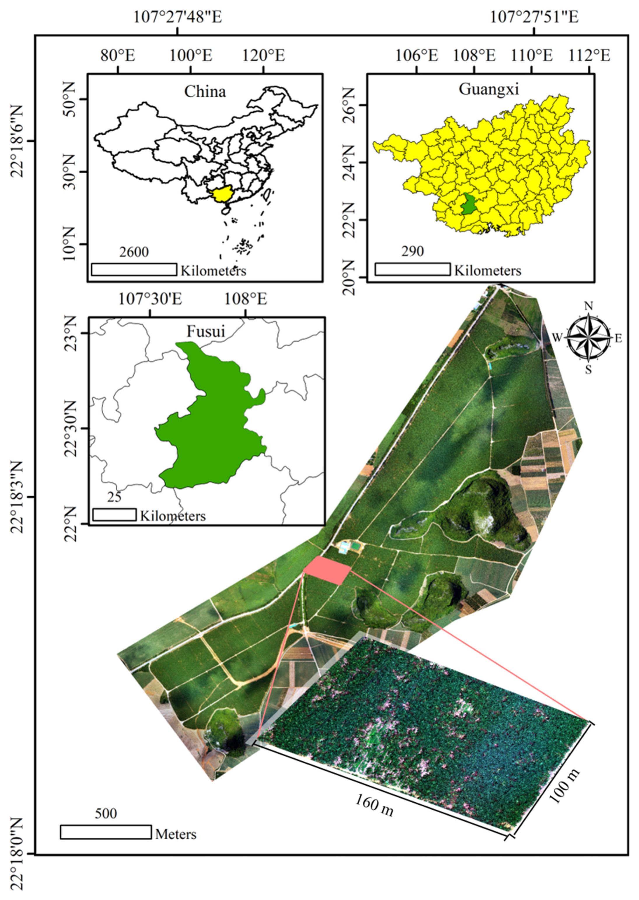
2.1. Study Area

Banana is the largest herbaceous flowering plant [21]. It is normally tall and fairly sturdy, often mistaken for trees. However, what appears to be a trunk is actually a pseudo-stem, which is formed by the tightly packed leaf sheaths. All the above-ground parts grow from a corm in the soil (Figure 1A). The flower emerges out from the center of the pseudo-stem right after the last leaf. The mother plant will wither after the banana is harvested, but the offshoots or suckers will grow up and continue to produce fruits next year [22]. Farmers usually keep 1–2 banana suckers for the coming year or generation, and the canopy of the mother plant will be chopped off to make the remaining nutrition in the pseudo-stem feeding the suckers [23].

A commercial banana plantation located in Fusui County, Guangxi Zhuang Autonomous Region, China (22°18′0.74″N, 107°27′50.1″E) (Figure 2) was studied. In the middle and late 2018, banana seedlings of the variety “Williams B6” (Musa AAA) were planted with a seedling distance and row distance of 2.5 m. The growth height of the variety is 3–5 m, and the growth cycle is 10–12 months. The planting density was about 1600 plants/ha, with an annual yield of about 54,420 kg/ha in 2019. BFW disease (Figure 1B–D) was spotted in 2019. To make up for the vacancies caused by the removal of infected banana plants, the growers started to retain two suckers for some of the healthy banana plants. Double suckers should increase the planting density and yield to a certain extent. However, due to the rapid spread of BFW disease, the number of the existing banana was only increased to 2070 plants/ha in 2020, with the annual yield decreased to 49,495 kg/ha. A field that was 160 m by 100 m in size was comprehensively investigated. The field had about 3300 existing banana plants and 352 vacancies caused by serious infection at the time of 14 July 2020. The site location and the study area are shown in Figure 2.

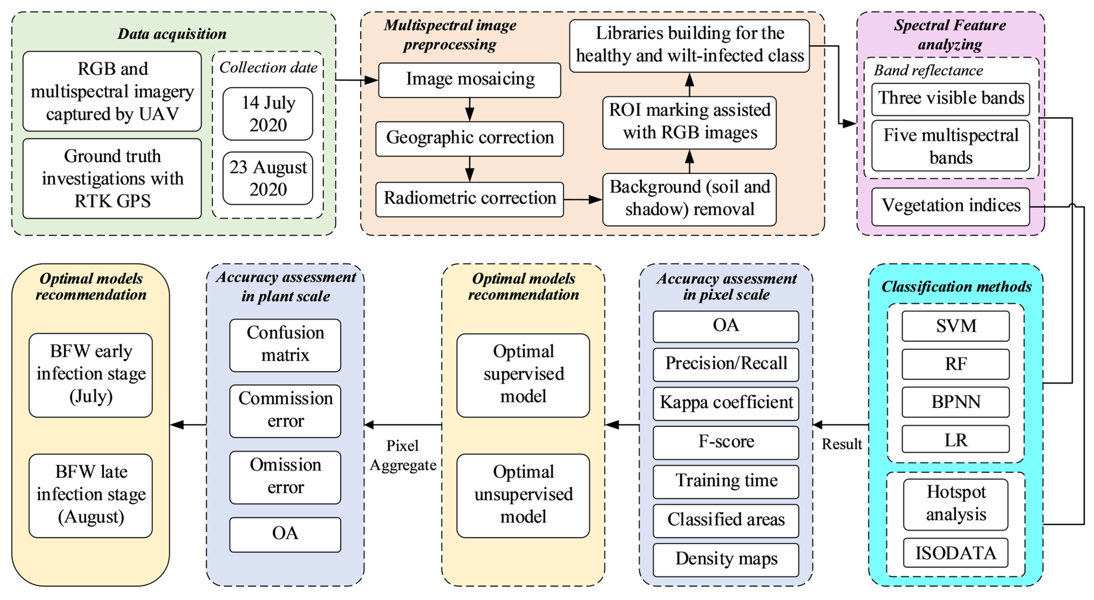
2.2. Overall Workflow

The technical route of this study is shown in Figure 3, including data acquisition, multispectral image preprocessing, spectral feature analyzing, establishment of supervised classification models based on band reflectance, establishment of unsupervised classification models based on VIs, accuracy assessment in pixel and plant scale. Optimal models were recommended for different kinds of classification methods and for different stages.

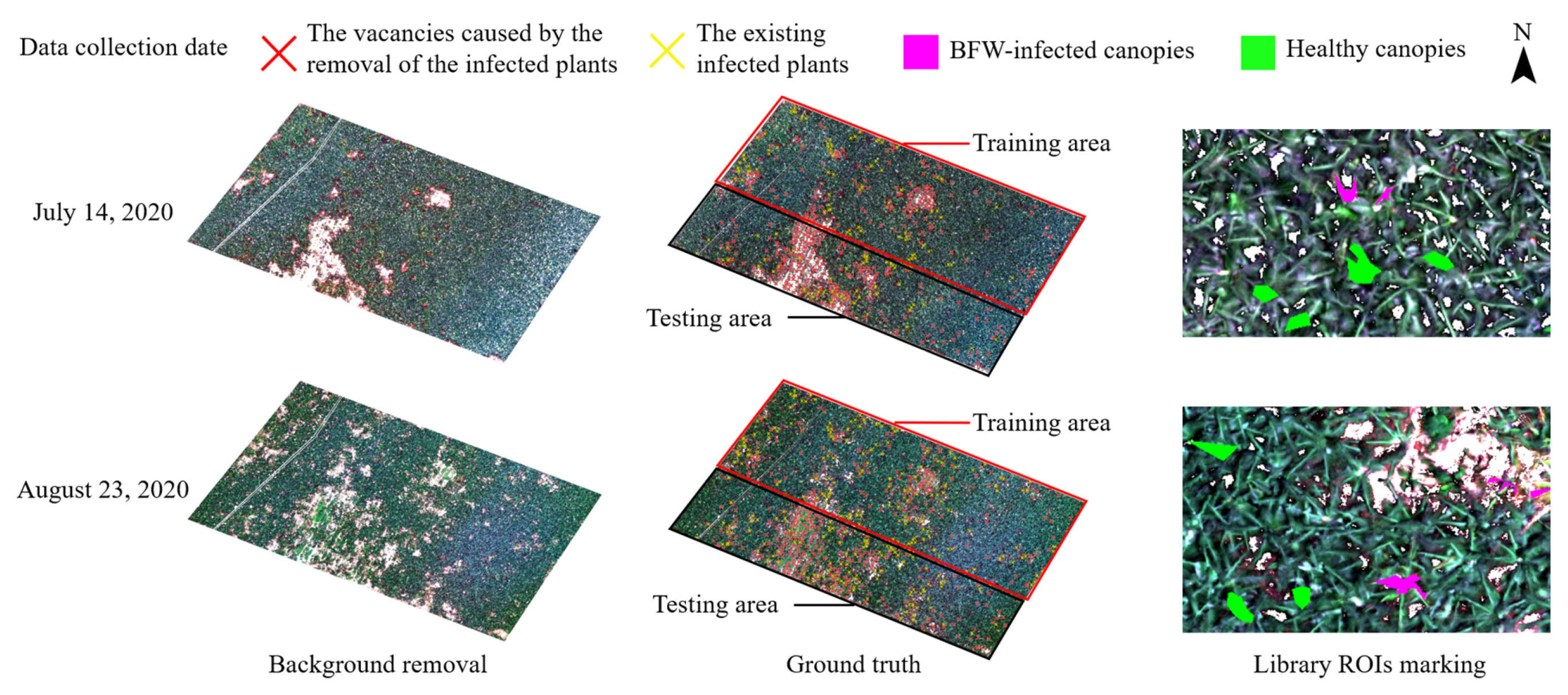
2.3. Data Acquisition

A drone (DJI Matrice 210 V2) equipped with a RedEdge MX (Micasense, Seattle, WA, USA) multispectral sensor and a Zenmuse X7 (DJI, Shenzhen, China) RGB sensor was used to acquire the canopy images (Figure 4a–c). RedEdge MX has five spectral acquisition channels: 475 ± 10 nm (blue, B), 560 ± 10 nm (green, G), 668 ± 5 nm (red, R), 717 ± 5 nm (red edge, RE), and 840 ± 20 nm (near-infrared, NIR), with a field view of 47.2° and an image resolution of 1280 × 960 pixels. It has two accessories including a light intensity sensor, which is used to correct the external light change. Zenmuse X7 is a compact camera with an integrated gimbal. It has 24 mm prime lenses, which can capture RGB images with a resolution of 6016 × 3376 pixels. During the data collection, both multispectral camera and RGB camera had their lens vertically downward. Four calibration tarps (Figure 4d) with reflectance of 5%, 20%, 40%, and 60% used for radiometric calibration were placed at the open place besides the field during the flights. Four red plates in 0.2 m × 0.2 m were also placed at the corners of the field as the ground control points (GCPs). Two flights were acquired on 14 July and 23 August 2020, with sunny, windless, and cloudless weather. Both flights had a flight height of 60 m and a flight speed of 4.5 m/s. Both the forward and side overlap were set to 85% in two flights. The ground sample distances (GSDs) of the multispectral images and the RGB images at the height of 60 m were 42.9 mm and 9.8 mm, respectively. About 285 multispectral images (including five bands for each multispectral image) and RGB images were collected for each flight.

Ground truth investigations were comprehensively conducted on the same day of the two flights. The infection status of all the banana plants were assessed by experienced farmers. BFW starts from the root and will gradually infect the leaves upward, the infected leaves will show obvious symptoms of yellowing and even withering. Plants with yellowish areas of more than 10% in canopy leaves were considered as diseased, while others were considered as healthy. A total of 352 vacancies and 139 existing infected plants were identified in the first ground survey on 14 July, and 158 new vacancies and 146 infected plants were found in the second ground survey on 23 August. Most of the vacancies were the infected plants in the first ground survey. The GPS coordinates of all the infected plants and vacancies, as well as the ground control points, were accurately recorded using a Real-time kinematic (RTK) positioning system, with the coordinate system of GCS_WGS_1984, UTM_Zone_48N.

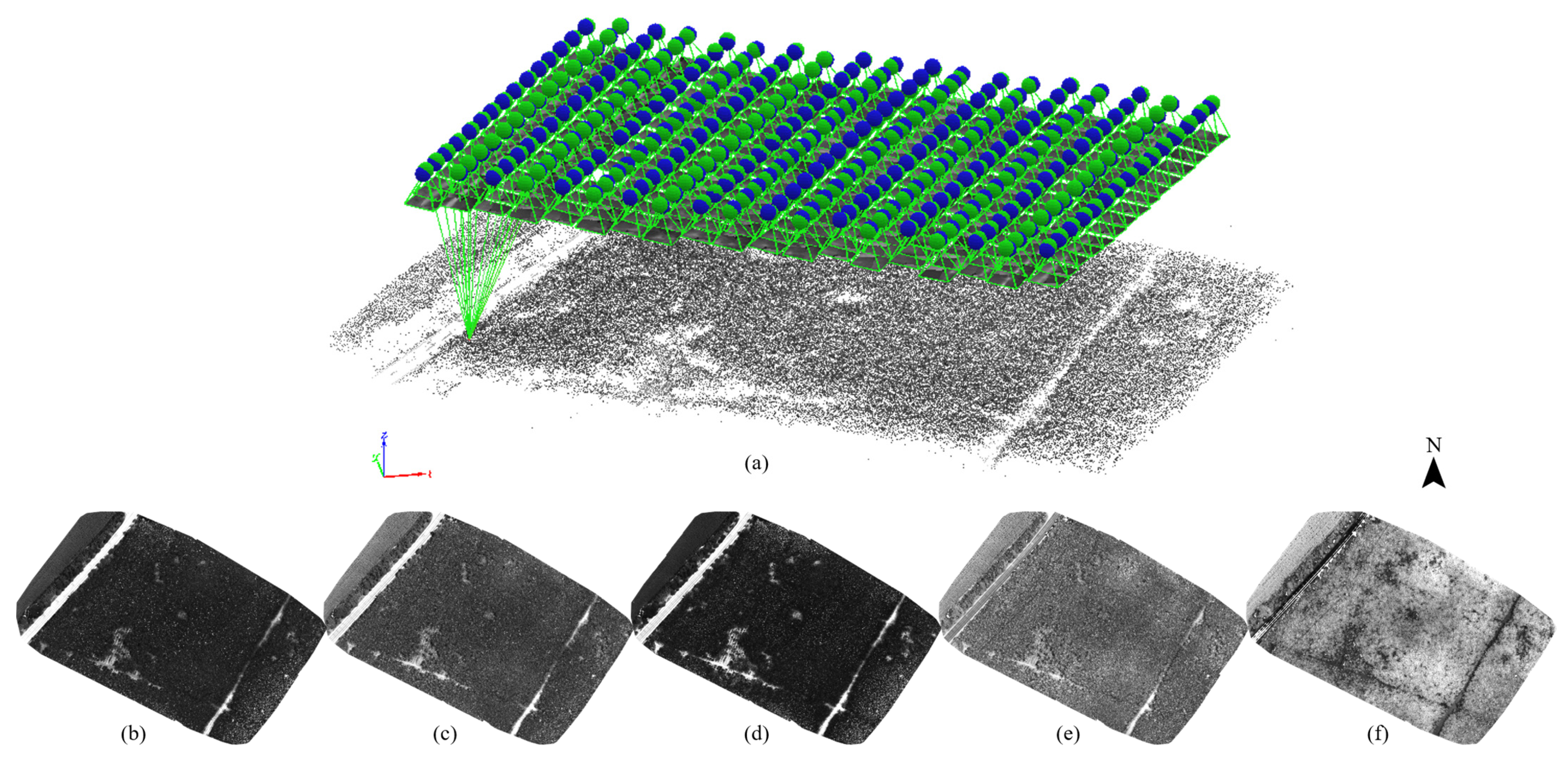
2.4. Data Preprocessing

Pix4DMapper (Pix4D, Prilly, Switzerland) was used to generate the mosaic image for each flight (shown in Figure 5). The 285 raw multispectral images with total size of 3.27 GB were imported into Pix4DMapper. By using the principles of photogrammetry and multi-eye reconstruction, the point cloud data were extracted from the multispectral images and feature registration was then performed to mosaic all the images. The digital orthophoto map (DOM) for each band was finally yielded. The size of the mosaiced multispectral image was reduced to 404 MB.

ENVI 5.5 (L3Harris Technologies, Melbourne, FL, USA) and ArcGIS 10.7 (ESRI, Redlands, CA, USA) were then used to implement radiometric correction, geographic correction, cropping, background removal, library building, etc. The processed mosaic images and the ground truth of the two flights are shown in Figure 6.

The method of “Empirical Line” in ENVI was selected to implement radiometric calibration since four calibration tarps with known reflectance were captured in the images [24]. First, the average DN values of the four calibration tarps were extracted for each band; then, linear regression was used to fit the DN values to the standard reflectance of the tarps; finally, all DN values were converted to reflectance with the fitted model.

The geometric correction was conducted using the “Image to Map” function based on the information of the four GCPs (at least three GSPs are required) [25]. The locations of the GCPs were firstly marked out on the image, and their corresponding coordinates recorded (in GCS_WGS_1984) in the field experiments were then imported. A first-order polynomial transformation method was selected as the correction model, “Nearest Neighbor” which could avoid introducing new pixel values, and was adopted for image resampling. The coordinate system was eventually reset to GCS_WGS_1984, UTM_Zone_48N, the same coordinate system used in the ground investigation. The geometric correction errors were 0.3217 pixels in July and 0.3314 pixels in August.

To implement better classification, the background such as the exposed soil and the shadow were firstly masked out by RF method. After mosaicing, radiometric correction, geometric correction, cropping, and background removal, the size of the preprocessed mosaiced multispectral image was further reduced from its original size of 404 MB to about 350 MB.

Building proper libraries for the healthy and BFW-infected classes was crucial for the supervised classification methods. In this study, library ROIs of the healthy and infected canopies were manually annotated based on the ground investigation coordinates and the color information of the RGB images. The infected banana plants have obvious yellowish symptoms in leaves, so the canopy areas with visible symptoms of the infected plants were marked out in irregular polygon shapes, forming the BFW-infected library. The healthy library was generated by randomly marking out the canopy areas of the healthy plants in irregular polygon shapes. The study field was then divided into a training and a testing area in a ratio of 2:1. The basic information of the training and testing set for both flights are shown in Figure 6 and

Table 1. Sample information of the training and testing sets.

Dataset	Classes	14 July 2020		23 August 2020
		Sample Plants	Sample Pixels/Pixel	Sample Plants	Sample Pixels/Pixel
Training set	BFW-infected	96	21,644	98	62,507
	Healthy	84	23,901	95	61,923
Testing set	BFW-infected	43	16,803	48	32,035
	Healthy	55	13,966	51	32,501

.

2.5. VIs

VI is a single value transformed from the observations (normally the reflectance values) of two or more spectral bands. It is used to enhance the contribution of vegetation features and thus allow reliable spatial and temporal inter-comparisons of terrestrial photosynthetic activity and canopy structural variations [26].

Twelve VIs were adopted as the input of the unsupervised models, as listed in

Table 2. Selected VIs and their calculation formulas.

VIs	Calculation Formula	References
Normalized Difference Vegetation Index (NDVI)	$NDVI=\left(NIR-R\right)/\left(NIR+R\right)$	[28]
Soil Adjusted Vegetation Index (SAVI)	$SAVI=1.5\ast \left(NIR-R\right)/\left(NIR+R+0.5\right)$	[29]
Renormalized Difference Vegetation Index (RDVI)	$RDVI=\left(NIR-R\right)/\sqrt{NIR+R}$	[30]
Wide Dynamic Range Vegetation Index (WDRVI)	$WDRVI=\left(0.2\ast NIR-R\right)/\left(0.2\ast NIR+R\right)$	[31]
Transformed Difference Vegetation Index (TDVI)	$TDVI=1.5\ast \left(NIR-R\right)/\sqrt{NI{R}^2+R+0.5}$	[32]
Simple Ratio Index (SRI)	$SRI=NIR/R$	[33]
Modified Simple Ratio Index (MSRI)	$MSRI=\left(NIR/R-1\right)/\left(\sqrt{NIR/R}+1\right)$	[34]
Non-Linear Index (NLI)	$NLI=\left(NI{R}^2-R\right)/\left(NI{R}^2+R\right)$	[35]
Modified Non-Linear Index (MNLI)	$MNLI=1.5\ast \left(NI{R}^2-R\right)/\left(NI{R}^2+R+0.5\right)$	[36]
Green Difference Vegetation Index (GDVI)	$GDVI=NIR-G$	[37]
Anthocyanin Reflectance Index 1 (ARI1)	$ARI1=1/G-1/RE$	[38]
Anthocyanin Reflectance Index 2 (ARI2)	$ARI2=NIR\ast \left(1/G-1/RE\right)$	[38]

Note: B, G, R, RE and NIR represent the spectral reflectance at 475 ± 10 nm (blue), 560 ± 10 nm (green), 668 ± 5 nm (red), 717 ± 5 nm (red edge), and 840 ± 20 nm (near infrared) respectively.

. Since healthier vegetation absorbs more visible light while reflecting most of the NIR light [27], VIs derived from the reflectance in red, green, and NIR range were prioritized such as NDVI, SAVI, RDVI, WDRVI, SRI, MSRI, GDVI, etc.

NDVI, which is based on spectral reflectance in the red and NIR range, has high correlation with the photosynthetic activity or vigor of the plant, and it is considered as one of the most common indices used to predict crop growth status and nutrition information [28]. However, it can be affected by some environmental factors such as soil and dense vegetation. Soil Adjusted Vegetation Index (SAVI) and Renormalized Difference Vegetation Index (RDVI) are similar to NDVI, as they are usually used to monitor vegetation coverage and water stress, but SAVI can minimize the effects of soil pixels [29] and performs better in sparsely vegetated areas; while RDVI is sensitive to healthy vegetation and insensitive to soil and solar geometry [30]. Wide Dynamic Range Vegetation Index (WDRVI), which is also similar to NDVI, can quantify the biophysical characteristics of crops and enable dynamic monitoring of crop growth status; however, WDRVI is more sensitive to a wider range of vegetation fractions [31]. Transformed Difference Vegetation Index (TDVI) is commonly used to monitor vegetation cover as it has linear relationship to vegetation cover [32], and it does not saturate like NDVI or SAVI. Simple Ratio Index (SRI), which is one of the most easy-calculated indices, is the ratio of the wavelength with the highest reflectivity in the NIR range to the wavelength with the deepest chlorophyll absorption in the visible range, but its sensitivity will be reduced in dense vegetation [33]. It also has a mathematically infinite range (0 to infinity), which can be a practical disadvantage as compared to the normalized VIs. Modified Simple Ratio Index (MSRI) increases the sensitivity to vegetation biophysical parameters by combining SR into the RDVI formula and is commonly used to estimate leaf area indices [34]. With the assumption that the relationship between many VIs and surface biophysical parameters is non-linear, Non-Linear Index (NLI) could linearize the relationship with surface parameters that tend to be non-linear [35]. Modified Non-Linear Index (MNLI) is an enhancement to NLI that incorporates SAVI to account for the soil background [36]. NLI and MNLI are both useful to estimate biophysical information. Green Difference Vegetation Index (GDVI) is based on the green and NIR band and is more sensitive to leaf water content and chlorophyll content, so it was usually used to monitor the photosynthetically active biomass of vegetation [37] as well as nitrogen requirements. Anthocyanin Reflectance Index 1 (ARI1) is based on the green and RE range, and very sensitive to anthocyanins in leaves [38]. Increasing in ARI1 indicates canopy change in foliage via new growth or death. Anthocyanin Reflectance Index 2 (ARI2) is a refinement of ARI1 which includes one more band reflectance in NIR range, and is more effective when anthocyanin concentrations are high [38].

2.6. Classification Methods

Four supervised methods named SVM, RF, BPNN, and LR, and two unsupervised methods named HA and ISODATA were used to classify the healthy and BFW-infected canopies in pixel scale [39]. The supervised classification methods were first trained in the training area and then evaluated in the testing area. As unsupervised methods do not require training, they were directly implemented on the entire area.

2.6.1. SVM

SVM is derived from statistical learning theory [40]. It maps data from a low-dimensional space to a high-dimensional space through a kernel function and separates the classes with a decision surface that maximizes the margin between the classes. In this study, the Radial Basis Function (RBF) kernel was used, the convergence criterion was set to 0.00001, and the maximum number of iterations is 100.

2.6.2. RF

RF integrates multiple trees through the idea of ensemble learning. From an intuitive point of view, each decision tree is a classifier. For input samples, N trees will have N classification results [41]. The final classification results are determined by the majority voting of each decision tree. In this study, the RF model contained 100 trees, the split criterion was Gini impurity, the maximum depth of the tree was set to 4, the minimum number of samples required to split a node and the minimum number of samples for each leaf node were 2, and the feature number was set as the square root of the number of input image bands to be classified, which was 2, in this case.

2.6.3. BPNN

BPNN is a multi-layer feedforward network trained by the error inverse propagation algorithm [42]. It uses the error of the output layer to estimate the error of the previous layer and keeps feeding forward. In this way, the error is backpropagated through the network and weight adjustment is made using a recursive method. Eventually, the model is optimized and the non-linear classification is realized. The main parameters of the BPNN model were set as follows: the activation function was logistic; the minimum and maximum iteration times were 500 and 1000, respectively; the learning rate was 0.2, and the number of hidden layers was 2.

2.6.4. LR

LR is an important machine learning method that uses a similar regression method to solve the classification problem. Essentially, it used a logistic function to model a binary dependent variable [43]. The probability of a class is related to a set of explanatory variables, which is useful for explaining the classification phenomenon. The gradient descent trainer updates and optimizes the classifier according to the iterative gradient. The main parameters were set up as follows: the convergence criterion was 0.000001, the maximum iteration was 100, and the learning rate was 50.

2.6.5. ISODATA

ISODATA is one of the most famous variants of the K-means clustering algorithm [44]. In K-means, the number of clusters (K) needs to be artificially determined in advance and cannot be changed throughout the algorithm. By introducing dynamic criteria, which can adaptively remove or merge the classes with too few samples and divide the class with a large degree of dispersion, ISODATA solved this problem. The main parameters of the ISODATA model in this study were set up as follows: the input feature was VI, and the minimum pixels of a class was 30,000.

2.6.6. HA

HA groups neighboring pixels of similar value into clusters by calculating Getis–Ord G_i* local statistics [45]. It evaluates each pixel and its surrounding pixels within a specified distance to classify the pixel as “hot” or “cold” (statistically significant clusters of high or low values, respectively) or neutral (not statistically significant). HA can be used to look for variations throughout an area. The calculation of Getis–Ord G_i* is shown in Equations (1)–(3).

$$G_i^{*}=\frac{{\displaystyle \sum _{j=1}^n{w}_{ij}{x}_j}-\overline{X}{\displaystyle \sum _{j=1}^n{w}_{ij}}}{\sqrt[S]{\frac{\left[n{\displaystyle \sum _{j=1}^n{w}_{ij}^2}-{\left({\displaystyle \sum _{j=1}^n{w}_{ij}}\right)}^2\right]}{n-1}}}$$

(1)

$$\overline{X}=\frac{{\displaystyle \sum _{j=1}^n{x}_j}}{n}$$

(2)

$$S=\sqrt{\frac{{\displaystyle \sum _{j=1}^n{x}_j^2}}{n}-{\left(\overline{X}\right)}^2}$$

(3)

where $G_i^{*}$ is a z-score of patch i; x_j is the pattern value for patch j; w_ij is the spatial weight between patch i and patch j, if the distance from a neighbor j to the feature i is within the distance, w_ij = 1; otherwise w_ij = 0; n is the total number of grid cells.

The main parameters in this study were set up as follows: the input feature was VI, and the specified distance was 0.1 m.

2.7. Accuracy Assessment

Since only two classification classes, the healthy and BFW-infected, were defined, the descriptors of true positive (TP), false positive (FP), true negative (TN), and false negative (FN) were used to form the confusion matrix (Equation (4)) and thus to calculate the accuracy assessment parameters [11,46] such as OA (Equation (5)), precision (Equation (6)), recall (Equation (7)), Kappa coefficient (Equation (8)), and F-score (Equation (9)).

$$Confusion Matrix=\left[\begin{array}{cc}TP& FP\\ FN& TN\end{array}\right]$$

(4)

$$OA=\frac{TP+TN}{TP+TN+FP+FN}$$

(5)

$$Precison=\frac{TP}{TP+FP}$$

(6)

$$Recall=\frac{TP}{TP+FN}$$

(7)

$$Kappa\_coef=\frac{p_o-p_e}{1-p_e}$$

(8)

$$F\_score=\frac{2TP}{FP+2TP+FN}$$

(9)

where, p_o represents the OA, and p_e can be calculated by Equation (10).

$$p_e=\frac{(TP+FP)\times (TP+FN)+(FN+TN)\times (FP+TN)}{{(TP+TN+FP+FN)}^2}$$

(10)

3. Results

3.1. Spectral Feature Analyzing Results

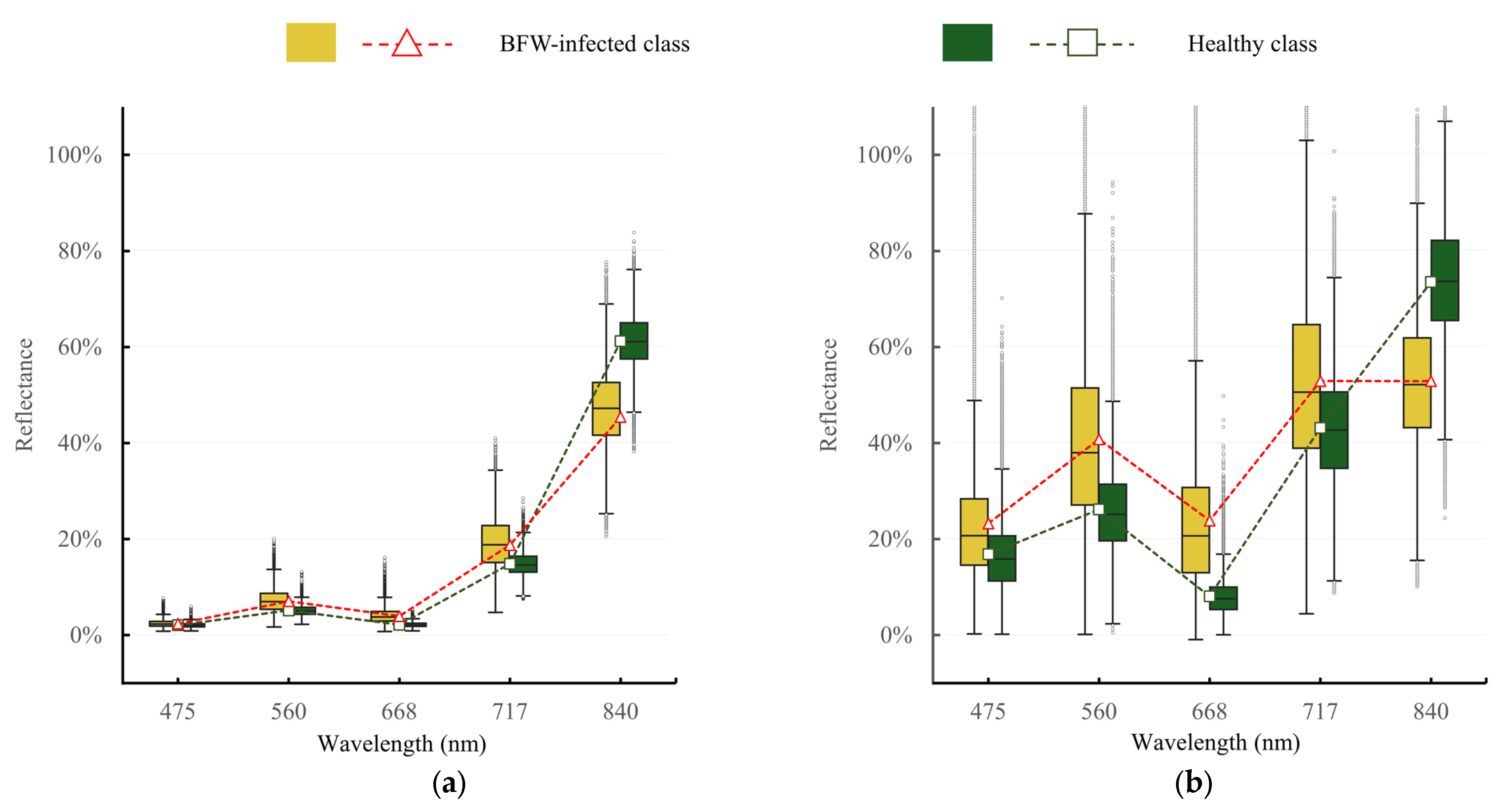
3.1.1. Reflectance Difference of the Healthy and BFW-Infected Canopies

The spectral reflectance between the healthy and BFW-infected libraries are shown in Figure 7. From the box plots, it can be seen that the boxes which represent the middle half of the datasets had small overlaps for most of the bands, especially for the red and NIR bands, indicating an obvious difference existed between the two classes, but the difference was much less obvious at blue and RE band. Moreover, the reflectance distribution of each band in August was wider than that in July, indicating that with the development of the disease, the spectral characteristics showed more variation. The average reflectance represented by the dashed lines tells a clearer difference between the two classes: the BFW-infected class had higher reflectance at the visible region, but lower reflectance at the NIR region than the healthy one.

3.1.2. Feature Analyzing of the Selected VIs

The histograms of the selected VIs of the healthy and BFW-infected classes are plotted in Figure 8. All VIs had obvious distribution differences between the two classes. The average value of the healthy class was significantly higher than that of the infected class. The first quantile of the healthy class, the third quantile of the infected class, and their ratio were calculated for quantitative comparison. The results showed that, except for ARI1, the quantile ratios were 100% to 150% in July, and 130% to 200% in August.

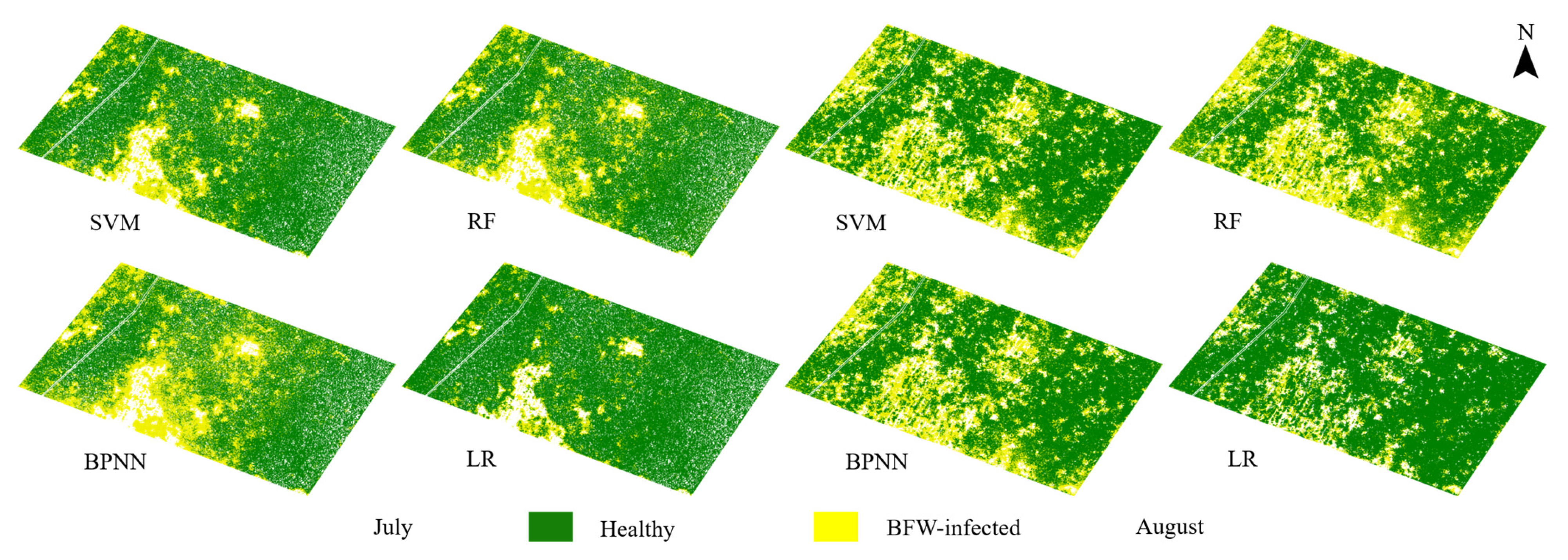
3.2. Classification Results of the Supervised Models Based on Band Reflectance

For the supervised methods, two kinds of images with different band combinations were adopted as the inputs, one was the three-visible-band (three-band) images including blue, green, and red; the other was the five-multispectral-band (five-band) images including blue, green, red, RE, and NIR. Taking the reflectance of the selected bands as the input, eight classification models were built for each flight. The classification results based on pixel scale are listed in

Table 3. Classification accuracies of the SVM, RF, BPNN, and LR models in pixel scale.

Flight Dates	Inputs	Classes	SVM			RF			BPNN			LR
			Precision /%	Recall /%	F-Score	Precision /%	Recall /%	F-Score	Precision /%	Recall /%	F-Score	Precision /%	Recall /%	F-Score
14 July 2020	Three-visible-band images	BFW-infected	99.07	90.61	0.95	96.80	92.73	0.95	95.51	95.30	0.95	99.96	79.27	0.88
		Healthy	89.55	98.95	0.94	91.50	96.23	0.94	94.37	94.61	0.94	79.70	99.96	0.89
		OA/%	94.35			94.30			94.99			88.56
		Kappa coefficient	0.89			0.89			0.90			0.77
	Five-multispectral-band images	BFW-infected	98.39	96.30	0.97	98.10	96.95	0.98	97.89	97.07	0.97	99.29	93.93	0.97
		Healthy	95.57	98.06	0.97	96.30	97.69	0.97	96.51	97.48	0.97	93.14	99.19	0.96
		OA/%	97.09			97.28			97.25			96.32
		Kappa coefficient	0.94			0.95			0.95			0.93
	Contribution of the RE and NIR bands in OA/%		2.74			2.98			2.26			7.76
23 August 2020	Three-visible-band images	BFW-infected	93.66	96.15	0.95	87.83	96.42	0.92	93.50	95.68	0.95	99.70	78.30	0.88
		Healthy	96.12	93.61	0.95	96.47	86.83	0.91	95.99	93.44	0.95	82.40	99.77	0.90
		OA/%	94.87			91.59			94.55			89.13
		Kappa coefficient	0.90			0.83			0.89			0.78
	Five-multispectral-band images	BFW-infected	95.95	98.12	0.97	95.95	97.37	0.97	95.64	97.71	0.97	98.08	95.04	0.97
		Healthy	98.11	95.94	0.97	97.72	95.95	0.97	98.04	95.61	0.97	95.27	98.17	0.97
		OA/%	97.02			96.66			96.65			96.62
		Kappa coefficient	0.94			0.93			0.93			0.93
	Contribution of the RE and NIR bands in OA/%		2.15			5.07			2.10			7.49

.

As can be seen in Table 3, the five-band images had higher OAs of more than 96% and higher Kappa coefficients of more than 0.93 than the three-band images which had OAs of more than 88% and Kappa coefficients of more than 0.77. SVM, RF, and BPNN had very similar results for both kinds of inputs in both flights; their OAs reached more than 96% for the five-band images and more than 91% for the three-band images. LR had significantly lower accuracies, especially for the three-band images, with an OA of about 89%.

The training times of all the methods are listed in

Table 4. Training times of the SVM, RF, BPNN, and LR models based on the multispectral image.

Classifier	Training Time Based on the Five-Band Images/min
SVM	245
RF	22
BPNN	31
LR	2

. SVM, which had the highest OA, also had the longest training time of 245 min under the computer capacity of Inter Core i9-9900X CPU, NVIDIA GeForce RTX 2080 Ti GPU, and 64 GB RAM. BPNN and RF had much shorter training times than SVM, but with similar OA. LR had the shortest training time of 2 min, but with obvious lower accuracy.

The classification maps of those supervised models are also exhibited in Figure 9 and Figure 10. The yellow color represents the BFW-infected class, and the green represents the healthy class. It can be seen that SVM, RF, BPNN, and LR yielded very similar distribution maps based on the five-band images (Figure 10), but not for the three-band images. LR recognized much less infection pixels comparing to other methods under the same period. BPNN recognized slightly more infection pixels in July. On the whole, the five-band models identified more diseased pixels (Figure 10) than the three-band models (Figure 9) in both July and August, especially in July.

The classified pixel numbers and areas based on the five-band images were further counted, as shown in

Table 5. Areas of each class classified by the SVM, RF, BPNN, and LR classifiers based on the five-multispectral-band images.

Classifier	Classes	14 July 2020			23 August 2020
		Sample Pixels /Pixel	Area/Ha	Percentage of the Studied Area/%	Sample Pixels /Pixel	Area/Ha	Percentage of the Studies Area/%
SVM	BFW-infected	2,780,478	0.53	33.13	2,724,278	0.52	32.50
	Healthy	4,336,422	0.83	51.88	4,810,415	0.91	56.88
RF	BFW-infected	2,798,059	0.53	33.13	2,685,407	0.51	31.88
	Healthy	4,374,251	0.83	51.88	4,849,286	0.92	57.50
BPNN	BFW-infected	3,114,152	0.59	36.88	2,800,873	0.53	33.13
	Healthy	4,058,158	0.77	48.13	4,733,820	0.90	56.25
LR	BFW-infected	2,359,306	0.45	28.13	2,282,519	0.43	26.88
	Healthy	4,757,502	0.91	56.88	5,252,174	1.00	62.50

. All methods produced larger areas of infection in July than in August. SVM and RF recognized similar areas of infection of about 33% of the studied area in July and 32% in August; BPNN had a slightly larger area of infection of 36.88% in July and 33.13% in August, and LR had much smaller areas of infection of 28.13% in July and 26.88% in August, showing that BPNN and LR yielded results with large differences. The results reflect that SVM and RF had more stable results.

To make a more intuitive evaluation of the classification performance, the true density maps were generated in ArcGIS with the spatial kernel density analyst method [47]. The density features were calculated according to the spatial relationship of disease distributions within a neighborhood. The infected pixels classified by the SVM and RF models based on the five-band images were overlaid on the true density maps, as shown in Figure 11. The classified infected pixels were mainly concentrated in the severely infected areas, showing high consistent distributions with the ground truth.

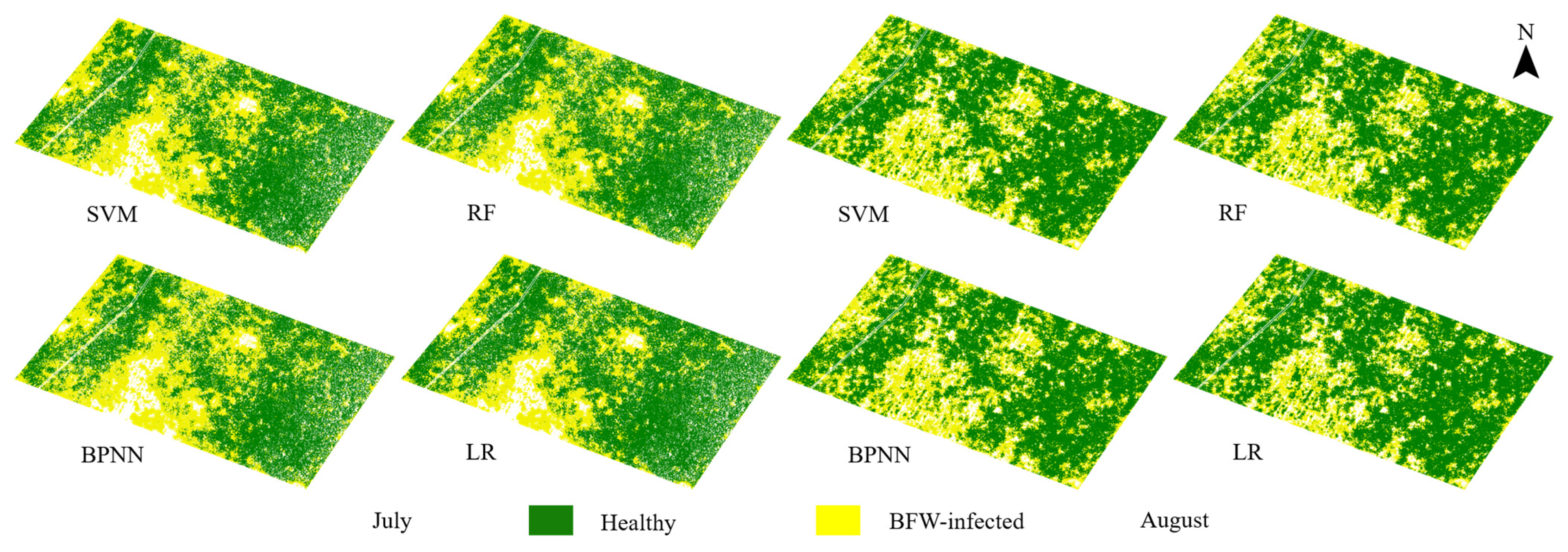
3.3. Classification Results of the Unsupervised Models Based on Different VIs

3.3.1. Classification Results of the HA Models

HA generally processes data within single matrix. In this case, only one band of information was needed as the input. To better utilize the multiple-band information, VIs which were generated from the reflectance of multiple bands were chosen as the input for HA.

The classification results of HA based on various VIs are shown in

Table 6. Classification accuracies in pixel scale of HA based on different VIs.

Inputs	Classes	14 July 2020					23 August 2020
		Precision/%	Recall/%	F-Score	OA/%	Kappa Coefficient	Precision/%	Recall/%	F-Score	OA/%	Kappa Coefficient
MSRI	BFW-infected	99.04	96.18	0.98	97.58	0.95	94.23	94.49	0.94	94.28	0.89
	Healthy	96.15	99.03	0.98			94.63	94.07	0.94
SRI	BFW-infected	98.48	96.66	0.98	97.54	0.95	96.86	94.72	0.96	95.81	0.92
	Healthy	96.60	98.45	0.98			94.80	96.91	0.96
WDRVI	BFW-infected	99.84	94.24	0.97	96.99	0.94	95.47	94.84	0.95	95.14	0.90
	Healthy	94.36	99.84	0.97			95.03	95.45	0.95
NDVI	BFW-infected	99.96	92.86	0.96	96.34	0.93	98.40	92.67	0.95	95.55	0.91
	Healthy	93.10	99.96	0.96			93.20	98.45	0.96
TDVI	BFW-infected	99.96	92.68	0.96	96.25	0.93	98.75	91.94	0.95	95.36	0.91
	Healthy	92.94	99.96	0.96			92.59	98.80	0.96
GDVI	BFW-infected	98.95	83.30	0.90	91.05	0.82	98.48	96.01	0.97	97.24	0.95
	Healthy	85.12	99.09	0.92			96.27	98.49	0.97
RDVI	BFW-infected	99.22	94.04	0.97	91.54	0.83	99.65	92.72	0.96	96.17	0.92
	Healthy	85.72	99.32	0.92			93.33	99.65	0.96
SAVI	BFW-infected	99.31	83.47	0.91	91.29	0.83	99.68	92.76	0.96	96.21	0.92
	Healthy	85.29	99.39	0.92			93.36	99.68	0.96
NLI	BFW-infected	100.00	86.86	0.93	93.31	0.87	99.70	91.80	0.96	95.73	0.92
	Healthy	88.01	100.00	0.94			92.53	99.69	0.96
MNLI	BFW-infected	99.03	82.66	0.90	90.76	0.82	99.23	91.96	0.95	95.60	0.91
	Healthy	84.65	99.16	0.91			92.64	99.26	0.96
ARI2	BFW-infected	91.49	95.46	0.93	93.17	0.86	80.41	93.84	0.87	85.43	0.71
	Healthy	95.07	90.80	0.93			92.77	76.96	0.84
ARI1	BFW-infected	62.97	82.91	0.72	66.48	0.33	63.91	85.53	0.73	68.50	0.37
	Healthy	65.67	38.18	0.48			84.03	74.26	0.79

. Most VIs had higher OA than 90%; MSRI, SRI, WDRVI, NDVI, TDVI, and GDVI had the best classification performance with the OA higher than 94% for both flights, but ARI1 had obviously poor performance with an OA less than 70%. MSRI had the highest accuracy (OA = 97.58%) in July, but relatively lower accuracy (OA = 94.28%) in August; GDVI had the highest accuracy (OA = 97.24%) in August, but relatively lower accuracy (OA = 91.05%) in July. Some VIs such as SRI and ARI2 had abnormal values due to the residual background, which could cause classification failure of HA, so an extra process of outlier elimination was implemented on those VIs to ensure successful classification.

Without sampling or training, HA only required about 18 s to generate the classification result for a VI image with a size of 88 MB, which was significantly faster than the supervised methods. However, similar classification results could be obtained only if appropriate VI was chosen.

Figure 12 shows the classification maps of the HA models based on MSRI, WDRVI, NDVI, and GDVI. The yellow pixels represented “cold” pixels which had lower z-scores in G_i* statistics; the green represented “hot” which had higher z-scores. In general, the distribution trends of the identification results of each vegetation index were very close.

The classified pixel quantities and the corresponding areas of the HA models based on the four VIs are also listed in

Table 7. Areas of each class classified by the HA models based on VIs.

Inputs	Classes	14 July 2020			23 August 2020
		Sample Pixels /Pixel	Area/Ha	Percentage of Study Area/%	Sample Pixels /Pixel	Area/Ha	Percentage of Study Area/%
MSRI	BFW-infected	2,284,183	0.43	26.88	2,563,659	0.49	30.63
	Healthy	4,888,127	0.93	58.13	4,965,306	0.94	58.75
WDRVI	BFW-infected	1,797,986	0.34	21.25	2,525,353	0.48	30.00
	Healthy	5,374,324	1.02	63.75	5,009,340	0.95	59.38
NDVI	BFW-infected	1,612,276	0.31	19.38	2,080,738	0.39	24.38
	Healthy	5,560,034	1.05	65.63	5,453,955	1.04	65.00
GDVI	BFW-infected	2,549,798	0.48	30.00	2,853,141	0.54	33.75
	Healthy	4,622,512	0.88	55.00	4,681,552	0.89	55.63

. The classified infected areas in August were all larger than that in July for all the models. But the infected areas had certain fluctuation (19.38%–30.00% in July, 24.38%–33.75% in August).

The identified BFW-infected pixels by the HA models were overlaid on the true density maps as well; MSRI and GDVI were selected to demonstrate the results, as shown in Figure 13. On the whole, the identified BFW-infected pixels were also highly consistent with the ground truth for both VIs in the two periods. However, looking closely to the zone with infected density of “0–10 infected plants per 100 m²”, more infected pixels were detected based on GDVI in July and MSRI in August, which meant a high possibility of misclassification, and thus it supported that GDVI had lower OA than MSRI in July, but higher OA in August.

3.3.2. Comparison of Results between the HA Models and the ISODATA Models

HA reached good accuracy performance based on most of the Vis; in order to further determine the main reason (the classification method or the input VI of the model) for the good performance, another unsupervised method—ISODATA was used to compare with HA. Four VIs (MSRI, WDRVI, NDVI, and GDVI) which had wider differences between BWF-infected and healthy canopies were demonstrated in the model comparison. The results are shown in

Table 8. Classification accuracies in pixel scale of the HA and ISODATA models based on MSRI, WDRVI, NDVI, and GDVI.

Methods	VI	Classes	14 July 2020				23 August 2020
			Precision/%	Recall/%	OA/%	Kappa Coefficient	Precision/%	Recall/%	OA/%	Kappa Coefficient
HA	MSRI	BFW-infected	99.02	96.72	97.86	0.96	94.23	94.49	94.28	0.89
		Healthy	96.74	99.02			94.63	94.07
	WDRVI	BFW-infected	99.84	94.24	96.99	0.94	95.47	94.84	95.14	0.90
		Healthy	94.36	99.84			95.03	95.45
	NDVI	BFW-infected	99.96	93.33	96.61	0.93	98.40	92.67	95.55	0.91
		Healthy	93.64	99.96			93.20	98.45
	GDVI	BFW-infected	99.12	82.91	91.01	0.82	98.48	96.01	97.24	0.95
		Healthy	85.08	99.25			96.27	98.49
	Average OAs				95.62				95.55
ISODATA	MSRI	BFW-infected	99.73	3.13	53.21	0.03	80.04	67.18	75.13	0.50
		Healthy	52.49	99.99			71.56	83.14
	WDRVI	BFW-infected	100.00	0.02	49.13	0.0002	99.93	37.98	67.33	0.37
		Healthy	49.12	100.00			59.18	99.97
	NDVI	BFW-infected	100.00	0.20	51.84	0.003	99.60	63.67	81.65	0.63
		Healthy	51.84	99.99			74.17	99.74
	GDVI	BFW-infected	99.62	2.25	52.78	0.02	61.79	99.97	69.18	0.39
		Healthy	52.27	99.99			99.92	38.60
	Average OAs				51.74				73.32

. As can be seen, the average OAs of HA reached more than 95% both in July and August, and the average OAs of ISODATA only reached 51.74% in July, and 73.32% in August, which were 43.88% and 22.23% less than that of HA. This result of ISODATA had higher OA in August which again proved that the late infection stage had more obvious spectral features and was easier to be classified with unsupervised methods.

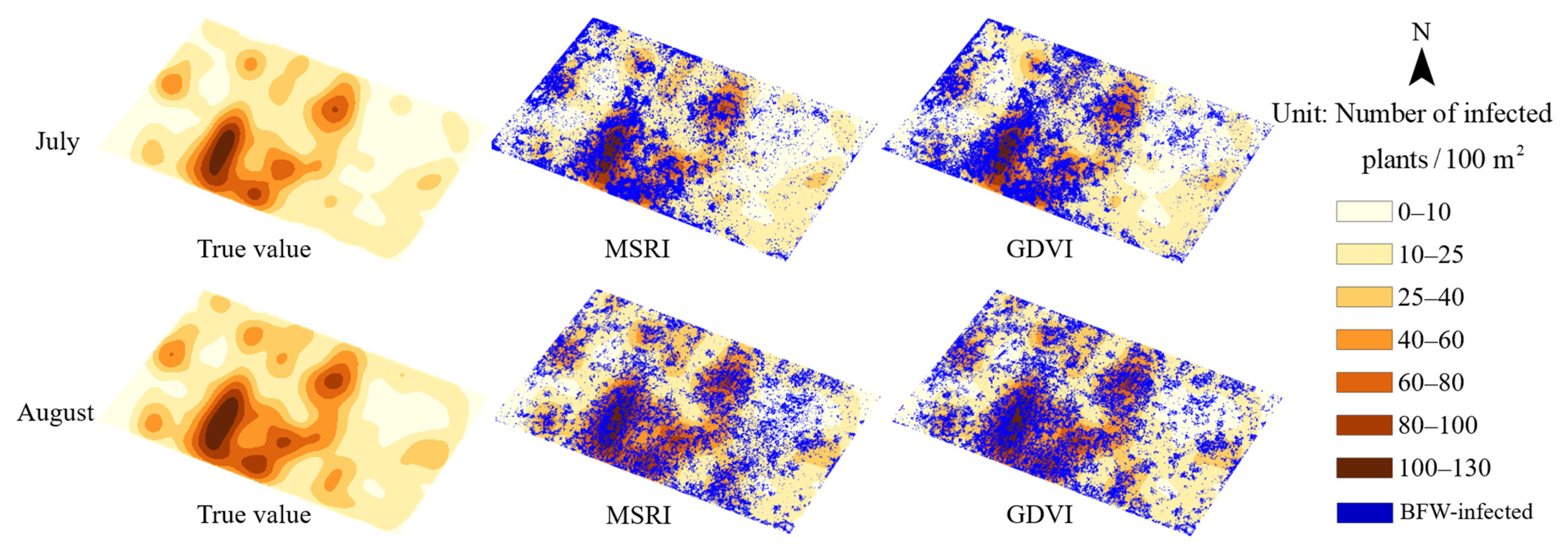
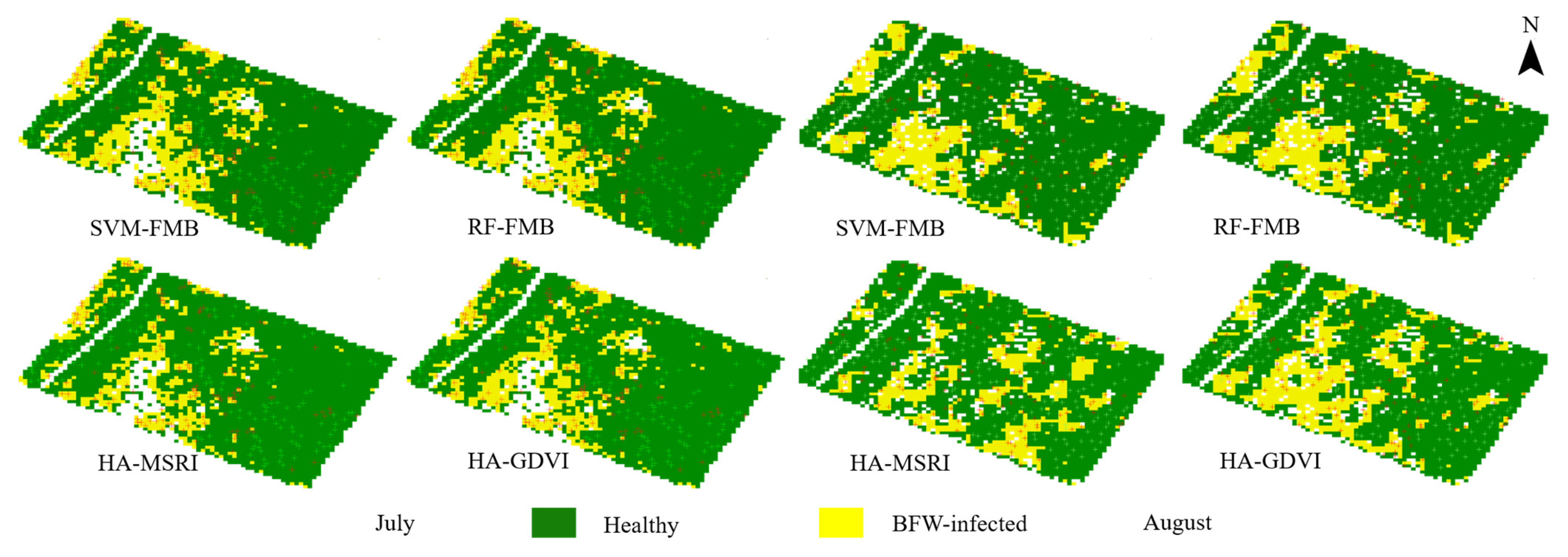
3.4. Classification Results in Plant Scale

The previous results were evaluated in pixel scale. Banana is a tree-like herb with broad leaves; a plant occupies an average area of about 2.5 m × 2.5 m, containing about 4500 pixels in the multispectral images. In addition, the diseased area of each infected plant was varied, which made it difficult to determine the plant-based recognition accuracy. Some studies yielded the plant-based classification results by first locating the individual plant and then diagnosing its infection status [1]. However, the plants in this study were too dense to separate correctly. Therefore, a resampling method named Pixel Aggregation was adopted to resize the pixel-based results to plant scale. It was used to resize the pixel-based classification images of 5103 × 3166 pixels to plant-based images of 86 × 78 pixels.

The resampled results of several representative models are shown in Figure 14 and

Table 9. The classification accuracies in plant scale.

Models		Classes	14 July 2020					23 August 2020
			Ground Truth		Commission Error /%	Omission Error /%	OA/%	Ground Truth		Commission Error /%	Omission Error /%	OA/%
			BFW Infected	Healthy				BFW Infected	Healthy
Supervised methods	SVM	BFW-infected	124	0	0.00	10.79	94.60	123	0	0.00	15.75	92.12
		Healthy	15	139	9.74	0.00		23	146	13.61	0.00
	RF	BFW-infected	120	0	0.00	13.67	93.17	123	0	0.00	15.75	92.12
		Healthy	19	139	12.03	0.00		23	146	13.61	0.00
	BPNN	BFW-infected	123	0	0.00	11.51	94.24	123	0	0.00	15.75	92.12
		Healthy	16	139	10.32	0.00		23	146	13.61	0.00
	Average OAs						94.00					92.12
HA	MSRI	BFW-infected	118	0	0.00	15.11	92.45	132	0	0.00	9.59	95.21
		Healthy	21	139	13.13	0.00		14	146	8.75	0.00
	WDRVI	BFW-infected	108	0	0.00	22.30	88.85	131	0	0.00	10.27	94.86
		Healthy	31	139	18.24	0.00		15	146	9.32	0.00
	NDVI	BFW-infected	104	0	0.00	25.18	87.41	120	0	0.00	17.81	91.10
		Healthy	35	139	20.11	0.00		26	146	15.12	0.00
	GDVI	BFW-infected	119	0	0.00	14.39	92.81	131	0	0.00	10.27	94.86
		Healthy	20	139	12.58	0.00		15	146	9.32	0.00
	Average OAs						90.38					94.01

. In Figure 14, one colored pixel represented one banana plant; the red crosses and the green crosses represented the true infected plants and the randomly selected healthy plants for library building. The crosses which were located one more pixel away from the nearest pixels of the corresponding class were considered as omission samples.

All the listed models had relatively lower OA (about 3% less) in Table 9 than the pixel-based results in Table 3, Table 4, Table 5 and Table 6. The omission errors of the healthy class and the commission errors of the infected class were 0 for all the models, which means all the healthy samples were correctly identified and no healthy samples were misclassified as infected ones. However, it can be seen from Figure 14, that some healthy plants which were not marked out in green crosses were misclassified as infected ones, which seems to contradict with the result in Table 9. That is because only the healthy samples selected for library building were counted in Table 9. However, looking closely at Figure 14, the misclassified infected samples were mainly located around the open areas near vacancies or infected plants, the ground surface of where was mostly covered with the residuals of infected plants. Those residuals had similar spectral features with the infected canopies and were hard to be totally masked out in the procedure of background removal. This kind of misclassification caused little influence on the identification of the infection trend.

The supervised learning models had a mean omission error of the infected class of about 12% in July, lower than that of the HA models (19%), but the HA models had lower mean omission error (12%) than the supervised learning models (16%) in August. This reflected that the supervised learning method could play a greater advantage in early periods, but HA had more efficient and stable performance in the middle and late stages with significant symptoms.

4. Discussion

Since the ground truth investigation of the plant diseases requires professional experience and is time-consuming as well as labor-intensive, it was mainly based on sampling survey in most studies, as were the evaluation results [14,15]. In this study, comprehensive ground surveys of the research area of two typical infection periods were conducted. The spectral features of BFW disease were found, and a comprehensive quantitative and qualitative evaluation of the classification performance of each model were conducted.

4.1. Spectral Features of BFW Disease

The finding in Figure 7 that BFW-infected class had higher reflectance at the visible region, but lower reflectance at the NIR region than the healthy one, was consistent with the spectral change trend of the green plants: the healthier in growth condition, the lower the reflectance in the visible region, and the higher the reflectance in the NIR region [48]. BFW disease normally starts to spread in June and develops fast in August. In the beginning, the secondary metabolites secreted by the pathogen began to destroy the cell structure, but the water balance and pigment structure of the leaves have not been significantly destroyed; therefore, the spectral reflectance does not change much at this stage. By August, with the accumulation of fusaric acid, the cell membranes and chloroplasts of banana leaves were severely damaged, and a large amount of leaf water was lost, and the infection area on the leaves expanded rapidly. So the spectral difference between the healthy and BFW-infected canopies is more significant in August than that in July.

VI is an enhancement of original spectral reflectance. Most of the VIs had obvious differences between the two classes for both periods as shown in Figure 8, except ARI1. The main reason was that most of the selected VIs were calculated from the values at the NIR, red or green band, which had obvious differences between the two classes, but ARI1 was calculated from the values at the green and RE band which had less difference between the two classes. For all the VIs, the heathy class had higher values than the BFW- infected class, and the ratios of the first quantile of the healthy class to the third quantile of the infected class were mostly larger than 100%, which meant that more than 75% of the pixels can be correctly divided with proper thresholds. Moreover, the differences in August were more significant than in July, which was consistent with the previous description that August had more obvious disease symptoms than July.

4.2. Performance Assessment of the Supervised Models

As can be found in Table 3, the five-band images had higher OAs (more than 96%) than the three-band images (with OAs of more than 88%) since it had two more bands in the RE and NIR range. However, the superiority was limited in terms of OA, only 2–8% increment compared to the three-band images. However, more details were spotted in the classification maps in Figure 9 and Figure 10. It is easily found in the classification maps that the five-band models yielded more diseased pixels than the three-band models, especially in July. The identification basis of the three-band image data is the color features, but the additional RE and NIR bands in the five-band images could capture the non-color features of the disease. Therefore, the five-band models could identify more infected canopies to a certain extent.

In addition, in the early and mid-stage of BFW infection, the infection symptoms are not widely appearing in the canopies, so it is more likely to under-recognize the disease (some of the infected canopies were not correctly identified), especially relying only on the visible information. On the other hand, over-recognition (some of the healthy canopies were misidentified as infected) is more likely to happen in late infection stage since the healthy plants have more aged leaves which look like BFW disease. In Figure 9, obvious under-recognition (LR) was witted based on the three-band images.

The phenomenon of under- and over-recognition of the BFW-infected class could also be found in the statistical accuracies in Table 3. For those under-recognition cases, the BFW-infected class had significantly higher precision and lower recall than the healthy class; for the over-recognition cases, the BFW-infected class had significantly lower precision and higher recall than the healthy class. For example, LR showed significant under-recognition of BFW-infected class based on the three-band images in July, the RF models showed slightly over-recognition based on the three-band images in August. No obvious under- and over-recognition were observed in the five-band images. So it can be concluded that although the five-band images had limited improvement in OA, more balanced classification results could be obtained, hence the five-band images were highly recommended as model inputs.

Different supervised methods yielded different OAs based on different model inputs. Although similar OAs were reached for all the four methods based on the five-band images, LR yielded significant lower OAs of about 89% and significant under-recognition maps based on the three-band images in both periods. Table 8 also showed that extreme areas of infection were recognized by LR and BPNN, indicating unstable performance for those two methods.

Moreover, the training time is also important for model evaluation. Long training time makes it difficult to tune model parameters which is necessary to determine the optimal model. Researchers hope to achieve higher classification accuracy with less training time when optimizing a model [46,49,50]. However, it is difficult to achieve the best in both aspects in practice, so a balance needs to be sought on conditions of users’ requirement. In this case, under the condition that SVM and RF yielded comparably more stable classification accuracies, RF needed much less training time of 22 min, and SVM needed a much longer training time which was 11 times longer than RF. Therefore, RF was considered as the optimal method for large-area monitoring, which was consistent with the research results of Selvaraj et al. [1] and Ye et al. [18].

Despite their good performance, the supervised methods required considerable training samples or libraries to obtain reliable results. Library building is usually conducted manually based on the ground truth, and different sampling ways (such as sampling areas, sampling shapes) might cause different results.

4.3. Performance Assessment of the Unsupervised Models

Since HA uses the local spatial distribution features of the objects as the classification basis, it was typically used for temporal and spatial trend analysis of social hot spots [51,52], natural disaster monitoring [53,54], environmental monitoring [55,56], classification of epidemiological spatiotemporal clusters [57,58,59], and so on. The research objects in these studies had obvious temporal and spatial mobility. The emergence and spread of BFW disease mainly depend on Fusarium fungus in the soil which has similar diffusion properties to the objects in previous studies. The results also proved that HA was suitable for BFW disease identification with less time and higher stability. However, since HA is only implemented on a single data layer, it is necessary to perform band dimensionality reduction in advance for multispectral and hyperspectral images.

Although the classification accuracies of HA in Table 6 showed that most VIs had good classification performance, the OAs of all the VIs were not closely correlated to their class differences shown in Figure 8. For example, ARI2 (>128%) had higher differences (ratios) between the two classes than NDVI (<128%) in both July and August, but it had significantly lower OA than NDVI. The main reason was that HA considered not only the statistical difference of the two classes but also their local spatial distribution features. Therefore, finding an appropriate feature as the input is very important to enhance the classification accuracy. Among all VIs with higher OAs (MSRI, SRI, WDRVI, NDVI, TDVI, and GDVI), SRI was very sensitive to outliers, MSRI had the highest OA in July but lowest accuracy in August, and GDVI had the highest OA in August but lowest accuracy in July. Therefore, WDRVI, NDVI, and TDVI were considered to be the optimal input variables for large-area monitoring.

Comparing the results of HA and ISODATA in Table 8, with the same input VIs, HA reached average OAs of more than 95% in both periods, showing an overwhelming advantage in BFW classification. The wide gap between HA and ISODATA illustrated that the difference in VIs was only one reason for good classification performance, a proper classification method contributed greatly to the good performance of a model. The reason HA had much better performance is that it is different from ISODATA which only relies on the VI difference of each pixel, therefore, HA can also take into account the spatial distribution feature among pixels.

The distribution maps of the HA models in Figure 12 also illustrated good and stable distribution results, with no obvious under- and over-recognition observed in both periods.

4.4. Optimal Classification Methods as Recommendations for Different Infection Stages

The supervised and unsupervised methods yielded similar OAs (Table 3 and Table 6) of more than 95%, and similar distribution maps (Figure 10 and Figure 12). It was difficult to evaluate the superiority of a model by only comparing the OAs. However, the classified infected areas (Table 5 and Table 7) provided more information. The number of the existing BFW-infected banana plants in August was slightly larger than that in July, and the symptoms of infection in the canopies were more serious in August, so more pixels or larger portion should be classified as infected class. For the supervised models, the distribution maps generated also intuitively told the same pattern, but the recognized areas in Table 5 show an opposite pattern, with all methods produced larger areas of infection in July than in August. The main reason was that, due to the small difference between the two classes in July, many stray pixels which were usually located on the edges of leaves, shadows, or the residual backgrounds were misclassified as infected ones. These stray pixels were scattered and difficult to distinguish in the downscaled distribution maps, so visually, the distribution maps in July has less infected areas than those in August. However, the classified infected areas of HA in Table 7 showed that all the listed HA models recognized more diseased pixels in August than in July, which was consistent with the development of BFW disease. The main reason was that unlike the supervised methods, since HA considered the local spatial feature of each pixel, it could effectively overcome the misrecognition of stray background pixels as infected pixels, the recognized infected pixels were more representative.

The misclassified stray pixels, which largely appeared in the supervised models in July, could be corrected by some post-classification processes. Pixel Aggregate is one of those which can be used to resample the pixel-based results to plant-based results. Moreover, the plant-based results could reflect the plant classification accuracies more precisely and better reflect the advantages of the supervised methods and HA: the supervised methods could learn the class features more deeply, so they showed better plant-based classification accuracies in the early stage of infection when the difference between classes was less obvious. However, HA could utilize its characteristics of difference statistics more effectively in the late stage of infection, thus showed better performance (higher accuracies, more stable results, faster running speeds). However, Pixel Aggregation resampling method had a disadvantage that it could omit the infected plants with smaller symptom areas, therefore, more appropriate pixel resampling methods need to be developed to achieve more accurate and efficient scale conversion in the future.

It is thoroughly proved that evaluating the classification accuracy based on one aspect could not well reflect the overall performance of a model. Comprehensively considering the classification results of different metrics could generate more accurate and practical conclusions on model performance. In this study, based on several aspects of comparison, the unsupervised method HA was recommended for BFW recognition, especially in late stage of infection; the supervised method RF was recommended in the early stage of infection as long as sufficient annotation and training time were allowed to train a proper model.

5. Conclusions

This study worked on the detection methods of BFW disease. Multispectral images with high spatial resolution of a banana plantation were acquired in July and August 2020 based on a UAV platform. The classification performance of four supervised methods (SVM, RF, BPNN, and LR) and two unsupervised methods (HA and ISODATA) were comprehensively evaluated from multiple aspects such as the classification accuracies based on pixel scale as well as plant scale, the degree of agreement with the ground truth density maps, and the recognized areas of infection. The pros and cons of these methods and the impact of different band combinations on the classification results were discussed as well. The following conclusions were summarized as follows:

• BFW disease expressed obvious difference in red and NIR band, moderate difference in green band, and small difference in blue and RE band; the BFW-infected canopies had higher reflectance in the visible region, but lower reflectance in the NIR region. The VIs derived from the red, NIR, and green band showed significant difference between the BFW-infected class and the healthy class.
• The supervised methods had OAs of more than 96% for the five-band images and 88% for the three-band images based on pixel scale. SVM and RF were found to have the best consistency and stability among the four supervised methods, but the RF model based on the five-multispectral-band which had higher OA of 97.28% and faster running time of 22 min was considered as the optimal supervised model.
• For the unsupervised methods, HA, which utilized the statistical difference of VIs between the two classes as well as the local spatial distribution features, reached average OAs of more than 95% based on selected VIs both in July and August, showing an overwhelming advantage than ISODATA (52.61% in July, and 75.32% in August). VIs derived from the red and NIR band such as WDRVI, NDVI, and TDVI were recommended to build HA models.
• The supervised methods and unsupervised method (HA) yielded similar OAs of more than 95% in pixel-scale and similar distribution maps. Comprehensively considering the results of the classified areas and the plant-based OAs, the unsupervised method HA was recommended for BFW recognition due to its balance performance on accuracy and speed, especially in the late stage of infection; the supervised method RF was recommended in the early stage of infection to reach slightly higher accuracy.

References

1. Selvaraj, M.G.; Vergara, A.; Montenegro, F.; Alonso Ruiz, H.; Safari, N.; Raymaekers, D.; Ocimati, W.; Ntamwira, J.; Tits, L.; Omondi, A.B.; et al. Detection of banana plants and their major diseases through aerial images and machine learning methods: A case study in DR Congo and Republic of Benin. ISPRS J. Photogramm. Remote Sens. 2020, 169, 110–124. [Google Scholar] [CrossRef]
2. Olivares, B.O.; Rey, J.C.; Lobo, D.; Navas-Cortés, J.A.; Gómez, J.A.; Landa, B.B. Fusarium wilt of bananas: A review of agro-environmental factors in the Venezuelan production system affecting its development. Agronomy 2021, 11, 986. [Google Scholar] [CrossRef]
3. Ploetz, R.C. Management of Fusarium wilt of banana: A review with special reference to tropical race 4. Crop Prot. 2015, 73, 7–15. [Google Scholar] [CrossRef]
4. Pegg, K.G.; Coates, L.M.; O’Neill, W.T.; Turner, D.W. The epidemiology of Fusarium wilt of banana. Front. Plant Sci. 2019, 10, 1395. [Google Scholar] [CrossRef] [Green Version]
5. Blomme, G.; Dita, M.; Jacobsen, K.S.; Vicente, L.P.; Molina, A.; Ocimati, W.; Poussier, S.; Prior, P. Bacterial diseases of bananas and enset: Current state of knowledge and integrated approaches toward sustainable management. Front. Plant Sci. 2017, 8, 1290. [Google Scholar] [CrossRef] [PubMed]
6. Nakkeeran, S.; Rajamanickam, S.; Saravanan, R.; Vanthana, M.; Soorianathasundaram, K. Bacterial endophytome-mediated resistance in banana for the management of Fusarium wilt. 3 Biotech 2021, 11, 267. [Google Scholar] [CrossRef] [PubMed]
7. Mahlein, A.K. Plant disease detection by imaging sensors-parallels and specific demands for precision agriculture and plant phenotyping. Plant Dis. 2016, 100, 241–251. [Google Scholar] [CrossRef] [Green Version]
8. Zhong, C.Y.; Hu, Z.L.; Li, M.; Li, H.L.; Yang, X.J.; Liu, F. Real-time semantic segmentation model for crop disease leaves using group attention module. Trans. Chin. Soc. Agric. 2021, 37, 208–215, (In Chinese with English abstract). [Google Scholar] [CrossRef]
9. Zhou, J.; Zhou, J.; Ye, H.; Ali, M.L.; Nguyen, H.T.; Chen, P. Classification of soybean leaf wilting due to drought stress using UAV-based imagery. Comput. Electron. Agric. 2020, 175, 105576. [Google Scholar] [CrossRef]
10. Deng, X.; Zhu, Z.; Yang, J.; Zheng, Z.; Huang, Z.; Yin, X.; Wei, S.; Lan, Y. Detection of citrus Huanglongbing based on multi-input neural network model of UAV hyperspectral remote sensing. Remote Sens. 2020, 12, 2678. [Google Scholar] [CrossRef]
11. Xie, C.; Yang, C. A review on plant high-throughput phenotyping traits using UAV-based sensors. Comput. Electron. Agric. 2020, 178, 105731. [Google Scholar] [CrossRef]
12. Kerkech, M.; Hafiane, A.; Canals, R. Deep leaning approach with colorimetric spaces and vegetation indices for vine diseases detection in UAV images. Comput. Electron. Agric. 2018, 155, 237–243. [Google Scholar] [CrossRef]
13. Ishengoma, F.S.; Rai, I.A.; Said, R.N. Identification of maize leaves infected by fall armyworms using UAV-based imagery and convolutional neural networks. Comput. Electron. Agric. 2021, 184, 106124. [Google Scholar] [CrossRef]
14. Lan, Y.; Huang, Z.; Deng, X.; Zhu, Z.; Huang, H.; Zheng, Z.; Lian, B.; Zeng, G.; Tong, Z. Comparison of machine learning methods for citrus greening detection on UAV multispectral images. Comput. Electron. Agric. 2020, 171, 105234. [Google Scholar] [CrossRef]
15. Rodríguez, J.; Lizarazo, I.; Prieto, F.; Angulo-Morales, V. Assessment of potato late blight from UAV-based multispectral imagery. Comput. Electron. Agric. 2021, 184, 106061. [Google Scholar] [CrossRef]
16. Su, J.; Liu, C.; Hu, X.; Xu, X.; Guo, L.; Chen, W.H. Spatio-temporal monitoring of wheat yellow rust using UAV multispectral imagery. Comput. Electron. Agric. 2019, 167, 105035. [Google Scholar] [CrossRef]
17. Ye, H.; Huang, W.; Huang, S.; Cui, B.; Dong, Y.; Guo, A.; Ren, Y.; Jin, Y. Recognition of banana Fusarium wilt based on UAV remote sensing. Remote Sens. 2020, 12, 938. [Google Scholar] [CrossRef] [Green Version]
18. Ye, H.; Huang, W.; Huang, S.; Cui, B.; Dong, Y.; Guo, A.; Ren, Y.; Jin, Y. Identification of banana Fusarium wilt using supervised classification algorithms with UAV-based multi-spectral imagery. Int. J. Agric. Biol. Eng. 2020, 13, 136–142. [Google Scholar] [CrossRef]
19. Isip, M.F.; Alberto, R.T.; Biagtan, A.R. Exploring vegetation indices adequate in detecting twister disease of onion using Sentinel-2 imagery. Spat. Inf. Res. 2020, 28, 369–375. [Google Scholar] [CrossRef]
20. Lu, D.; Weng, Q. A survey of image classification methods and techniques for improving classification performance. Int. J. Remote Sens. 2007, 28, 823–870. [Google Scholar] [CrossRef]
21. Liu, H.J.; Cohen, S.; Tanny, J.; Lemcoff, J.H.; Huang, G. Transpiration estimation of banana (Musa sp.) plants with the thermal dissipation method. Plant Soil 2008, 308, 227–238. [Google Scholar] [CrossRef]
22. Drenth, A.; Kema, G.H.J. The vulnerability of bananas to globally emerging disease threats. Phytopathology 2021, 111, 2146–2161. [Google Scholar] [CrossRef] [PubMed]
23. Panigrahi, N.; Thompson, A.J.; Zubelzu, S.; Knox, J.W. Identifying opportunities to improve management of water stress in banana production. Sci. Hortic. 2021, 276, 109735. [Google Scholar] [CrossRef]
24. Hernandez-Baquero, E. Characterization of the Earth’s Surface and Atmosphere from Multispectral and Hyperspectral Thermal Imagery. Ph.D. Thesis, Rochester Institute of Technology, Chester F. Carlsom Center for Imaging Science, Rochester, NY, USA, 2000. [Google Scholar]
25. Dowman, I.; Dolloff, J.T. An evaluation of rational functions for photogrammetric restitution. Int. Arch. Photogramm. Remote Sens. 2000, 33, 252–266. [Google Scholar]
26. Huete, A.; Didan, K.; Miura, T.; Rodriguez, E.P.; Gao, X.; Ferreira, L.G. Overview of the radiometric and biophysical performance of the MODIS vegetation indices. Remote Sens. Environ. 2002, 83, 195–213. [Google Scholar] [CrossRef]
27. Kumar, S.; Röder, M.S.; Singh, R.P.; Kumar, S.; Chand, R.; Joshi, A.K.; Kumar, U. Mapping of spot blotch disease resistance using NDVI as a substitute to visual observation in wheat (Triticum aestivum L.). Mol. Breed. 2016, 36, 95. [Google Scholar] [CrossRef]
28. Rouse, J.W., Jr.; Hass, R.H.; Schell, J.A.; Deering, D.W. Monitoring vegetation systems in the great plains with ERTS. In Proceedings of the 3rd Earth Resources Technology Satellite-1 (ERTS) Symposium, Washington, DC, USA, 10–14 December 1973; NASA SP-351. Volume 1, pp. 309–317. Available online: https://ntrs.nasa.gov/citations/19740022614 (accessed on 14 February 2022).
29. Huete, A.R. A soil-adjusted vegetation indices (SAVI). Remote Sens. Environ. 1988, 25, 295–309. [Google Scholar] [CrossRef]
30. Roujean, J.L.; Breon, F.M. Estimating PAR absorbed by vegetation from bidirectional reflectance measurements. Remote Sens. 1995, 51, 375–384. [Google Scholar] [CrossRef]
31. Gitelson, A.A. Wide dynamic range vegetation index for remote quantification of biophysical characteristics of vegetation. J. Plant Physiol. 2004, 161, 165–173. [Google Scholar] [CrossRef] [Green Version]
32. Bannari, A.; Asalhi, H.; Teillet, P.M. Transformed difference vegetation indices (TDVI) for vegetation cover mapping. In Proceedings of the IEEE International Geoscience and Remote Sensing Symposium, Toronto, ON, Canada, 24–28 June 2002; pp. 3053–3055. [Google Scholar] [CrossRef]
33. Jordan, C.F. Derivation of leaf-area index from quality of light on the forest floor. Ecology 1969, 50, 663–666. [Google Scholar] [CrossRef]
34. Chen, J.M. Evaluation of vegetation indices and a modified simple ratio for boreal applications. Can. J. Remote Sens. 1996, 22, 229–242. [Google Scholar] [CrossRef]
35. Goel, N.S.; Qin, W. Influences of canopy architecture on relationships between various vegetation indices and LAI and FPAR: A computer simulation. Remote Sens. Rev. 1994, 10, 309–347. [Google Scholar] [CrossRef]
36. Yang, Z.; Willis, P.; Mueller, R. Impact of band-ratio enhanced AWIFS image to crop classification accuracy. In Proceedings of the Pecora 17 Remote Sensing Symposium, Denver, CO, Canada, 18–20 November 2008; pp. 18–20. [Google Scholar]
37. Tucker, C.J. Red and photographic infrared linear combinations for monitoring vegetation. Remote Sens. Environ. 1979, 8, 127–150. [Google Scholar] [CrossRef] [Green Version]
38. Gitelson, A.A.; Merzlyak, N.M.; Chivkunova, B.O. Optical properties and nondestructive estimation of anthocyanin content in plant leaves. Photochem. Photobiol. 2001, 74, 38–45. [Google Scholar] [CrossRef]
39. Van der Linden, S.; Rabe, A.; Held, M.; Jakimow, B.; Leitão, P.; Okujeni, A.; Schwieder, M.; Suess, S.; Hostert, P. The EnMAP-box-a toolbox and application programming interface for EnMAP data processing. Remote Sens. 2015, 7, 11249–11266. [Google Scholar] [CrossRef] [Green Version]
40. Cortes, C.; Vapnik, V. Support-vector networks. Mach. Learn. 1995, 20, 273–297. [Google Scholar] [CrossRef]
41. Breiman, L. Random forests. Mach. Learn. 2001, 415, 5–32. [Google Scholar] [CrossRef] [Green Version]
42. Richards, J.A.; Jia, X. Remote Sensing Digital Image Analysis; Springer: Berlin/Heidelberg, Germany, 1999; pp. 203–246. [Google Scholar] [CrossRef]
43. Cramer, J.S. The Origins of Logistic Regression; Technical Report 119; Tinbergen Institute: Amsterdam, The Netherlands, 2002; pp. 167–178. [Google Scholar] [CrossRef] [Green Version]
44. Ball, G.; Hall, D. ISODATA, a Novel Method of Data Analysis and Pattern Classification; Technical Report NTIS AD 699616; Stanford Research Institute: Stanford, CA, USA, 1965. [Google Scholar]
45. Getis, A.; Ord, J.K. The analysis of spatial association by use of distance statistics. Geogr. Anal. 1992, 24, 189–206. [Google Scholar] [CrossRef]
46. Congalton, R.G. A review of assessing the accuracy of classifications of remotely sensed data. Remote Sens. Environ. 1991, 37, 35–46. [Google Scholar] [CrossRef]
47. Silverman, B.W. Density Estimation for Statistics and Data Analysis; Chapman and Hall: New York, NY, USA, 1986. [Google Scholar]
48. Gitelson, A.A.; Merzlyak, M.N. Signature analysis of leaf reflectance spectra: Algorithm development for remote sensing of chlorophyll. J. Plant Physiol. 1996, 148, 494–500. [Google Scholar] [CrossRef]
49. Jiang, Z.; Dong, Z.; Jiang, W.; Yang, Y. Recognition of rice leaf diseases and wheat leaf diseases based on multi-task deep transfer learning. Comput. Electron. Agric. 2021, 186, 106184. [Google Scholar] [CrossRef]
50. Chen, X.; Zhou, G.; Chen, A.; Yi, J.; Zhang, W.; Hu, Y. Identification of tomato leaf diseases based on combination of ABCK-BWTR and B-ARNet. Comput. Electron. Agric. 2020, 178, 105730. [Google Scholar] [CrossRef]
51. Cabrera-Barona, P.F.; Jimenez, G.; Melo, P. Types of crime, poverty, population density and presence of police in the metropolitan district of Quito. ISPRS Int. J. Geo-Inf. 2019, 8, 558. [Google Scholar] [CrossRef] [Green Version]
52. Achu, A.L.; Aju, C.D.; Suresh, V.; Manoharan, T.P.; Reghunath, R. Spatio-temporal analysis of road accident incidents and delineation of hotspots using geospatial tools in Thrissur District, Kerala, India. KN J. Cartogr. Geogr. Inf. 2019, 69, 255–265. [Google Scholar] [CrossRef]
53. Rousta, I.; Doostkamian, M.; Haghighi, E.; Ghafarian Malamiri, H.R.; Yarahmadi, P. Analysis of spatial autocorrelation patterns of heavy and super-heavy rainfall in Iran. Adv. Atmos. Sci. 2017, 34, 1069–1081. [Google Scholar] [CrossRef]
54. Mazumdar, J.; Paul, S.K. A spatially explicit method for identification of vulnerable hotspots of Odisha, India from potential cyclones. Int. J. Disaster Risk Reduct. 2018, 27, 391–405. [Google Scholar] [CrossRef]
55. Watters, D.L.; Yoklavich, M.M.; Love, M.S.; Schroeder, D.M. Assessing marine debris in deep seafloor habitats off California. Mar. Pollut. Bull. 2010, 60, 131–138. [Google Scholar] [CrossRef]
56. Kumar, D.; Singh, A.; Jha, R.K.; Sahoo, S.K.; Jha, V. Using spatial statistics to identify the uranium hotspot in groundwater in the mid-eastern Gangetic plain, India. Environ. Earth Sci. 2018, 77, 702. [Google Scholar] [CrossRef]
57. Pinault, L.L.; Hunter, F.F. New highland distribution records of multiple Anopheles species in the Ecuadorian Andes. Malar. J. 2011, 10, 236. [Google Scholar] [CrossRef] [Green Version]
58. Schwartz, G.G.; Rundquist, B.C.; Simon, I.J.; Swartz, S.E. Geographic distributions of motor neuron disease mortality and well water use in U.S. counties. Amyotroph. Lateral Scler. Front. Degener. 2017, 18, 279–283. [Google Scholar] [CrossRef] [Green Version]
59. Liu, M.; Liu, M.; Li, Z.; Zhu, Y.; Liu, Y.; Wang, X.; Tao, L.; Guo, X. The spatial clustering analysis of COVID-19 and its associated factors in mainland china at the prefecture level. Sci. Total Environ. 2021, 777, 145992. [Google Scholar] [CrossRef]
Figure 1. Schematic diagram of banana plant and the images of BFW-infected plants: (A) The schematic diagram of the banana plant; (B) An image of BFW-infected banana plant; (C) The fruit of a BFW-infected banana; (D) The pseudo-stem of a BFW-infected banana.
Remotesensing 14 01231 g001
Figure 2. Location of the study field.
Remotesensing 14 01231 g002
Figure 3. The overall workflow of BFW recognition based on multispectral imagery.
Remotesensing 14 01231 g003
Figure 4. Experimental equipment: (a) DJI Matrice 210 V2; (b) RedEdge-MX; (c) Zenmuse X7; (d) Calibrated tarps.
Remotesensing 14 01231 g004
Figure 5. Image mosaicing process: (a) The point cloud data generated from the multispectral images; (b) The DOM of the blue band; (c) The DOM of the green band; (d) The DOM of the red band; (e) The DOM of the red edge band; (f) The DOM of the NIR band.
Remotesensing 14 01231 g005
Figure 6. Preprocessing of the multispectral images.
Remotesensing 14 01231 g006
Figure 7. The spectral reflectance between the healthy and BFW-infected libraries at different stages: (a) Result in July; (b) Result in August.
Remotesensing 14 01231 g007
Figure 8. Value distribution of different VIs. Ratio means the first quartile of the healthy class to the third quartile of the BFW-infected class. (A) The histogram of MSRI; (B) The histogram of SRI; (C) The histogram of WDRVI; (D) The histogram of NDVI; (E) The histogram of TDVI; (F) The histogram of GDVI; (G) The histogram of RDVI; (H) The histogram of ASVI; (I) The histogram of NLI; (J) The histogram of MNLI; (K) The histogram of ARI2; (L) The histogram of ARI1.
Remotesensing 14 01231 g008
Figure 9. Spatial distribution maps of the results of the SVM, RF, BPNN, and LR models based on the three-band images.
Remotesensing 14 01231 g009
Figure 10. Spatial distribution maps of the results of the SVM, RF, BPNN, and LR models based on the five-band images.
Remotesensing 14 01231 g010
Figure 11. Comparison of the results of the SVM and RF models, and the true distribution maps of BFW disease.
Remotesensing 14 01231 g011
Figure 12. Spatial distribution maps of the results of the HA models based on MSRI, WDRVI, NDVI, and GDVI.
Remotesensing 14 01231 g012
Figure 13. Comparison of the results of the HA models and the true distribution maps of BFW.
Remotesensing 14 01231 g013
Figure 14. Spatial distribution maps of the classification results in plant scale. SVM-FMB represents the SVM model based on the five-band images, RF-FMB represents the RF model based on the five-band images, HA-MSRI represents the HA model based on MSRI, and HA-GDVI represents the HA model based on GDVI.
Remotesensing 14 01231 g014