This section includes the experimental setup and results. We analyze the internal modules of the model through ablation experiments. We compare this method with the recent excellent methods to verify the effectiveness of this method on building extraction. Then, we performed an analysis of the explainability of the model output feature maps. For the last and most important goal of this paper, we use unfamiliar datasets to verify the generalization of each method without fine tuning. The results prove that our method can not only effectively extract buildings but also perform great generalization from the source remote sensing dataset to another.
3.1. Experimental Setup
3.1.1. Evaluation Metrics
The metric of this paper is the IoU (Intersection over Union). The calculation of the IoU is as follows:
where
k is the number of categories,
represents the number of pixels whose real category is
i and the predicted category is
j.
In addition, we also use the PA (Pixel Accuracy) as the metric. The PA refers to the proportion of pixels with correct classification in the total number of pixels. The calculation of the PA is defined as:
We just set the number of categories equal to 1, and we denote the performance on the source dataset as IoU and PA, and denote the performance on another dataset as IoU’ and PA’. Therefore, we use
IoU and
PA as the metrics of generalizability.
IoU and
PA are defined as:
3.1.2. Experimental Details
In the ablation study, we set the number of building parts equal to an integer; that is, parallel convolution consists of five convolution branches, and each convolution branch is set to a network module with the same structure. We set the integer from 2 to 6. For each integer, we compare the results of using parts posterior distribution and using parts prior distribution as , respectively. In addition, we set different loss weights, including {3:7, 5:5, 7:3, 8:2, 9:1, and 10:0}. In these different situations, we train our model and analyze the results.
To compare our method, we reimplement seven mainstream CNN-based models: FCN-8s, SegNet, SegNet+DeformableConv, UNet, RFA-UNet, PSPNet, and Deeplab-v3, and two capsule-based models: CapFPN and HR-CapsNet. The loss function of the mainstream convolutional network uses binary cross entropy loss. The same optimization method, Adam [
41], is used in training our method, the seven mainstream convolutional networks, and two capsule-based methods. The learning rate of Adam is set to 0.0001, and the beta parameters are set to (0.5, 0.99). The other parameters are the default values of Adam. To divide the dataset, we shuffle the slice samples in the dataset. According to the rules of dataset division [
42], 70% of the samples are taken from the dataset as the training set, and the remaining 30% of the samples are taken as the test set. Finally, we set the number of epochs to 100 and the batch size to 4.
We use Yellow River as the source dataset and test the generalization of building extraction on Massachusetts. Specifically, we train our method, CNN-based methods, and capsule-based methods on the training set of Yellow River, and we use the test set of Yellow River to compare the performance of each method. We will not use the Massachusetts dataset to train either method, we directly make all methods inference on the Massachusetts dataset to compare the generalization of all methods.
To further confirm the generalization of our method, we report more results on the WHU dataset. We train methods on the Yellow River training set and test on the WHU test set. We train methods on the WHU training set, test on the WHU test set, and test on the Yellow River test set.
3.2. Ablation Study
The setting of the number of building parts will have a greater impact on the performance of the model. To verify this point, we set the number of building parts from 2 to 6. We train these models and record the IoU and the PA of each model on the test dataset and the number of iterations required for each model to converge.
It can be seen from
Table 1 that as the number of building parts increases, the model will perform better. When the number of building parts reaches a certain value, the changes in the IoU and the PA will no longer be obvious. If the number of building parts is small, the model’s ability to perceive features will decrease, resulting in a decrease in the IoU and the PA. If the number of building parts is large, the model will have stronger feature perception, but it will also prolong the learning process.
In
Table 1, we can find that the test performance of the model drops significantly if we use parts prior distribution as
. This phenomenon shows that the correction of parts prior distribution by the decoder has a positive effect. Likewise, the results in
Table 1 demonstrate that it is necessary to compute parts posterior distributions.
We set the number of building parts equal to 5. Such a setting can ensure that the model maintains a good performance on the test set, and the model can converge in a small number of iterations.
Additionally, we set different loss weights a and b, including {3:7, 5:5, 7:3, 8:2, 9:1, and 10:0}. In these different situations, we train our model and analyze the results. We record the IoU and the PA of each model on the test dataset.
Table 2 shows that if we set the loss weights to 8:2, the model will perform well. When the weights are 3:7, the learning process of the model will pay more attention to the second item of the loss function while weakening the contribution of the first item of the loss function. The first item is used to optimize the pixel classification task of the model, and the second item can give the building part capsule the ability to express high-level semantic information. If the contribution of the first item is excessively weakened, the semantic segmentation performance of the model will be significantly reduced, and the effect of the model in achieving building extraction will inevitably be reduced. When we overly weaken the contribution of the second item, the ability of the building part capsule to perceive high-level semantic features will decrease, which will affect the performance of the model when the building is extracted.
We can also find a balance of loss weights. When we set the loss weights to 8:2, Capsule–Encoder–Decoder can perceive high-level semantic features in the capsules while maintaining the good performance of building extraction.
Through the ablation study, we can set up Capsule–Encoder–Decoder more clearly (
Figure 4). We set the number of building parts from equal to 5. In addition, we set the loss weights to 8:2.
3.3. Compared with CNN-Based Methods and Capsule-Based Methods
We reimplement seven mainstream CNN-based models: FCN-8s, SegNet, SegNet with DeformableConv (SegNet+DeConv), UNet, RFA-UNet, PSPNet, and Deeplab-v3, and two capsule-based models. We compared the performance between our method and CNN-based, capsule-based models, as shown in
Table 3. In
Table 3, we record the IoU and the PA of the ten methods on our test dataset. In addition, we denote the number of iterations that the model trains to converge as iterations.
Table 3 shows that FCN-8s performs far worse than the other methods, and our method performs the best. We also compared the number of iterations for convergence, and it is obvious that our method converges earlier than other models, which shows that our method requires fewer iterations in training. In other words, our method achieves a state of convergence fastest.
The original image of a slice is randomly sampled, and the building extraction results of these methods are visualized, as shown in
Figure 5. In
Figure 5, the FCN-8s uses a stacked full convolution architecture model. Multiscale information fusion is completed by the sum of tensors, which makes the feature expression ability of the model weak along the channel direction, thus limiting the perception ability of the model for semantically segmented objects. Therefore, the segmentation results are relatively rough, and the IoU and the PA are also low. Based on FCN, UNet splices the encoder and each layer feature in the decoder and presents a symmetrical U structure, which helps the model consider the multiscale context information more fully. The model can perceive different scales of semantic segmentation objects, so the UNet segmentation results are much more refined than those of FCN-8s. SegNet also inherits the full convolution architecture, but it improves in the decoder pooling operation. SegNet records the location index of the pooling operation in the encoder down-sampling process and restores it to the decoder up-sampling results according to these indices. SegNet weakens the loss of spatial information without increasing the number of calculations.
As a result of the fixed convolution kernel geometry, standard convolution neural networks have been limited in the ability to simulate geometric transformations. Therefore, the deformable convolution is introduced to enhance the adaptability of convolutional networks to spatial transformation. SegNet+DeConv uses the deformable convolution instead of standard convolution. The performance of SegNet+DeConv is improved compared to SegNet. RFA-UNet considers the semantic gap between features from different stages and leverage the attention mechanism to bridge the gap prior to the fusion of features. The inferred attention weights along spatial and channel-wise dimensions make the low-level feature maps adaptive to high-level feature maps in a target-oriented manner. Therefore, the performance of RFA-UNet is improved compared to UNet. Based on the spatial pyramid pooling [
43], PSPNet exploits the capability of global context information by different-region-based context aggregation. It can be seen from
Table 3 that PSPNet outperforms RFA-UNet. Deeplab-v3 proposes to augment the Atrous Spatial Pyramid Pooling module, which probes convolutional features at multiple scales, with image-level features encoding global context and further boosting performance. The atrous convolution [
44] used in Deeplab-v3 helps the model increase the receptive field and obtain more contextual information.
For capsule-based methods, both CapFPN and HR-CapsNet achieve performance over CNN-based methods on the test dataset. Both methods use capsules to store feature information. Taking advantage of the properties of capsules and fusing different levels of capsule features, the CapFPN can extract high-resolution, intrinsic, and semantically strong features, which perform effectively in improving the pixel-wise building footprint extraction accuracy. The HR-CapsNet can provide semantically strong and spatially accurate feature representations to promote the pixel-wise building extraction accuracy. In addition, integrated with an efficient capsule feature attention module, the HR-CapsNet can attend to channel-wise informative and class-specific spatial features to boost the feature encoding quality.
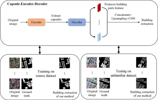
In this study, the encoder is used to capture the parts of the target building, and the building parts are expressed by the vector capsules. The set transformer fuses the building parts’ capsules and obtains the capsule of the target buildings. The decoder reconsiders the correlation from the target buildings to the parts and integrates the correlation information with the parts’ distribution to correct the parts’ distribution in space. We connect the posterior parts’ distribution to obtain the more explainable feature maps. We up-sample these low-resolution feature maps to obtain the segmentation results of the target buildings. In
Figure 5f, most of the target buildings are detected by our method. The performance of our method on the test dataset is best, which proves the feasibility of our method.
For some samples, our method extracts some non-buildings. Most of these areas are gaps between closely spaced groups of buildings. These areas have a small proportion of all pixels. Therefore, these non-buildings do not seriously affect the experimental results. This phenomenon occurs because our method’s ability to segment edges is not strong enough. Our goal is to improve generalization, and we should focus on detecting the main features of the building as much as possible. If the model pays too much attention to edge details, the model will get stuck in the distribution of the source domain, making it difficult to generalize to other domains.
In this paper, three slice images are randomly selected, and the segmentation results are shown in
Figure 6. The first column is the three original images, and the second column is the ground truth. Each of the remaining columns is the building extraction result of a method.
In addition, we record the number of iterations required for each model to converge. Deeplab-v3 and PSPNet have good performance on the test dataset, but the two models are more complicated and require long-term training to achieve convergence. FCN-8s, SegNet, and UNet have a simple structure, but they cannot effectively perceive the characteristics of the target object. Although the three models can converge under short-term training, the performance is not the best. For the attention mechanism of RFA-UNet and the deformable convolution of SegNet+DeformableConv, they need to learn repeatedly to achieve good results. In our method, capsules can effectively perceive the characteristics of the target object, help the model achieve convergence after short-term training, and achieve good performance on the validation dataset. As can be seen from
Table 3, the capsule-based methods all share the same characteristic: they can reach a convergence state with fewer iterations. However, the structure of stacked capsules in CapFPN and HR-CapsNet can realize the role of layer-by-layer abstract features, but it also increases the complexity of the learning process. Our method uses a set transformer to abstract low-level capsules to high-level capsules, reducing the complexity in computation. Therefore, for capsule-based methods, our method can converge faster in training.
3.4. Explainability
Using sliced small-scale remote sensing images, the posterior building part distributions obtained by our method are up-sampled by bilinear interpolation and superimposed on the original image and visualized, as shown in
Figure 7.
Figure 7a–e denote the probability distribution of the existence of each building part in space. The color represents the probability of the existence of the building part. The brighter the color of a region, the greater the activation degree of the building part in that region, that is, the more likely the building part exists. The parts of the target building can be clearly observed in
Figure 7b–d.
Figure 7b reflects that in the second channel, the parts of the target building near the edge and center are more easily detected.
Figure 7c reflects that in the third channel, the edge parts of the target building are more easily detected. Similarly,
Figure 7d corresponds to the detection of the central parts of the target building.
Figure 7g denotes the feature distribution of CNN-based methods, the first row, the second row, and the third row correspond to FCN, SegNet, and UNet in turn. We randomly select three channels from the feature maps output by the convolutional network for visualization, and we can find that these feature distributions are not explainable.
In
Figure 7a,e, the results show that the target object is detected as a whole, which can be considered a larger-scale building part detection result. A further comparison of
Figure 7a,e shows that
Figure 7a is not only activated in the area of the target building but also activated in some local areas of the river, and this result appears reasonable. The target we detect includes buildings along the river shoreline. Therefore, the river can also be broadly considered a part of such buildings. The above results prove the rationality of our method in remote sensing images feature detection.
3.5. Generalization
To verify the generalization performance of our method, we directly apply CNN-based and capsule-based methods to an unfamiliar dataset for inferencing. The performances of these methods are shown in
Table 4. In addition, we randomly sample slice images from this unfamiliar dataset and visualize the building extraction results of these methods, as shown in
Figure 8.
The performance of the CNN-based models on the unfamiliar dataset significantly decreases. For the unfamiliar dataset, the information distribution in images varies greatly, which makes it difficult for convolutional network templates to correctly detect parts of the target object. For
Figure 8c–f, the segmentation results of the mainstream convolutional network models for target buildings are poor. Especially, FCN-8s can hardly detect the existence of buildings.
For Deeplab-v3, multiscale atrous convolution helps the model to obtain more context information. Therefore, Deeplab-v3 can better perceive the target object. The attention mechanism helps RFA-UNet capture the distributions of target objects in remote sensing images, but the performance is not as good as Deeplab-v3. In addition, SegNet+DeformableConv uses deformable convolution, which can adapt to the spatial transformation of target objects’ parts. Therefore, SegNet+DeformableConv performs better than other mainstream convolutional network models. It can be seen from
Table 4 that the
IoU and
PA of SegNet+DeformableConv are relatively small.
Compared to other mainstream convolutional network models, our method can detect the approximate areas of buildings. The above results show that our method has a good generalization ability.
For capsule-based methods, both CapFPN and HR-CapsNet show a significant drop in performance. Although CapFPN and HR-CapsNet both introduce capsule models, both methods only use capsules to store features. Although CapFPN and HR-CapsNet increase the descriptive information of features, these features are not explainable. When we use these methods to reason on unfamiliar datasets, the different statistical distributions cause the process of feature abstraction to deviate from the explainable route; in other words, the final features extracted are completely wrong. Our approach adds out explainability constraints to the capsule model, which allows the model to infer features that are consistent with human visual behavior. Therefore, our method can achieve better generalization.
Furthermore, when we set up a larger number of building parts, our method can better perceive the potential feature information of the target object. Since the capsule can also perceive the spatial relationship of the parts, when we obtain more part features, our method can effectively combine the part features and their spatial relationship to inference about the target object. It can be seen from
Table 4 that when we set the number of parts to 6, the the
IoU and
PA will be further reduced.
Finally, we tested the testing speed of different methods, and the efficiency comparison of different methods is shown in
Figure 9. The results show that our method can achieve good generalization performance with less testing time. The smaller the network size, the faster the testing speed, but the corresponding generalization performance will be reduced.
3.6. Further Experimental Support
To further confirm the generalization of our method, we report the results on the WHU dataset. We experiment with two settings separately. We train methods on the Yellow River training set and test on the WHU test set. In addition, we train methods on the WHU training set, test on the WHU test set, and test on the Yellow River test set.
For the first setting, we treat the WHU dataset as an unfamiliar dataset. We apply three CNN-based methods, two capsule-based methods, and our method to WHU for inferencing. The test performance of various methods is shown in
Table 5. In addition, we randomly sample slice images from the WHU dataset and visualize the building extraction results of these methods, as shown in
Figure 10.
For the second setting, we take the WHU dataset as the source domain. We train one CNN-based method (SegNet+DeConv), two capsule-based methods, and our method on the WHU dataset. We apply these methods to the WHU dataset for inferencing. The test performance of various methods is shown in
Table 6. In addition, we randomly sample slice images from the WHU dataset and visualize the building extraction results of these methods, as shown in
Figure 11.
For generalization of the second setting, we apply these methods to the Yellow River dataset for inferencing. The test performance of various methods is shown in
Table 6. In addition, we randomly sample slice images from the Yellow River dataset and visualize the building extraction results of these methods, as shown in
Figure 12. In our work, extensive experiments show that our method has good generalization.


 ,
, 


