Article

Radar Signal Intrapulse Modulation Recognition Based on a Denoising-Guided Disentangled Network

1
School of Mechanical Engineering and Electronic Information, China University of Geosciences, Wuhan 430074, China
2
School of Information and Electronics, Beijing Institute of Technology, Beijing 100081, China
3
School of Electronic and Communication, Huazhong Universtiy of Science and Technology, Wuhan 430074, China
4
Intelligent Technology Co., Ltd., Chinese Construction Third Engineering Bureau, Wuhan 430074, China
*
Author to whom correspondence should be addressed.
Remote Sens. 2022, 14(5), 1252; https://doi.org/10.3390/rs14051252
Submission received: 19 January 2022 / Revised: 22 February 2022 / Accepted: 1 March 2022 / Published: 4 March 2022
(This article belongs to the Special Issue Radar Techniques for Structures Characterization and Monitoring)

Abstract

:
Accurate recognition of radar modulation mode helps to better estimate radar echo parameters, thereby occupying an advantageous position in the radar electronic warfare (EW). However, under low signal-to-noise ratio environments, recent deep-learning-based radar signal recognition methods often perform poorly due to the unsuitable denoising preprocess. In this paper, a denoising-guided disentangled network based on an inception structure is proposed to simultaneously complete the denoising and recognition of radar signals in an end-to-end manner. The pure radar signal representation (PSR) is disentangled from the noise signal representation (NSR) through a feature disentangler and used to learn a radar signal modulation recognizer under low-SNR environments. Signal noise mutual information loss is proposed to enlarge the gap between the PSR and the NSR. Experimental results demonstrate that our method can obtain a recognition accuracy of 98.75% in the −8 dB SNR and 89.25% in the −10 dB environment of 12 modulation formats.

1. Introduction

Accurate identification of the radar signal intrapulse modulation helps to estimate the function of the radar transmitter and improve the accuracy of radar signal parameter estimation, which is critical in electronic intelligence systems, modern electronic support measure systems, and the radar early warning receiver [1,2,3,4,5]. Nevertheless, the currently widely used pulse compression technique greatly reduces the power spectral density of the radar signal, although it improves the range resolution of the pulse radar. Therefore, under the normal radar operating environments, the signal-to-noise ratio (SNR) of received radar signal is always significantly reduced, thereby seriously affecting the recognition accuracy of radar signal modulation type [6,7]. How to accurately identify the modulation type of radar signals in a low-SNR environment is still an urgent problem to be solved [6].
Traditional intrapulse modulation recognition (IPMR) methods consist of feature extraction and classifier [8]. The accuracy of classic recognition techniques in low-SNR environments is mainly based on feature extraction algorithms, such as high-order cumulants (HOCs), cyclostationary spectrum, instantaneous frequency features, wavelet transformation features, and Wigner Ville distribution (WVD) features [9,10]. Artificial feature extraction is an extremely skillful task that requires researchers with extensive experience. These approaches are difficult to generalize when recognizing new modulation formats. Recently, the works in [4,6,10,11] have proposed to automatically learn discriminative feature representation based on deep convolutional neural networks (DCNNs) to identify radar signal modulation format. However, heavy noise negatively affects the feature learning process of the DCNN when the SNR is low, resulting in the failure to guarantee the high performance of IPMR. Therefore, antinoise embedding is crucial for deep radar IPMR models to automatically extract discriminative feature representation.
Some studies have proposed to denoise radar signals with low SNR before identifying modulation categories through deep convolutional networks [3,12,13,14]. However, these models use denoising as a preprocessing process independent of the modulation recognition step, which is unsuitable for radar signal identification, since the useful signal is inevitably suppressed by noise filters. The residual noise of noncooperative radar signals adversely influences the feature learning of the DCNN when the SNR is below −6 dB [14].
This paper proposes a denoising-guided disentangled network (DGDNet) to recognize intrapulse modulation mode of radar signals at low SNR. We convert the radar modulated signal to time-frequency image (TFI) by using the Cohen class time-frequency distribution (CTFD). Due to the effect of low SNR, TFIs generated directly from CTFD usually contain strong noise. We then use the DGDNet to disentangle the pure radar single representations (PSR) from the noise signal representations (NSR). The signal noise mutual information loss (SNMI) is proposed to broaden the gap between the PSR and NSR. PSR is used to implement radar modulation mode recognition and reduce the effect of noise on classification performance. The DGDNet adopts an end-to-end manner to simultaneously complete denoising and recognition of noisy TFIs, and automatically learn a discriminative radar signal feature expression in a low-SNR environment.
The contributions of this paper are the following:
(1)
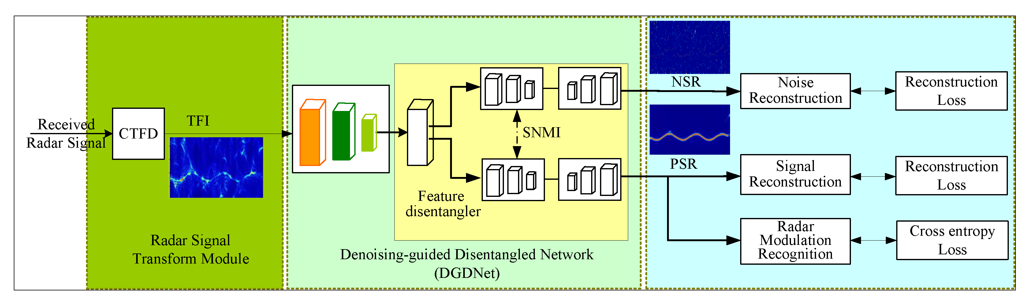
We propose the DGDNet to simultaneously complete the denoising and recognition of noisy TFIs in an end-to-end manner;
(2)
We propose a feature disentangler to extract PSR from NSR and design the SNMI loss to obtain discriminative radar signal feature representation;
(3)
The experimental results demonstrate that the proposed method can obtain a recognition accuracy of 98.75% in the −8 dB SNR and 89.25% in the −10 dB environment of 12 modulation formats.

2. Related Work

Many studies have been conducted on the IPMR of radar signals in recent years. Our work focuses on identifying signal modulations in low-SNR environments.

2.1. Conventional IPMR under Low SNR

Radar intrapulse modulated signals are difficult to detect and identify due to their extremely low peak power, high duty cycle, and other broad spectrum. Many studies on intrapulse feature extraction use signal statistics, such as cumulants (HOC), spectrum, and time–frequency features, as discriminant features to recognize the format of radar signals [15,16]. In [15,16,17], the composite cumulants such as phase jitter, phase offset, and frequency offset are used as extracted features to identify radar intrapulse modulations due to their robustness to noise and model mismatch. Ravi K. and Lunden J. used spectral analysis and instantaneous time-domain to classify digital modulation signals [4,18]. In [11], features extracted from the wavelet transform are used for the identification of multiphase-shift keying and multifrequency-shift keying. In [19,20], an autocorrelation estimator is employed to analyze radar signal features. In [21], radar signal features are analyzed by the Wigner-Hough-Radon transform technique. Chen et al. [22] proposed the feature selection algorithm based on the mutual information between class and feature vector.
Traditional radar modulation recognition methods can correctly recognize the radar modulation formats in normal SNR environments. However, the difficulty of extracting the characteristic parameters within the radar signal pulse also increases as these characteristic parameters become more diverse and fragile. Traditional recognition methods may have problems of low identification accuracy and computational complexity under ultralow-SNR conditions.

2.2. Deep-Learning-Based IPMR in Low-SNR Conditions

Unlike handcrafted feature extraction methods, deep-learning-based models have the capability to automatically capture discriminative feature representations to identify different radar modulation formats.
Artificial neural networks were used as a new method of modulation recognition in [23] for the first time. Most deep learning-based IPMR approaches typically consist of two steps: denoising processing and modulation classification to improve system performance in low-SNR environments. The method proposed in [24] involves designing an eight-layer CNN classifier to identify TFIs, which is preprocessed by a series of 2D Wiener filters, bilinear interpolation and the Otsu method to remove background noise. Qu [14] proposed the convolutional denoising autoencoder (CDAE) to effectively reduce the interference of low SNR on IPMR and improve the classification performance. In [10], a deep autoencoder network for modulation classification was proposed. The network is trained with a non-negative constraint algorithm for constraining negative weights and inferring more meaningful hidden structures. In [25], three network compression and acceleration strategies are proposed, in order to reduce the CNN network’s dependence on computational and memory resources, so that it can be applied to radar platforms with lower computational power and maintain good accuracy. In [26], a neural network applied in postprocessing of radar information is introduced.
Some scholars employ multi-task learning methods for radar modulation pattern recognition. Zhu et al. propose a deep multilabel-based AMC framework to classify the compound radar signals [3]. Wang et al. proposed a multitask learning (MTL)-based method [6] for generalized modulation classification in different noise scenarios.
All the above methods improve the recognition accuracy in low-SNR environments. However, disentangling the pure signal from the noise in deep feature space is a more straightforward solution when the background noise is extremely strong. The denoising and classification tasks can be synchronously completed in an end-to-end way through disentangled learning, and the two tasks can even supervise and promote each other.

2.3. Disentangled Learning

As a method of feature decomposition, disentangled learning aims to correctly reveal a set of independent factors that produce the current observation [23], which has been demonstrated as effective in tasks of image translation and image classification [27]. Interestingly, in [28], Han et al. proposed a disentangled-learning-based network for exploring disentangled general representations in biosignal processing.
In our method, we propose a disentangled framework for not only noise reduction, but also to use disentangled learning to disentangle a low-SNR radar representation into pure PSRs and NSRs. This method has great potential in bridging the gap between radar signal denoising and classification by using DGDNet. It enhances the useful signal by correctly uncovering two independent feature representations in the modulated radar signals.

3. Signal Model and System Overview

3.1. Signal Model

In order to emphasize the disentangling and denoising effects of the DGDNet, we suppose that the modulation parameters of target signal are time-invariant. Additionally, we suppose that only one unknown modulation format signal enters the network at each time. The model of target signal is the following:
r ( t ) = s ( t ) + n ( t ) ,
where r ( t ) is the received signal containing noise, s ( t ) is the useful signal, and n ( t ) is the noise. The modulated signal model of s ( t ) can be represented as
s ( t ) = A · rect ( t / T ) · e j ( a π f c t + ϕ ( t ) + ϕ 0 ) ,
A is the signal amplitude, T is the pulse width, and t indicates the time. f c and ϕ 0 are the carrier frequency and the initial phase, respectively. ϕ ( t ) is the phase function that determines the modulation of the signal. rect ( t ) is a rectangular function. It can be represented as below, and | t | indicates the absolute value of t.
rect ( t ) = 0 , | t | > 1 2 1 2 , | t | = 1 2 1 , | t | < 1 2 .
We focus on the features of the modulated signal ϕ ( t ) . ϕ ( t ) is a quadratic function related to time for a linear frequency modulation (FM) function (LFM), whereas it is a sinusoidal function related to time for a cosine FM function (SFM).
In this paper, n ( t ) is focused on additive Gaussian white noise. We can assume that the variance is σ , the probability density function of n ( t ) can be expressed as
PDF n o i s e ( x ) = 1 2 π · σ · e x 2 2 σ 2 .
SNR is defined as
SNR = 10 · log 10 ( σ s 2 σ n 2 ) ,
where σ s is signal power and σ n corresponds to noise power.

3.2. System Overview

The system can be divided into the following especially vital two parts: radar signal transform module and denoising-guided disentangled network, as we can see in Figure 1.
The radar signal transform module uses the CTFD to transform the radar modulation signal into TFIs. Compared with other widely used time-frequency analysis methods, CTFD has desirable characteristics such as higher resolution, non-negativity, etc. In addition, CTFD can eliminate the cross term of the radar signal through a reasonable design of the kernel function. However, the TFI obtained through the CTFD contains a high noise level under extra low SNR, seriously affecting the recognition accuracy of IPMR.
We propose the DGDNet to strengthen the representation of the modulated radar signal and improve the IPMR recognition accuracy. The pure PSRs and the NSRs are disentangled to reduce the influence of noise signals which are up to identification results. In the meantime, the SNMI loss is proposed to reduce the correlation of NSR and PSR for improving the purity of the PSR. The recognition module is used to obtain the discriminative radar features from the PSR and perform the radar modulation recognition. Reconstruction loss, cross entropy loss, and SNMI loss are jointly used in training the DGDNet to improve the IPMR performance of radar signal under low SNR.

4. Method

4.1. Radar Signal Transform Module

To extract the TFIs from noisy radar signal in low-SNR environments, CTFD is a more suitable time-frequency transformer than others, such as short-time Fourier transform (STFT) and WVD. STFT cuts the signal into small time slices of a certain length. Hence, it is unsuitable for unknown signals. WVD has cross terms that seriously affect the TFIs of nonlinear FM. CTFD can obtain the expected properties, such as higher resolution, being non-negative, and removal of cross terms by smoothing the WVD through time and frequency shifting with a kernel function [28]. The CTFD is defined as
CTFD ( t , ω ) = 1 4 π 2 · AF ( τ , υ ) ϕ ( τ , υ ) · e j υ t j ω τ d υ d τ ,
AF ( τ , υ ) = r ( u + τ 2 ) r * ( u τ 2 ) e j υ u d u ,
where r ( u ) and r * ( u ) are the received signal and its conjugation, respectively. AF ( τ , υ ) is a fuzzy function. τ is the time delay, and υ is the frequency shift. CTFD ( t , ω ) is the time–frequency output. ϕ ( τ , υ ) is the kernel function. The CTFD ( t , w ) is the result of a 2D Fourier transform of the kernel-treated fuzzy functions.
AF ( τ , υ ) can be divided into self-term and interterm. The center of the self-term is located at ( τ , υ ) = ( 0 , 0 ) , and the center position of the interterm directly reflects the shock situation of the signal crossover. The farther the center is from the origin of the plane, the worse the shock.
For modulated signals, such as nonlinear FM signals, especially as PSK and FSK, have cross terms which sorely impact the accuracy of modulation signal recognition. Cross terms of modulated signals are susceptible to noisy signals, resulting in instability. When using the TFIs to identify the signals, we aim to minimize cross terms of the signal while maintaining its hidden characteristics.
The kernel function ϕ ( τ , υ ) is actually a flat 2D low-pass filter that filters the fuzzy function to suppress the cross terms, which is defined as
ϕ ( τ , υ ) = e ( γ τ 2 + ξ ( υ τ ) 2 ) ,
where γ and ξ are used to shape and resize the kernel function. In Figure 2, Figure 2a presents the contour diagram of the kernel function at γ = 0.0005 and ξ = 0. 025, and Figure 2b is the local amplification diagram (with labels) of the kernel function. The kernel function is distributed along the axis and elliptical. This function satisfies most frequency modulation functions, such as SFM, secondary FM signal EQFM, and phase modulation signal PSK, where the fuzzy field interterms are in or around the axis. This condition allows the CTFD of the new nuclear function to have better noise-resistant capability.

4.2. DGDNet

4.2.1. Structure of The Network

The DGDNet is divided into three parts, namely, the global feature extractor (backbone), the feature disentangler, and the modulation mode recognizer. We directly use the Inception_v4 similar backbone as the global feature extractor to pick up the integrated features, including the useful and noise signals in the TFIs. The featured disentangler includes a pure radar feature extractor and a noise feature extractor that are used to obtain the PSR and NSR, respectively. The cosine distance loss between the ideal images and reconstruction images is proposed to supervise the extraction processes of the PSR and NSR. The SNMI loss between the PSR and NSR is proposed to increase the independence between the pure radar feature extraction process and the noise feature extraction process. Discriminative features are automatically extracted by the modulation mode recognizer to perform the radar signal modulation format classification, as shown in Figure 3.

4.2.2. Global Feature Extractor

The global feature extractor is a stem module (Inception_v4 similar backbone) aimed to obtain the deep features of input TFIs. The network roughly consists of nine layers, where three filter cascade layers are found. Correspondingly, the two small branches in front of each concat layer are used to automatically extract discriminative features at different scales. The initial size of the TFIs is 1024 × 1024 . The input TFIs become a tensor with a size of 299 × 299 through image resizing and normalization. The output simultaneously contains the useful information and the noise. Its structure is shown in Figure 4.
The module applies convolution kernels of different sizes to extract image features and achieve feature fusion. The convolution layer ( 1 × 1 convolution) is used to adjust the dimensionality of the feature maps. After the global feature extractor, the network output is a tensor of 35 × 35 × 384 as the input of the pure radar feature extractor and the noise feature extractor.

4.2.3. Feature Disentangler

The output of the global feature extractor is feature maps, including PSR and NSR, and the feature disentangler is devised to progressively disentangle the PSR from the NSR by using the pure radar feature extractor and noise feature extractor.
  • Pure Radar Feature Extractor
    The pure radar feature extractor includes four Inception_A modules, one Reduction_A module, seven Inception_B modules, and one deconvolution module. The Inception module is used to extract the useful signal features hidden in the TFIs. The reduction layer is applied to reduce the image size. The output of the pure radar feature extractor is the PSR, which can be used to classify different modulation formats. The PSR can be used to reconstruct the denoised TFIs through the deconvolution module. This condition motivates us to design the radar signal reconstruction loss as
    L P S R _ c o s ( x r e c n , y i d l ) = 1 N i = q n ( 1 f c o s ( x r e c n , y i d l ) ) ,
    the reconstruction loss L P S R _ c o s is the cosine distance between the ideal denoising image y i d l and pure image x r e c n reconstructed by the deconvolution module. Unfortunately, ideal denoising pictures cannot be obtained in real scenes (confrontation scenes, blind reception scenes). Therefore, we directly use the TFIs transformed from the radar signal under the SNR of 16 dB as the ideal denoising images.
    The details of the modules are shown in Figure 5. Figure 5a presents Inception_A, Figure 5b is Inception_B, Figure 5c is Reduction_A ( k = 192 , l = 224 , m = 256 , n = 384 ), and Figure 5d presents the deconvolution modules (Deconv-modules).
  • Noise Feature Extractor
    Similar to the pure radar feature extractor, the noise signal extractor is based on the Inception structure. It contains one Inception_A module, one Reduction_A module, two Inception_B, and one Deconvolution module. The output of the noise feature extractor is the NSR, which can be used to reconstruct the noise images through the deconvolution module. Similar to the pure radar feature extraction process, the TFIs transformed from the radar signal under SNR of 16 dB can be used as the ideal denoising images. Therefore, the ideal noising images can be calculated as the difference between the input noisy TFIs and the ideal denoising images, as shown in Figure 2. A cosine distance loss L N S R _ c o s is designed to calculate the gap between the noise image and the ideal noising image, which is defined as
    L N S R _ c o s ( p r c n , x i n , y i d l ) = 1 N i = q n ( 1 f c o s ( x i n p r c n , y i d l ) ) ,
    where x i n is the input image, p r c n is the noise picture reconstructed by the noise signal extractor, and y i d l is the ideal pure image.
  • SNMI Loss
    To improve the independence between the PSR and the NSR, we propose the SNMI loss I S N to reduce the correlation between the pure radar feature extraction process and the noise feature extraction process. I S N is defined as
    I S N ( X P S R , X N S R ) = log ( d P p _ n d P p s r d P n s r ) d P p _ n ,
    P p s r = X N S R d P p _ n P n s r = X P S R d P p _ n ,
    where X P S R and X N S R denote the PSR outputted by the pure radar feature extractor and the NSR exported by the noise signal extractor. P p _ n indicates the joint probability distribution between X P S R and X N S R . P p s r and P n s r are the marginal distributions. Minimizing I S N can promote the independence of X P S R and X N S R .

4.2.4. Modulation Mode Recognizer

The modulation mode recognizer contains one Reduction_B module, three Inception_C modules, and one FC layer. The FC layer is followed by the softmax layer to convert the feature representation to the probability values. Followed by the pure radar feature extractor, the recognizer is designed to extract the discriminative feature representation from the PSR to perform the classification of 12 modulation formats.
The Reduction_B and the Inception_C module structures are shown in Figure 6.
The recognizer loss is the cross entropy of the predicted results and the actual modulation mode labels. Cross entropy is defined as
H ( x p r e , y l a b ) = 1 N i = 1 n ( y l a b log x p r e + ( 1 y l a b ) log ( 1 x p r e ) ) ,
where y l a b is the given modulation mode label, and x p r e is the predicted result.
The total loss L t o t a l is defined as
L t o t a l = L P S R _ c o s + L N S R _ c o s + α I S N + H ,
where α is used to normalize I S N for matching with other losses and is set to 0.25 in the experiments.

5. Simulation Result and Analysis

5.1. Dataset Types

Our method identifies 12 types of radar modulation signals, namely, monopulse signals, LFM signal, SFM signal, bilinear FM signal, multiple linear FM, EQFM, binary PSK, binary frequency key-control (2FSK), quad frequency key-control (4FSK), polyphase coded signal (Frank), and composite modulation (LFM-BPSK, 2FSK-BPSK). The corresponding TFIs are shown in Figure 7. The normalized frequency is used, and the number of sampling points is 1000. Figure 7a–l show the TFI of 12 types of radar modulation signals respectively. Figure 7a–e,l have much better time–frequency characteristics. Such time-frequency images are used as datasets for network training.

5.2. Construction of Datasets

Due to the secrecy of radar signals, especially for military radars, it is difficult to obtain real datasets. Therefore, we use a Matlab simulation platform to generate simulation datasets with a large dynamic parameter range (details are shown in Table 1). We take SNR = 16 as pure signal. The signal length is N = 1024, and the sampling rate is 200 MHz. Considering that −10 dB is a very typical low SNR in a practical application environment, most of the current radar modulation identification methods still cannot significantly improve the radar modulation recognition accuracy in the −10 dB SNR environment, especially when the types of radar modulation signals reach 12. Additionally, 8 dB also represents a relatively high SNR level achievable in practical applications. Therefore, in this paper, the evaluating SNR ranges from −10 dB to 8 dB. For every radar modulation type, the number of training and test datasets is 700 and 100 per 2 dB SNR, respectively. Therefore, 84,000 training and 12,000 test samples are used altogether. Each signal adds Gaussian white noise.

5.3. Baseline Methods

We use six methods as performance baselines to demonstrate the supervision of our approach for the IPMR task.
kNN: This model is a classic machine learning method [29] which is used for data mining classification.
SVM: This model is another machine learning method [30]. It is supervised learning models with associated learning algorithms that analyze data for classification and regression analysis.
ADGOONet: This model is a two-stage IPMR that includes the denoising step and recognition step. ADNet [24], which is a state-of-the-art image denoising network proposed in 2020, is used as the denoising filter. In the recognition step, GoogleNet [23] is used to classify the denoised TFIs generated from ADNet.
ADVGGNet: Similar to ADGOONet, the denoising filter is ADNet, and the modulation recognizer is Vgg16.
ADRESNet: This model is also a two-stage IPMR. ADNet is used as a noise filter, and ResNet50 [27] is applied as a modulation format identifier.
INCEPTIONv4 [28]: This model uses classic CNNs for image recognition. It autonomously learns features that are most conducive to image classification and continuously optimizes itself to achieve modulation format recognition.

5.4. Simulation Result and Analysis

We train our networks with stochastic gradient descent and by utilizing the Pytorch platform with 3080ti GPU. We use a learning rate which is set to 0.01, decayed at the 30th, 50th, and 70th epochs with an exponential rate of 0.1. The total number of epochs is 100. The initial image size of the datasets is 1024 × 1024 . Thus, we first use the three interpolation methods to adjust the image size to 64 × 64 , divide each pixel value of the image by 255, and normalize it between 0 and 1. We add a dropout before the FC layer in the modulation mode recognizer to reduce overfitting.
The three baseline methods are compared in Figure 8 to better illustrate the performance of the DGDNet. Table 2 lists the detailed indicators. We define the Overall Probability of Successful Recognition (OPSR) to describe the recognition accuracy of IPMR. OPSR is the ratio of the model’s correct prediction across all test sets.
OPSR = N T p r e N S t e s t ,
where N T p r e is the number of correct prediction of dataset, N S t e s t is the overall number of test dataset. Above an SNR of −6 dB, the OPSR mostly reaches 100%, especially the DGDNet. Below −6 dB, the OPSR of DGDNet exceeds the three other two-stage IPMR models. The end-to-end strategy is effective.
To demonstrate the effectiveness of the feature disentangler and the SNMI loss, we compared the baseline Inceptionv4 and the DGDNet without SNMI loss in Figure 9. The OPSR is greatly improved under low SNR after adding the feature disentangle. Under the SNR of −10 dB, the OPSR increases by approximately 0.7 percentage points. The OPSR is improved in the SNR of −6 and −8 dB in Table 3 after enlarging the independence of PSR and NSR through the SNMI loss. NSL indicates “No SNMI Loss”. Therefore, the feature disentangler and the SNMI loss are extremely effective for improving the recognition of radar signal modulation format in low-SNR environments.

6. Conclusions

In this paper, a novel network called DGDNet is proposed to recognize intrapulse modulation mode of radar signal. The noisy TFIs under low-SNR environments can be obtained through the CTFD. The DGDNet is used to simultaneously complete the denoising and recognition of noisy TFIs in an end-to-end method. Meanwhile, PSR and NSR can be automatically extracted from the feature disentangler to improve the radar signal modulation identification performance in a low-SNR environment. The experimental results are sufficient to encourage us that the proposed method can obtain a final recognition accuracy of 98.75% in the −8 dB SNR and 89.25% in the −10 dB environment of 12 modulation formats.

Author Contributions

X.Z., J.Z. and D.L. contributed to the design and implementation of the research; T.H., Z.T., Y.C. and J.L. contributed to the analysis, processing, and interpretation of the data; T.L. wrote the article with input from all authors. All authors have read and agreed to the published version of the manuscript.

Funding

National Natural Science Foundation of China under grant No. 61973283.

Institutional Review Board Statement

Not applicable.

Informed Consent Statement

Not applicable.

Data Availability Statement

Not applicable.

Conflicts of Interest

The authors declare no conflict of interest.

References

  1. Zuo, L.; Wang, J.; Sui, J.; Li, N. An Inter-Subband Processing Algorithm for Complex Clutter Suppression in Passive Bistatic Radar. Remote Sens. 2021, 13, 4954. [Google Scholar] [CrossRef]
  2. Xu, J.; Zhang, J.; Sun, W. Recognition of The Typical Distress in Concrete Pavement Based on GPR and 1D-CNN. Remote Sens. 2021, 13, 2375. [Google Scholar] [CrossRef]
  3. Zhu, M.; Li, Y.; Pan, Z.; Yang, J. Automatic Modulation Recognition of Compound Signals Using a Deep Multilabel Classifier: A Case Study with Radar Jamming Signals. Signal Process. 2020, 169, 107393. [Google Scholar] [CrossRef]
  4. Ravi Kishore, T.; Rao, K.D. Automatic Intrapulse Modulation Classification of Advanced LPI Radar Waveforms. IEEE Trans. Aerosp. Electron. Syst. 2017, 53, 901–914. [Google Scholar] [CrossRef]
  5. Sadeghi, M.; Larsson, E.G. Adversarial Attacks on Deep Learning-based Radio Signal Classification. IEEE Wirel. Commun. Lett. 2019, 8, 213–216. [Google Scholar] [CrossRef] [Green Version]
  6. Wang, Y.; Gui, G.; Ohtsuki, T.; Adachi, F. Multi-Task Learning for Generalized Automatic Modulation Classification under Non-Gaussian Noise with Varying SNR Conditions. IEEE Trans. Wirel. Commun. 2021, 20, 3587–3596. [Google Scholar] [CrossRef]
  7. Yu, Z.; Tang, J.; Wang, Z. GCPS: A CNN Performance Evaluation Criterion for Radar Signal Intrapulse Modulation Recognition. IEEE Commun. Lett. 2021, 25, 2290–2294. [Google Scholar] [CrossRef]
  8. Hassan, K.; Dayoub, I.; Hamouda, W.; Nzeza, C.N.; Berbineau, M. Blind Digital Modulation Identification for Spatially Correlated MIMO Systems. IEEE Trans. Wirel. Commun. 2012, 11, 683–693. [Google Scholar] [CrossRef]
  9. Wang, Y.; Gui, J.; Yin, Y.; Wang, J.; Sun, J.; Gui, G.; Adachi, F. Automatic Modulation Classification for MIMO Systems via Deep Learning and Zero-Forcing Equalization. IEEE Trans. Veh. Technol. 2020, 69, 5688–5692. [Google Scholar] [CrossRef]
  10. Ali, A.; Yangyu, F. Automatic Modulation Classification Using Deep Learning Based on Sparse Autoencoders with Nonnegativity Constraints. IEEE Signal Process. Lett. 2017, 24, 1626–1630. [Google Scholar] [CrossRef]
  11. Peng, S.; Jiang, H.; Wang, H.; Alwageed, H.; Zhou, Y.; Sebdani, M.M.; Yao, Y.D. Modulation Classification Based on Signal Constellation Diagrams and Deep Learning. IEEE Trans. Neural Netw. Learn. Syst. 2019, 30, 718–727. [Google Scholar] [CrossRef] [PubMed]
  12. Tian, C.; Xu, Y.; Li, Z.; Zuo, W. Attention-guided CNN for Image Denoising. Neural Netw. 2020, 124, 117–129. [Google Scholar] [CrossRef] [PubMed]
  13. Qu, Z.; Hou, C.; Wang, W. Radar Signal Intra-Pulse Modulation Recognition Based on Convolutional Neural Network and Deep Q-Learning Network. IEEE Access 2020, 8, 49125–49136. [Google Scholar] [CrossRef]
  14. Qu, Z.; Wang, W.; Hou, C. Radar Signal Intra-Pulse Modulation Recognition Based on Convolutional Denoising Autoencoder and Deep Convolutional Neural Network. IEEE Access 2019, 7, 112339–112347. [Google Scholar] [CrossRef]
  15. Azzouz, E.E.; Nandi, A.K. Automatic Identification of Digital Modulation Types. Signal Process. 1995, 47, 55–69. [Google Scholar] [CrossRef]
  16. Zhang, L.; Yang, Z.; Lu, W. Digital Modulation Classification Based on Higher-order Moments and Characteristic Function. In Proceedings of the 2020 IEEE 5th International Conference on Signal and Image Processing (ICSIP), Nanjing, China, 23–25 October 2020. [Google Scholar]
  17. Zaerin, M.; Seyfe, B. Multiuser Modulation Classification Based on Cumulants in Additive White Gaussian Noise Channel. IET Signal Process. 2012, 6, 815–823. [Google Scholar] [CrossRef]
  18. Lunden, J.; Terho, L.; Koivunen, V. Waveform Recognition in Pulse Compression Radar Systems. In Proceedings of the 2005 IEEE Workshop on Machine Learning for Signal Processing, Mystic, CT, USA, 28 September 2005. [Google Scholar]
  19. Warde, D.A.; Torres, S.M. The Autocorrelation Spectral Density for Doppler-Weather-Radar Signal Analysis. IEEE Trans. Geosci. Remote Sens. 2014, 52, 508–518. [Google Scholar] [CrossRef]
  20. Shi, Z.; Wu, H.; Shen, W.; Cheng, S.; Chen, Y. Feature Extraction for Complicated Radar PRI Modulation Modes Based on Auto-correlation Function. In Proceedings of the 2016 IEEE Advanced Information Management, Communicates, Electronic and Automation Control Conference (IMCEC), Xi’an, China, 3–5 October 2016. [Google Scholar]
  21. Gulum, T.O.; Erdogan, A.Y.; Yildirim, T.; Pace, P.E. A Parameter Extraction Technique for FMCW Radar Signals Using Wigner-Hough-Radon Transform. In Proceedings of the 2012 IEEE National Radar Conference, Atlanta, GA, USA, 7–11 May 2012. [Google Scholar]
  22. Chen, Y.; Nijsure, Y.; Yuen, C.; Chew, Y.H.; Ding, Z.; Boussakta, S. Adaptive Distributed MIMO Radar Waveform Optimization Based on Mutual Information. IEEE Trans. Aerosp. Electron. Syst. 2013, 49, 1374–1385. [Google Scholar] [CrossRef]
  23. Wu, A.; Han, Y.; Zhu, L.; Yang, Y. Instance-Invariant Domain Adaptive Object Detection via Progressive Disentanglement. IEEE Trans. Pattern Anal. Mach. Intell. 2021; in press. [Google Scholar]
  24. Qu, Z.; Mao, X.; Deng, Z. Radar Signal Intrapulse Modulation Recognition Based on Convolutional Neural Network. IEEE Access 2018, 6, 43874–43884. [Google Scholar] [CrossRef]
  25. Chen, H.; Zhang, F.; Tang, B.; Yin, Q.; Sun, X. Slim and Efficient Neural Network Design for Resource-Constrained SAR Target Recognition. Remote Sens. 2018, 10, 1618. [Google Scholar] [CrossRef] [Green Version]
  26. Jan, M.; Pietrow, D. Artificial Neural Networks in The Filtration of Radiolocation Information. In Proceedings of the 2020 IEEE 15th International Conference on Advanced Trends in Radioelectronics, Telecommunications and Computer Engineering (TCSET), Lviv-Slavske, Ukraine, 25–29 February 2020. [Google Scholar]
  27. Deng, W.; Zhao, L.; Liao, Q.; Guo, D.; Kuang, G.; Hu, D.; Liu, L. Informative Feature Disentanglement for Unsupervised Domain Adaptation. IEEE Trans. Multimed. 2021; in press. [Google Scholar]
  28. Han, M.; Özdenizci, O.; Wang, Y.; Koike-Akino, T.; Erdoğmuş, D. Disentangled Adversarial Autoencoder for Subject-Invariant Physiological Feature Extraction. IEEE Signal Process. Lett. 2020, 27, 1565–1569. [Google Scholar] [CrossRef] [PubMed]
  29. Cover, T.; Hart, P. Nearest neighbor pattern classification. IEEE Trans. Inf. Theory 1967, 13, 21–27. [Google Scholar] [CrossRef]
  30. Cortes, C.; Vapnik, V. Support-vector network. Mach. Learn. 1995, 20, 273–297. [Google Scholar] [CrossRef]
Figure 1. The overall framework of the system.
Remotesensing 14 01252 g001
Figure 2. CTFD’s kernel function contour diagram. (a) The contour diagram at γ = 0.0005 and ξ = 0.025; (b) Local amplification diagram.
Remotesensing 14 01252 g002
Figure 3. Detailed structure of the network.
Remotesensing 14 01252 g003
Figure 4. Structure of the stem module.
Remotesensing 14 01252 g004
Figure 5. Module details: (a) Inception_A; (b) Inception_B; (c) Reduction_A; (d) Deconv-module.
Remotesensing 14 01252 g005
Figure 6. The module structure: (a) Reduction_B; (b) Inception_C.
Remotesensing 14 01252 g006
Figure 7. TFIs of different modulation modes: (a) LFM; (b) SFM; (c) DLFM; (d) MLFM; (e) MP; (f) BPSK; (g) Frank; (h) 2FSK; (i) 4FSK; (j) LFM-BPSK; (k) 2FSK-BPSK; (l) EQFM.
Remotesensing 14 01252 g007
Figure 8. Comparison with the CDAE-DCNN in [6]. Among them, classical machine learning algorithms such as SVM and kNN have unsatisfactory accuracy, while deep-learning-based methods are more competitive in accuracy regardless of low SNR or high SNR.
Remotesensing 14 01252 g008
Figure 9. Comparison of the DGDNet with different parameters and Inception_v4 [28]. As can be seen in the figure, Inception_v4’s performance below −4 dB is inferior to that of DGDNet proposed by us. Meanwhile, DGDNet performed better with SNMI.
Remotesensing 14 01252 g009
Table 1. Simulation signal parameters [24].
ParametersValues
Modulation type numbers12
Number of sample points1024
Sampling rate200 MHz
Number of training samples200 samples/type/SNR
SNR ∈ [−10:2:8] (dB)
Number of test samples100 samples/type/SNR
SNR ∈ [−10:2:8] (dB)
Training samples/test samples7/1
Parameters of Gaussian white noise N ( 0 , σ n 2 )
σ n 2 = σ s 2 / ( SNR 10 ) 10
Bandwidth of different signals10 MHz: 80 MHz
Phase number of Frank4, 5, 6, 7
Minimum frequency interval of FSK10 MHz
Table 2. Detailed indicators of four methods.
SNR−10−8−6−4−202468
kNN0.31840.33970.40790.43360.46730.56120.57640.58030.60530.6374
SVM0.42970.56540.60730.69630.70740.83520.85640.86550.89230.8991
DGDNet0.89250.98750.99911111111
ADGOONet0.78040.94810.9961111111
ADVGGNet0.76520.93920.9961111111
ADRESNet0.76650.93870.99330.99960.999610.99960.999610.9996
Table 3. Detailed indicators of three approaches.
SNR−10−8−6−4−202468
Inception_v40.82670.9550.9950.999210.99921110.9992
DGDNet(NSL)0.8950.980.99830.9992111111
DGDNet0.89250.98750.99911111111
Publisher’s Note: MDPI stays neutral with regard to jurisdictional claims in published maps and institutional affiliations.

